
Energy and Information Fluxes at Upper Ocean Density Fronts

1
Department of Mechanical Engineering, Faculty of Engineering, University of Concepción, Concepción 4070409, Chile
2
Department of Geophysics, Faculty of Physical and Mathematical Sciences, University of Concepción, Concepción 4070386, Chile
*
Author to whom correspondence should be addressed.
†
Interdisciplinary Center for the Aquaculture Research (INCAR), Concepción 4070007, Chile.
Fluids 2023, 8(1), 17; https://doi.org/10.3390/fluids8010017
Submission received: 16 November 2022
/
Revised: 15 December 2022
/
Accepted: 22 December 2022
/
Published: 2 January 2023
(This article belongs to the Special Issue Turbulent Flow, 2nd Edition)
Abstract
:We present large eddy simulations of a midlatitude open ocean front using a modified state-of-the-art computational fluid dynamics code. We investigate the energy and information fluxes at the submesoscale/small-scale range in the absence of any atmospheric forcing. We find submesoscale conditions (∼1, ∼1) near the surface within baroclinic structures, related to partially imbalanced frontogenetic activity. Near the surface, the simulations show a significant scale coupling on scales larger than ∼ (m). This is manifested as a strong direct energy cascade and intense mutual communication between scales, where the latter is evaluated using an estimator based on Mutual Information Theory. At scales smaller than ∼ (m), the results show near-zero energy flux; however, at this scale range, the estimator of mutual communication still shows values corresponding with a significant level of communication between them. This fact motivates investigation into the nature of the self-organized turbulent motion at this scale range with weak energetic coupling but where communication between scales is still significant and to inquire into the existence of synchronization or functional relationships between scales, with emphasis on the eventual underlying nonlocal processes.
1. Introduction
In the past two decades, numerical predictions and observations have revealed a richness of turbulent submesocale processes in the upper ocean. Within these interesting turbulent upper ocean processes, there has been special interest in the study of density fronts to strengthen the understanding of the processes that catalyze smaller-scale motion in order to parameterize them. Such processes include frontogenesis [1,2], frontal instabilities, and the breakdown of balanced flow [3,4,5,6] and their role in promoting the collapse of baroclinical waves and the generation of submesoscale eddies, the mixed-layer restratification [7], the flattening of the spectra in the submesoscale range [8], the development of the direct energy cascade [9,10], and the development of high vertical velocities [4,6,11], as well as their important implications for primary productivity and climate [11].
Density fronts are ubiquitous in the ocean. They tilt the isopycnals and, hence, restratify the mixed layer, causing a secondary circulation with high vertical velocities [12,13]. The main departure from balance occurs in the vicinity of fronts, where the flow is strongly affected by the secondary circulation, which involves frontogenesis [8] and which can also be promoted by alongfront winds [14]. Fronts have also been identified as regions with high energy dissipation, high turbulent mixing [2] and where the direct energy cascade can take place given the high vertical shear due to frontogenesis [15].
Recent research on complex systems and turbulence has investigated the characteristics of communication [16,17,18] and information flows [19,20] between the scales of motion, giving an alternative standpoint that allows for building a more complex picture of the phenomenon of turbulence by complementing the current purely dynamic view based on classical mechanics with features from information theory.
The aim of the present manuscript is to investigate the energy and information fluxes at the submesoscale/small-scale range in a midlatitude upper ocean front using results from a highly resolved LES model allowing simulation of the submesoscale–small scale range directly in order to analyze the characteristics of information flow in the context of current knowledge of this widely studied turbulent system. A state-of-the-art computational fluid dynamics (CFD) code is used to adapt the large eddy simulation (LES) model for geophysical flows. This configuration and detailed descriptions of hydrodynamics and turbulence modeling were previously reported by [21].
2. Computational Model
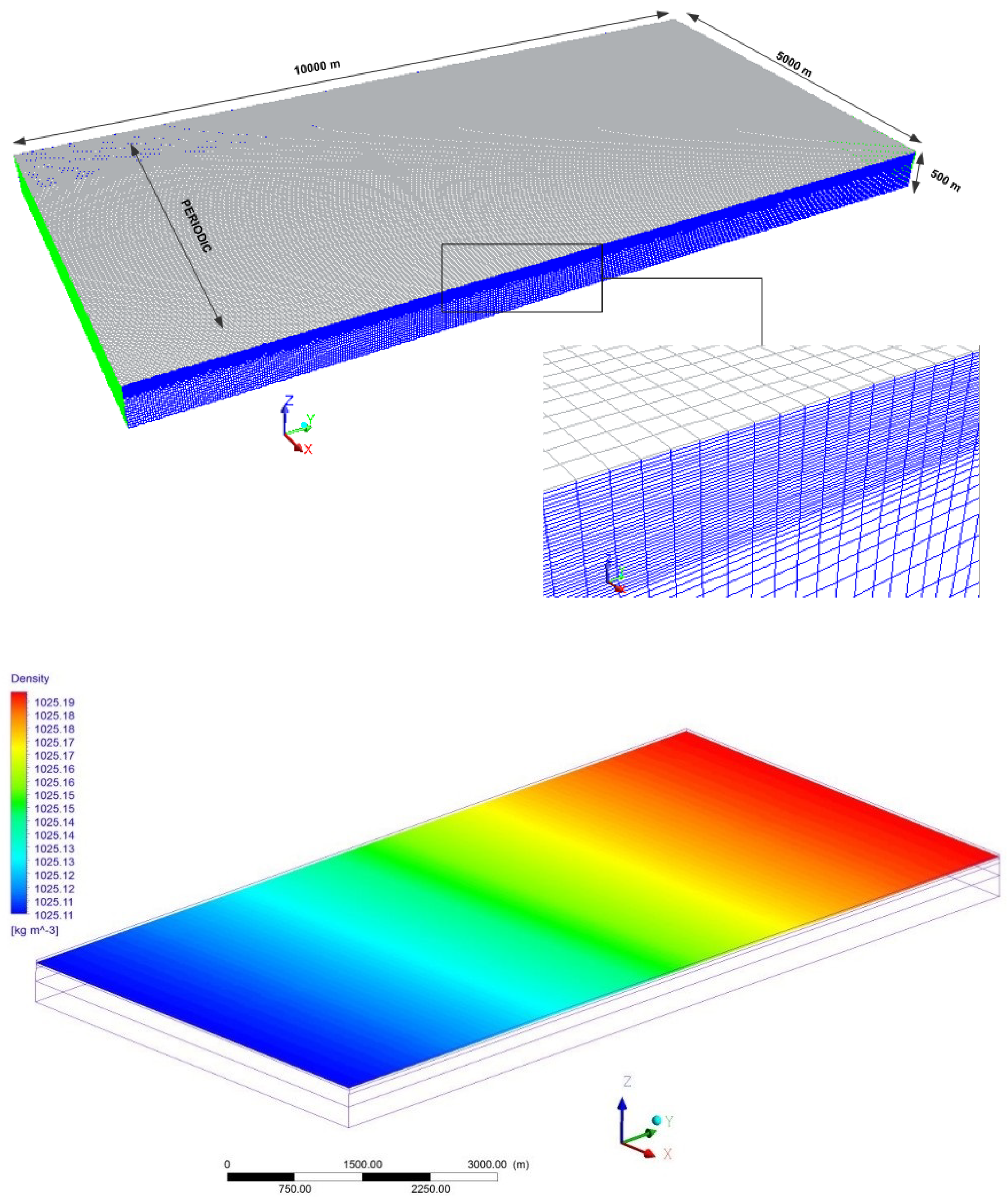
Simulations were performed using a periodic nonhydrostatic LES model [21]. The state-of-the-art CFD code ANSYS-FLUENT was modified to include the Earth’s rotation and water column stratification in order to describe the geophysical fluid flows. For the calculation of subgrid stresses, the well-known Smagorinsky model [22] was modified to employ a nonisotropic computational grid introducing the correction proposed by [23] into the calculation of the mixing length. This modification allowed us to use nonisotropic grids when the usage of an isotropic grid was prohibitive due to limitations regarding the computational capacity. The size of the model domain was 10 km in the crossfront direction, 5 km in the alongfront direction, and 500 m in depth (Figure 1 top). The domain was discretized with cells, with a hexahedral grid of 24 m for the horizontal resolution, a constant 3 m vertical resolution within the first 50 m of depth, a stretched vertical resolution between the depths of 50 m (dz = 3 m) and 250 m (dz = 24 m), and a constant 24 m vertical resolution between the depths of 50 m and 500 m. The model time step was 120 s.
The domain alongfront direction was periodic, and the crossfront direction as well as the top and bottom were taken to be stress-free boundaries. We used Second Order Discretization Schemes and the Least Squares Cell-Based Method to calculate the gradients. For the pressure–velocity coupling the SIMPLE (semi-implicit method for pressure-linked equations) algorithm was adopted.
The model was initialized with a 50 m deep mixed layer and stable stratification between 50 m and 500 m. Within the first 50 m, the density distribution in the crossfront direction was given by
with kg/m, where y represented the horizontal coordinate in the acrossfront direction, as shown in Figure 1 bottom. Below the mixed layer, the horizontal density gradient extended up to a depth of 250 m. In this zone,
where z was the vertical coordinate. The velocity field was initialized with a baroclinic jet in thermal wind balance
where u was the velocity in the alongfront direction and the pressure p was estimated from the hydrostatic balance
with g as the acceleration due to gravity. The model was set up using a midlatitude Coriolis parameter s. This simulation did not consider any atmospheric forcing (winds, heating, cooling, etc.).
3. Energy Transfer, Hydrodynamics, and Information Processes
3.1. Energy Transfer and Hydrodynamics Processes
A spectral representation of the kinetic energy balance is presented below (Equation (5)), where the local variation of kinetic energy in the wave number space was estimated by the sum of the right-side terms, which described, from left to right, the advection of kinetic energy, pressure work, the buoyancy term, and dissipation.
Here, u is the velocity vector, p is the pressure, w denotes the vertical velocity component, b is the buoyancy, and D is the dissipative term. The operators and denote the Fourier transform and conjugate, respectively. Through the integration of the advective term of Equation (5) over an appropriate k shell to , it is possible to estimate the spectral kinetic energy flux and to express the kinetic energy cascade explicitly as
where is the maximum wavelength allowed by the domain dimensions.
The intensity of the frontogenesis can be addressed by the calculation of the frontogenesis parameter , which is a measure of the modification of the horizontal buoyancy gradient magnitude due to the straining by the geostrophic flow [6,8,13], where
is the horizontal density gradient, and the Q vector is given by
Here, are the horizontal velocity components in the directions, and is the density.
We were interested in determining whether the processes promoting the direct energy cascade were related to a balanced or unbalanced dynamics. The balance of pressure, Coriolis, and centrifugal forces is expressed as in [26]:
The degree of imbalance is assessed by the normalized error in the gradient wind balance:
3.2. Information-Related Processes
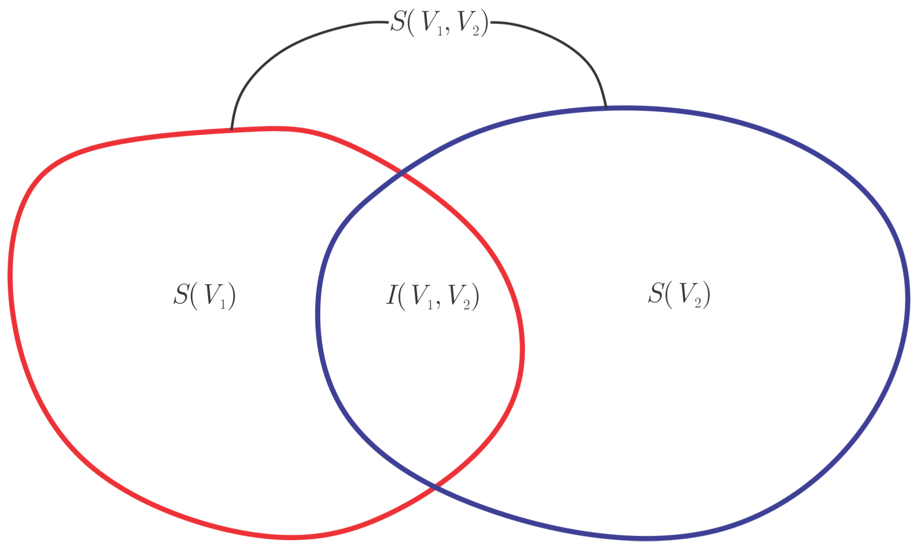
Shannon’s entropy is a quantity associated with the information content in a complex system, interpreted in a statistical sense. If the probability of an event is 1, then it does not give us information; we know that the event will always happen. The same thing happens when the probability is 0; we do not obtain information about those events since they never happen. Due to these properties, entropy is a concave functional in the probability density function; it reaches a maximum between probability 0 and 1. Therefore, entropy can be interpreted as the information content or predictability of a system; the higher the entropy, the less predictable the system. On the other hand, the mutual information measures the amount of information shared between two systems; this can be interpreted as the information contained in the correlations or interactions of two systems. If the systems are independent, then the mutual information is zero, and their joint probability can be broken down as a product. Note how the mutual information and entropy complement each other. If the mutual information between two systems is zero, then the (joint) entropy of both is simply the sum of their individual entropy, while when they interact, there is a contribution to the entropy that is only due to the interactions.
If we have a system with a (marginal) probability density and another with a density , their joint density will be . The entropy of a single system is defined by
while their mutual information is
The relationship between both quantities can be summarized in a diagram shown in Figure 2.
One of the problems we face in calculating these quantities is that they depend on density functions; this complicates things, especially when they have long probability tails, as in the case of turbulence. Due to this, the theory proposes the use of estimators; one of the best known and applied is the ’nearest neighbors’ type, which we used in this study to calculate the entropy and mutual information.
In this work, we used the Kozachenko–Leonenko estimator for the entropy [28],
In the case of mutual information, we used the Kraskov–Stögbauer–Grassberger estimator (KSG) [29]
In both equations, represents the digamma function, N is the number of data, is a distance dependent on the value of k, are the number of points that are less than apart, and represents the average. In both estimators, we have a free parameter k, which is the number of nearest neighbors to consider. This was used to determine the value of and in the KSG algorithm and in the KL algorithm. In this study, was set for the estimation of both quantities (the value recommended in previous studies for turbulent systems [17]). The algorithm used for the mutual information was the one first proposed by [30], which partitions the space into a square grid. Finally, we mention that the distance selected to apply the estimators was the Euclidean distance.
4. Simulation
Using the model described above, we simulated the time evolution of the density front for 20 days. The front began meandering and developing instabilities within the mixed layer two days after initialization. These instabilities became increasingly large in amplitude, resulting in its collapse and the subsequent emergence of coherent structures around the fourth day. Near the seventh day, the turbulence was fully developed. We show the results from nine days after the model’s initialization.
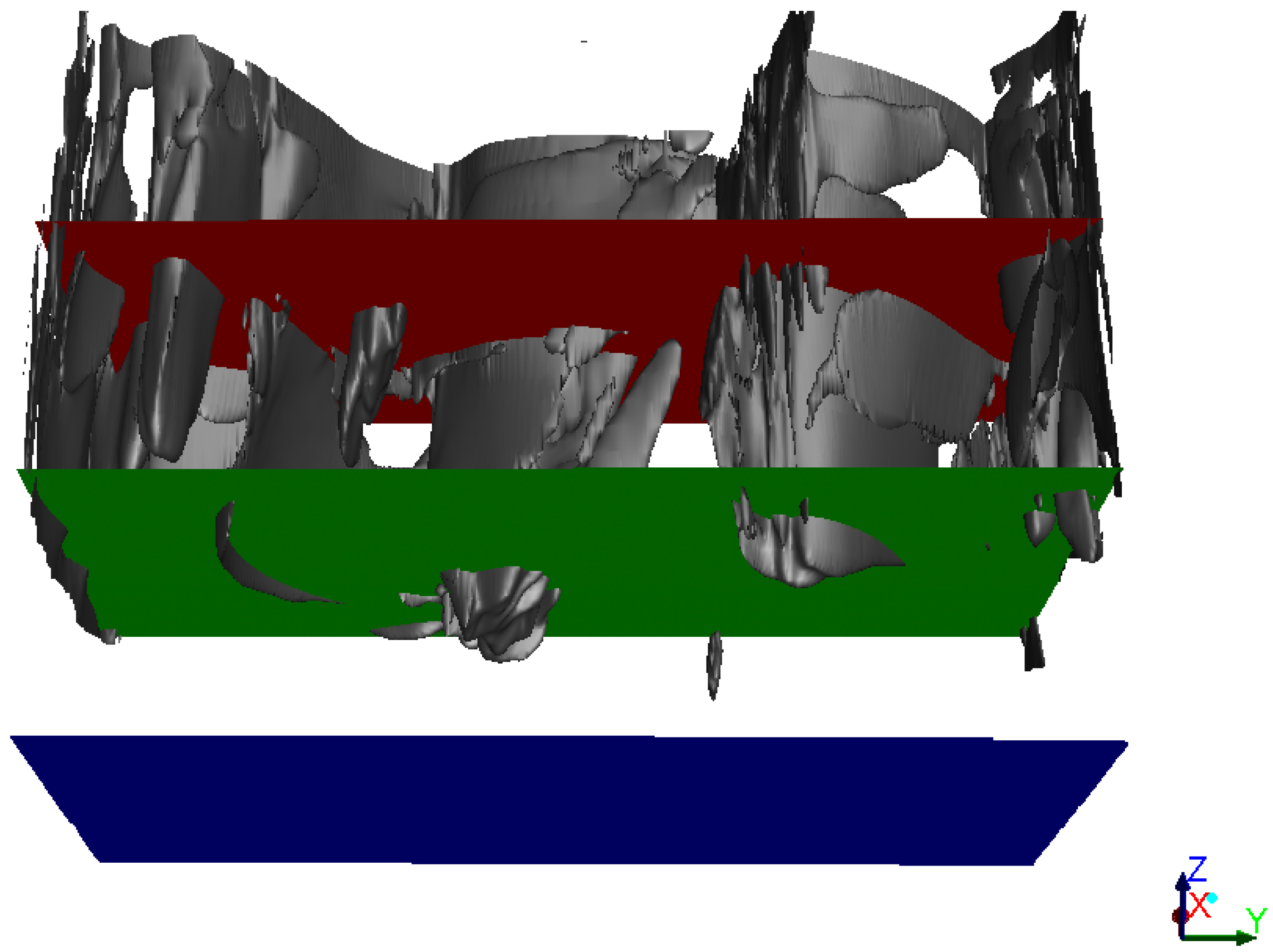
The results showed a strongly unstable shear flow within the first 50 m of depth. In Figure 3, we plot an isosurface of , and the plane colored green is located at a depth of 50 m. This 3D representation of the submesoscale structures has been overlaid in all snapshots considered in the present analysis; thus, one can directly observe the spatial correlation between the variable under consideration and the submesoscale structure.
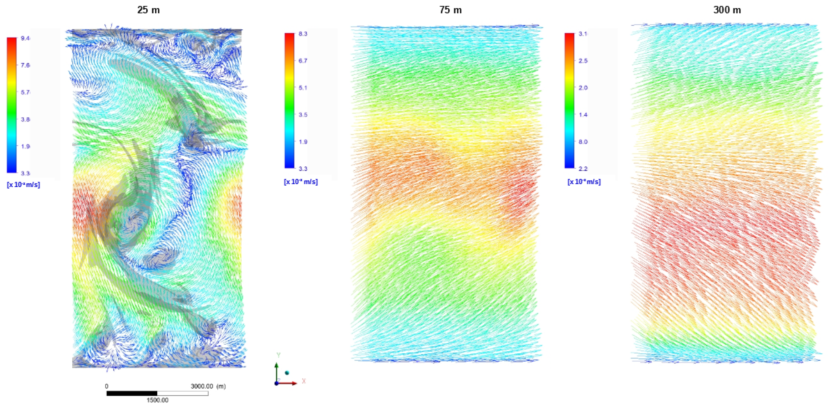
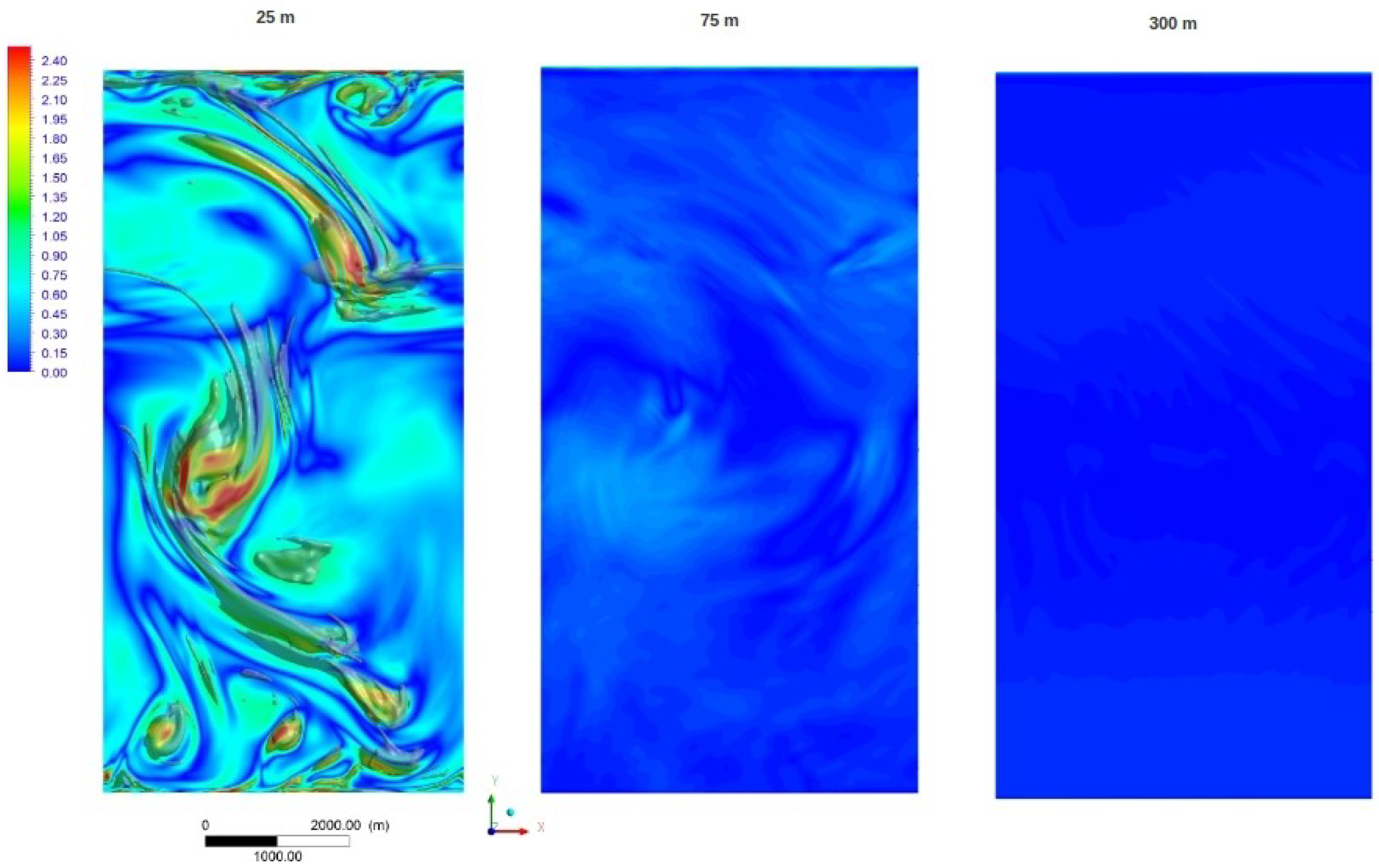
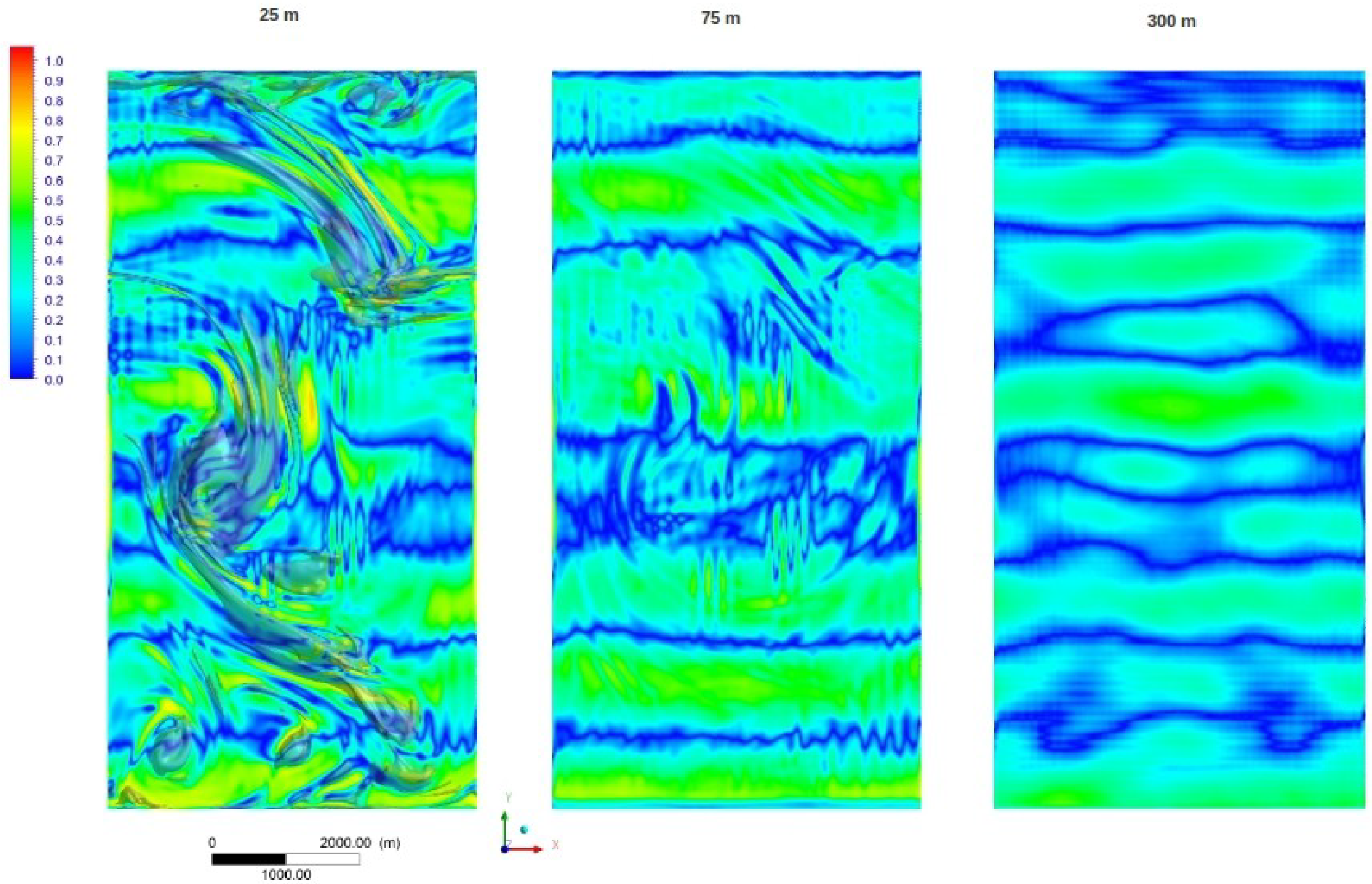
Figure 4 shows the velocity field. In contrast to the flow characteristics found within the mixed layer, below 50 m in depth, the flow was marginally unstable, thereby indicating that even in the unforced case considered here, ocean fronts promote turbulent mixing in the upper ocean, which is consistent with the observations [14]. The Rossby number distribution was estimated from the vertical relative vorticity through . Regions of ∼1 were found only in the first 50 m of depth within the mixed layer. Inside the submesoscale structures, the Rossby number took even higher values as shown in the left panel of Figure 5.
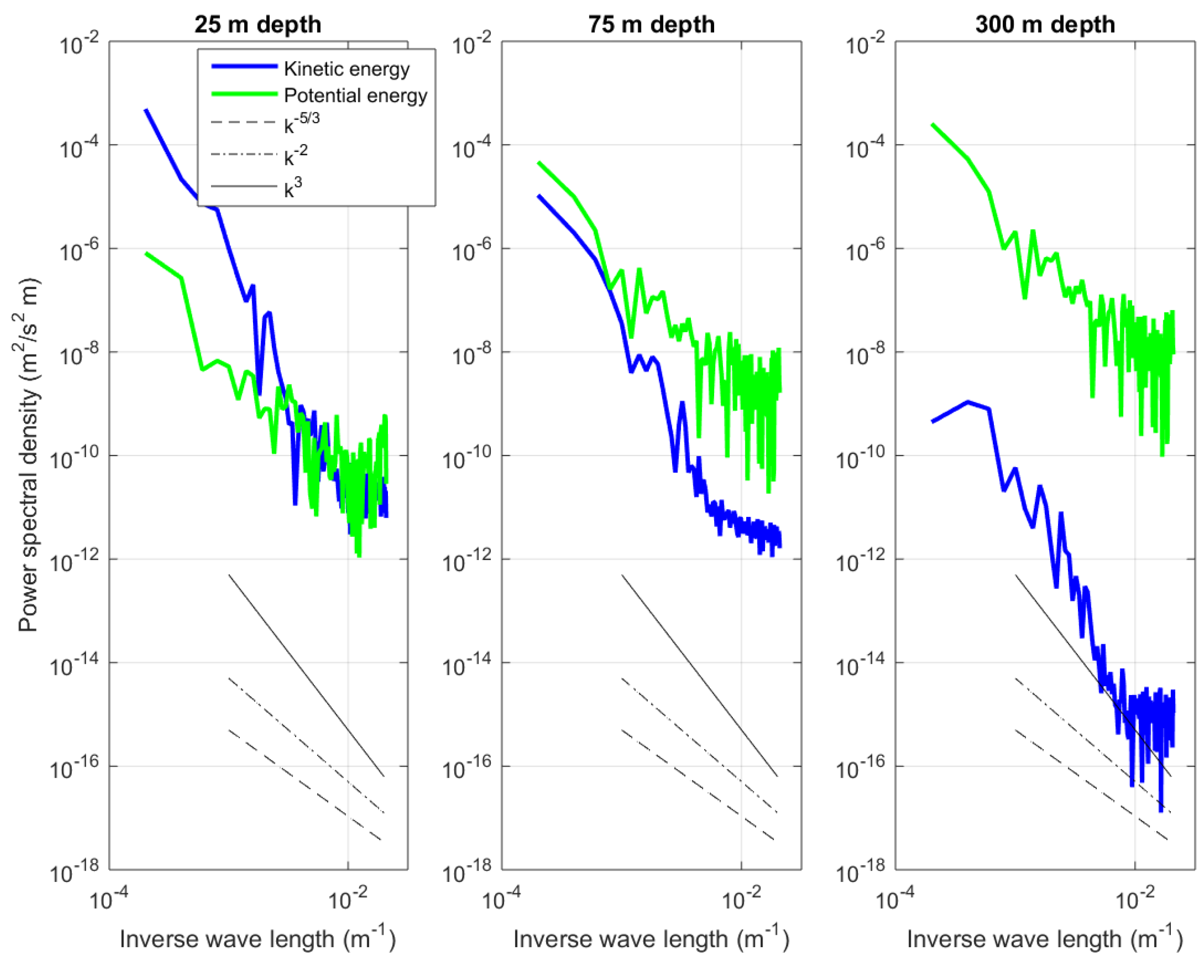
At 75 m deep, there were only few regions where the Rossby number reached a maximum value of ∼0.4, and ∼0.1 was found in the deeper waters at 300 m (right panel of Figure 5). Through the inspection of the kinetic energy spectra, one can indirectly infer some characteristics of the kinetic energy cascade of turbulent flows. The interior quasi-geostrophic theory [30] predicted for the balanced mesoscale flow a kinetic energy spectrum slope of −3, indicating an inverse energy cascade. The submesoscale dynamics have been shown to flatten the spectral kinetic energy distribution to a −2 slope [4], and although the surface quasi-geostrophic theory [31] predicted the same spectrum shape, this theory, as a model for submesoscale dynamics, poorly described the direct kinetic energy cascade present in simulations including nongeostrophic processes [32]. In this case, the surface quasigeostrophic theory, including nongestrophic processes predicted a spectrum with a slope of −5/3 [33].
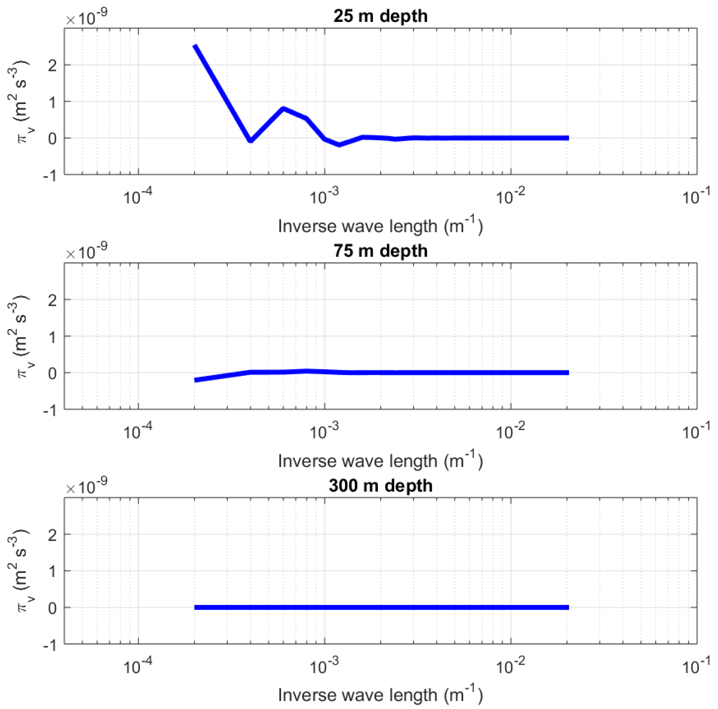
We computed the 1D kinetic and potential energy spectra, using the transects of the horizontal velocity and density variation at different depths, as shown in Figure 6. The turbulent structures were found to be more energetic within the top 50 m of the mixed layer. In this region, the spectrum was flatter than the spectrum computed at 75 m deep in the range of length scale between 0 m and 125 m, which was in agreement with the previous work [4,11]. The calculations of the spectral kinetic energy flux plotted in Figure 7 indicated that in the near ocean surface region, at 25 m deep, a strong direct kinetic energy flux occurred for the horizontal scales larger than 1 km. At the same depth, for scales somewhat smaller than 1 km, the results showed an inverse kinetic energy flux of similar magnitude to the inverse kinetic energy flux that took place at 75 m deep for horizontal scales larger than 2.5 km. In deeper waters, the spectral kinetic energy flux was weak.
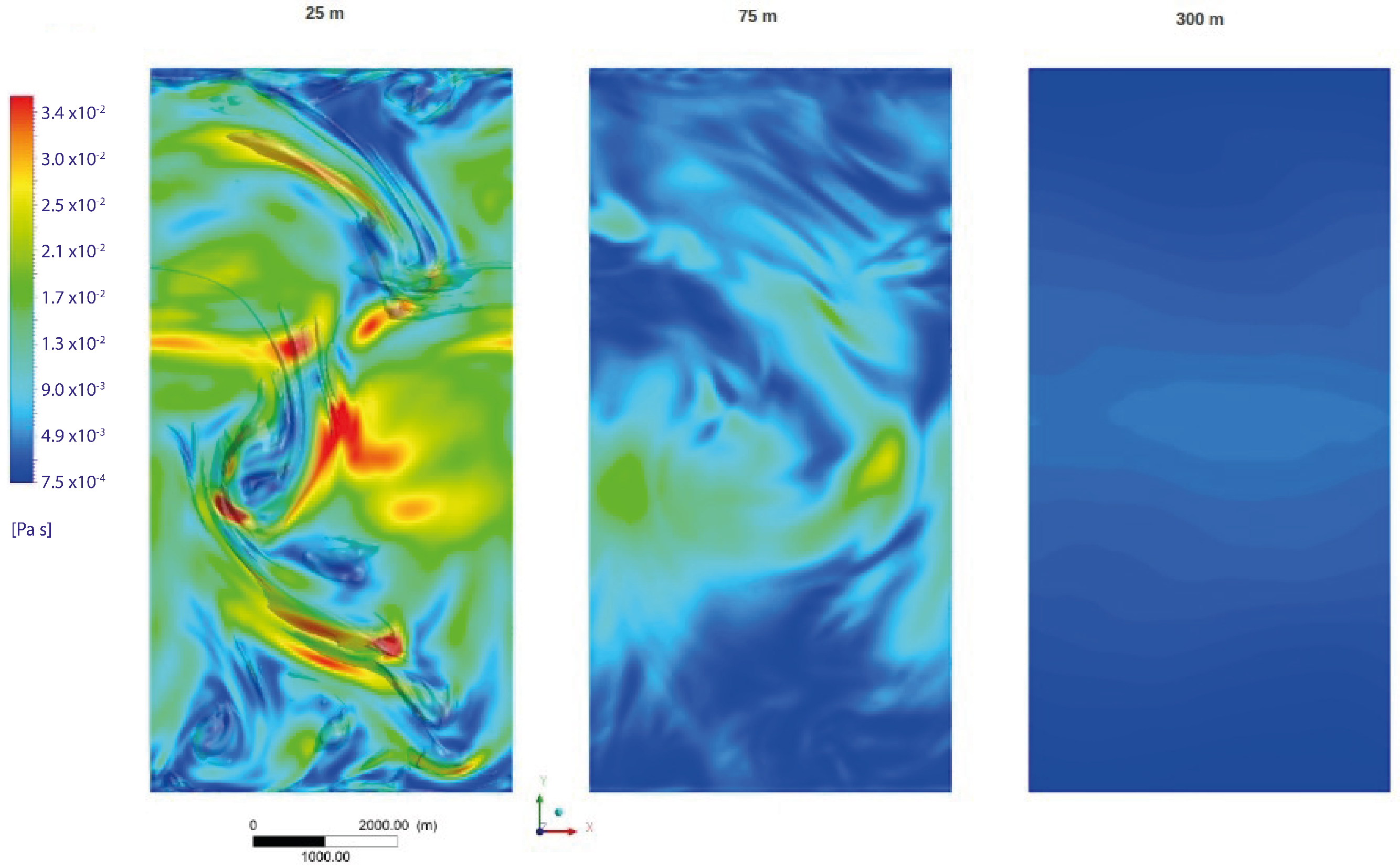
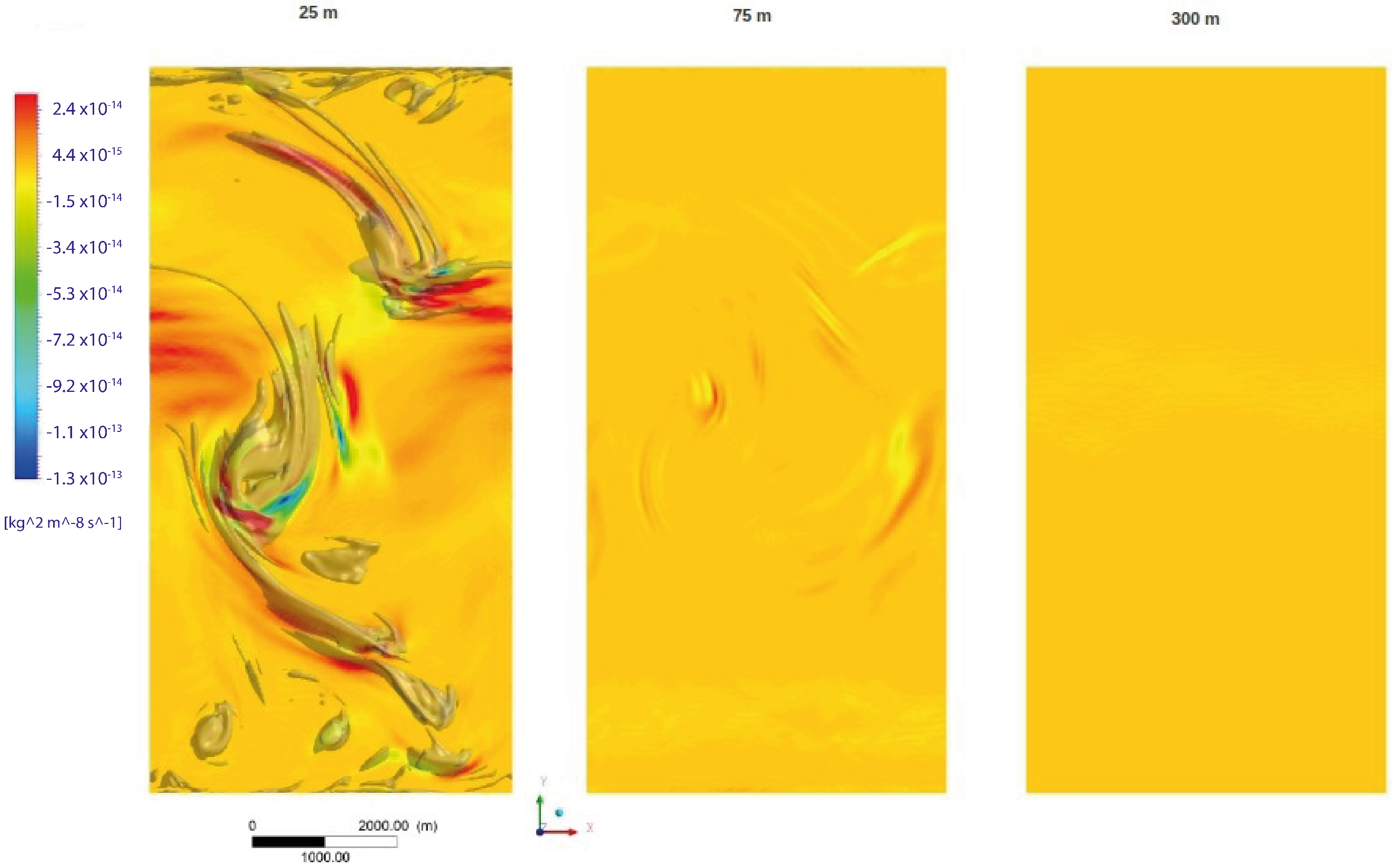
In the LES models, the subgrid momentum diffusion is also a measure of the turbulent kinetic energy dissipation at the subgrid scale [34]. Figure 8 shows the subgrid momentum diffusion at the depths of 25 m, 75 m, and 300 m. The near surface results showed large zones of high subgrid momentum diffusion, while at higher depths, these zones became smaller in extension and intensity. These findings were not surprising and were in the same direction as the predictions of the direct kinetic energy flux; in the absence of atmospheric forcing and due to the frontal processes, the upper ocean is subject to direct kinetic energy flux and high subgrid momentum diffusion.
The difference from the gradient wind balance was computed and plotted in Figure 9. In agreement with [8], the unbalanced pattern was found to be affected by the frontogenetic activity (Figure 10). The processes within the mixed layer were found to be partially imbalanced, where only a few small regions adjacent to the submesoscale structures reached values near . However, apart from these limited small regions, reached values between and ; hence, it was not possible to assess the predominance of the balanced or unbalanced processes in the promotion of the direct kinetic energy flux.
Given turbulence is a scaling phenomenon, we studied the entropy distribution in Fourier space. We used the same 1D velocity transects employed to calculate kinetic energy fluxes to perform entropy calculations. The velocity field was filtered according to
Therefore, we can decompose the velocity field into two parts associated with the large scale () and the small scale (), where both ranges interact; the evolution of the small scale is not independent from the large scale. Therefore, to complement the entropy, we calculated the mutual information between both parts .
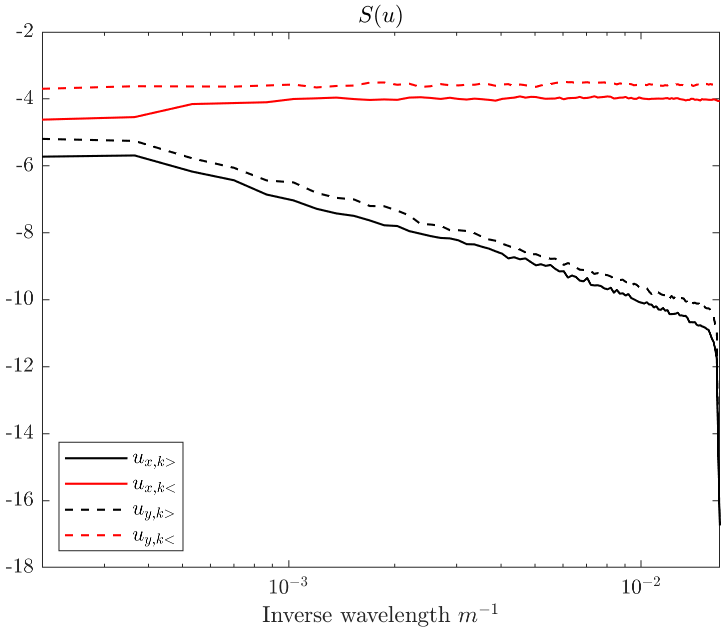
The results for the entropy are shown in Figure 11. We observed a decrease in the entropy for the small scales (black line), while for the large scales, the entropy quickly saturated (red line).
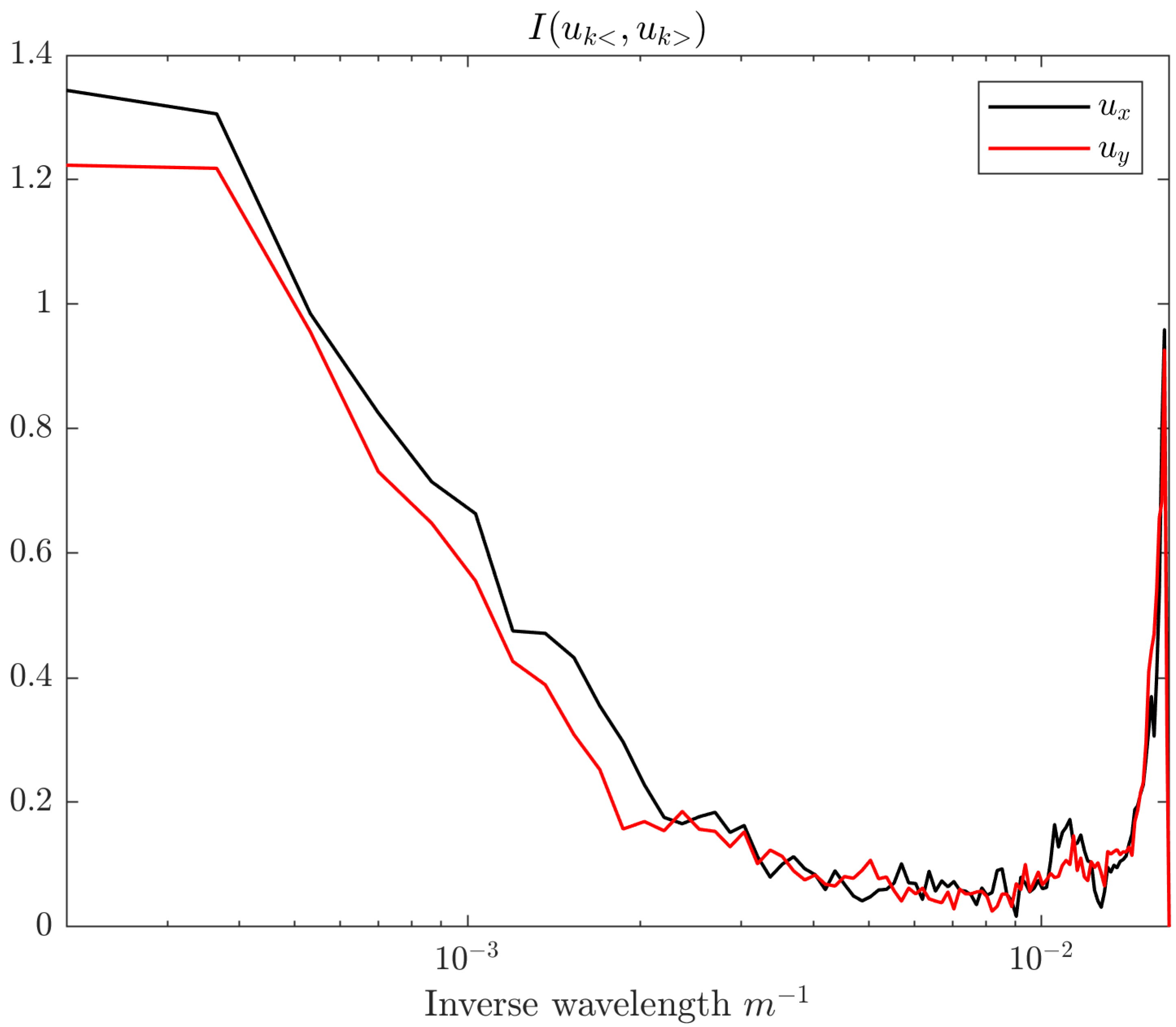
Figure 12 shows the mutual information between the filtered velocity fields. The apparent sharp increase in mutual information near the maximum wave number was probably due to the fact that we were approaching the minimum resolution of the simulation; so, this part of the result should not be considered reliable.
We observed a logarithmic decrease in entropy (note that the scale of the k axis is logarithmic); this behavior was previously observed in the inertial range [17]. In this case, we observed that the decrease in information was characterized by a slope of approx. , as shown in Figure 11. In the mutual information, we observed that a decoupling between the scales occurred at , which corresponded to a spatial scale of (remember that if the mutual information is in the order of 0, then the joint pdf of the system can be decomposed into a product ).
Previously, Shannon’s entropy has been interpreted as a system’s predictability [35]; in this sense, the largest scales are the least predictable. However, when complementing this interpretation with the mutual information, we see that at the large scales, more information was contained in the interactions, until the decoupling of the pdf occurred at small scales.
5. Summary and Conclusions
A modified state-of-the-art computational fluid dynamics code [21] was used as a framework to implement a highly resolved LES model of a midlatitude upper ocean front. Through numerical simulations, we investigated the spectral energy flux at the submesoscale/small-scale range in order to assess the inverse and forward kinetic energy fluxes at these scales and to inquire into the processes that drive them in the absence of any atmospheric forcing. At the surface, we found a strong direct kinetic energy flux. In this upper ocean region, the subgrid momentum diffusion was also intense. The computed deviation from the gradient wind balance showed that these processes were partially imbalanced, with some frontogenetic regions even exhibiting mostly balanced dynamics.
In deeper waters, the calculations predicted mostly an inverse kinetic energy flux. Deeper than 50 m, we did not observe submesoscale conditions, as , and the frontogenesis was almost imperceptible; at 75 m deep, there were only a few small regions with frontogenetic activity.
At the surface, the front showed significant coupling at scales larger than ∼10 (m). This was manifested as a strong direct energy cascade and intense communication between scales. At scales smaller than ∼ (m), the results showed near-zero energy flux, associated with weakly energetic coupled scales of motion; however, at the same scale range, the estimator of the mutual information flow still showed values that evidenced a significant level of communication between them. This motivates us to investigate the nature of the self-organized turbulent motion at this scale range with weak energetic coupling but where communication between scales is still significant and to inquire into the existence of synchronization or functional relationships between scales, with an emphasis on the eventual underlying nonlocal processes. This would enable creation of a more complex picture of the mechanics of turbulence as a property of self-organizing complex systems, the behavior of which would be characterized by processes involving the transfer of energy and information.
Author Contributions
Conceptualization, P.C.; Investigation, P.C. and A.B.; Writing—original draft, P.C. All authors have read and agreed to the published version of the manuscript.
Funding
This research was funded by the Interdisciplinary Center for Aquaculture Research (INCAR; FONDAP Project Number 15110027; CONICYT). The model simulations were run at the Laboratory of Computational Mechanics of the Department of Mechanical Engineering of the University of Concepción (Concepción, Chile).
Institutional Review Board Statement
Not applicable.
Data Availability Statement
The data presented in this study are available on request from the corresponding author.
Conflicts of Interest
The authors declare no conflict of interest.
Abbreviations
The following abbreviations are used in this manuscript:
| LES | Large Eddy Simulation |
| CFD | Computational Fluid Dynamics |
| SIMPLE | Semi-Implicit Method for Pressure-Linked Equations |
| KSG | Kraskov–Stögbauer–Grassberger |
| KL | Kozachenko–Leonenko |
References
- Sullivan, P.P.; McWilliams, J.C. Frontogenesis and frontal arrest of a dense filament in the oceanic surface boundary layer. J. Fluid Mech. 2018, 837, 341–380. [Google Scholar] [CrossRef]
- Nikurashin, M.; Vallis, G.K.; Adcroft, A. Routes to energy dissipation for geostrophic flows in the Southern Ocean. Nat. Geosci. 2012, 6, 48–51. [Google Scholar] [CrossRef]
- Shcherbina, A.Y.; D’Asaro, E.A.; Lee, C.M.; Klymak, J.M.; Molemaker, M.J.; McWilliams, J.C. Statistics of Vertical, Divergence, and Strain in a Developed Submesoscale Turbulence Field. Geophys. Res. Lett. 2013, 40, 4706–4711. [Google Scholar] [CrossRef]
- Capet, X.; McWilliams, J.C.; Molemaker, M.J.; Shchepetkin, A.F. Mesoscale to Submesoscale Transition in the California Current System. Part III: Energy Balance and Flux. J. Phys. Oceanogr. 2008, 38, 2256–2269. [Google Scholar] [CrossRef] [Green Version]
- McWilliams, J.C. Fluid Dynamics at the Margin of Rotational Control. Environ. Fluid Mech. 2008, 8, 441–449. [Google Scholar] [CrossRef]
- Thomas, L.N.; Tandon, A.; Mahadevan, A. Submesoscale Processes and Dynamics. In Ocean Modeling in an Eddy Regime; American Geophysical Union: Washington, DC, USA, 2008; pp. 17–38. [Google Scholar]
- Mahadevan, A.; Tandon, A.; Ferrari, R. Rapid changes in Mixed Layer Stratification Driven by Submesoscale Instabilities and Winds. J. Geophys. Res. 2010, 115, C03017. [Google Scholar] [CrossRef]
- Capet, X.; McWilliams, J.C.; Molemaker, M.J.; Shchepetkin, A.F. Mesoscale to Submesoscale Transition in the California Current System. Part II: Frontal Processes. J. Phys. Oceanogr. 2008, 38, 44–64. [Google Scholar] [CrossRef] [Green Version]
- Marino, R.; Pouquet, A.; Rosenberg, D. Resolving the Paradox of Oceanic Large-Scale Balance and Small-Scale Mixing. Phys. Rev. Lett. 2015, 114, 1–5. [Google Scholar] [CrossRef] [PubMed] [Green Version]
- Müller, P.; McWilliams, J.; Molemaker, J. Routes to Dissipation in the Ocean: The 2D/3D Turbulence Conundrum. In Marine Turbulence: Theories, Observations and Models; Cambridge University Press: Cambridge, UK, 2005; pp. 1–23. [Google Scholar]
- Lévy, M.; Ferrari, R.; Franks, J.; Martin, A.P.; Riviere, P. Bringing Physics to Life at the Submesoscale. Geophys. Res. Lett. 2012, 39, 1–41. [Google Scholar] [CrossRef] [Green Version]
- Hoskins, B.J.; Bretherton, F. Amospheric Frontogenesis Models: Mathematical Formulation and Solution. J. Atmos. Sci. 1972, 29, 11–37. [Google Scholar] [CrossRef]
- Hoskins, B.J. The Mathematical Theory of Frontogenesis. Annu. Rev. Fluid Mech. 1982, 14, 131–151. [Google Scholar] [CrossRef] [Green Version]
- Lee, C.; Rainville, L.; Harcourt, R.; Thomas, L. Enhanced Turbulence and Energy Dissipation at Ocean Fronts. Science 2011, 332, 318–322. [Google Scholar]
- Nagai, T.; Tandon, A.; Yamazaki, H.; Doubell, M.J. Evidence of Enhanced Turbulent Dissipation in the Frontogenetic Kuroshio Front Thermocline. Geophys. Res. Lett. 2009, 36, 1–6. [Google Scholar] [CrossRef]
- Cerbus, R.; Goldburg, W. Information content of turbulence. Phys. Rev. E 2013, 88, 053012. [Google Scholar] [CrossRef] [PubMed] [Green Version]
- Granero-Belinchón, C.; Roux, S.G.; Garnier, N.B. Kullback-Leibler divergence measure of intermittency: Application to turbulence. Phys. Rev. E 2018, 97, 013107. [Google Scholar] [CrossRef] [Green Version]
- Granero-Belinchon, C.; Roux, S.G.; Garnier, N.B. Scaling of information in turbulence. EPL Europhys. Lett. 2016, 115, 58003. [Google Scholar] [CrossRef] [Green Version]
- Lozano-Durán, A.; Arranz, G. Information-theoretic formulation of dynamical systems: Causality, modeling, and control. Phys. Rev. Res. 2022, 4, 023195. [Google Scholar] [CrossRef]
- Wang, W.; Chu, X.; Lozano-Durán, A.; Helmig, R.; Weigand, B. Information transfer between turbulent boundary layers and porous media. J. Fluid Mech. 2021, 920. [Google Scholar] [CrossRef]
- Cornejo, P.; Sepúlveda, H. Computational Fluid Dynamics Modelling of a Midlatitude Small scale Upper ocean front. J. Appl. Fluid Mech. 2015, 9, 1851–1863. [Google Scholar] [CrossRef]
- Smagorinsky, J. General Circulation Experiments with the Primitive Equations. I. The Basic Experiment. Mon. Weather Rev. 1963, 91, 99–164. [Google Scholar] [CrossRef]
- Scotti, A.; Meneveau, C.; Lilly, D.K. Generalized Smagorinsky Model for Anisotropic Grids. Phys. Fluids A Fluid Dyn. 1993, 5, 2306–2308. [Google Scholar] [CrossRef]
- Stone, P. On the Geostrophic Baroclinic Stability. J. Phys. Oceanogr. 1966, 23, 390–400. [Google Scholar] [CrossRef]
- Stone, P. A Simplified Radiative-dynamical Model for the Static Stability of Rotating Atmospheres. J. Atmos. Sci. 1972, 29, 405–418. [Google Scholar] [CrossRef]
- McWilliams, J.C. A Uniformly Valid Model Spanning the Regimes of Geostrophic and Isotropic, Stratified Turbulence: Balanced Turbulence. J. Atmos. Sci. 1985, 42, 1773–1774. [Google Scholar] [CrossRef]
- Skyllingstad, E.D.; Samelson, R.M. Baroclinic Frontal Instabilities and Turbulent Mixing in the Surface Boundary Layer. Part I: Unforced Simulations. J. Phys. Oceanogr. 2012, 42, 1701–1716. [Google Scholar] [CrossRef]
- Kozachenko, L.F.; Leonenko, N.N. Sample estimate of the entropy of a random vector. Probl. Peredachi Informatsii 1987, 23, 9–16. [Google Scholar]
- Kraskov, A.; Stögbauer, H.; Grassberger, P. Estimating mutual information. Phys. Rev. E 2004, 69, 066138. [Google Scholar] [CrossRef] [Green Version]
- Charney, J.G. Geostrophic Turbulence. J. Atmos. Sci. 1971, 28, 1087–1095. [Google Scholar] [CrossRef]
- Blumen, W. Uniform Potential Vorticity Flow: Part I. Theory of Wave Interactions and Two-Dimensional Turbulence. J. Atmos. Sci. 1978, 35, 774–783. [Google Scholar] [CrossRef]
- Capet, X.; Klein, P.; Hua, B.L.; Lapeyre, G.; Mcwilliams, J.C. Surface Kinetic Energy Transfer in Surface Quasi-geostrophic Flows. J. Fluid Mech. 2008, 604, 165–174. [Google Scholar] [CrossRef] [Green Version]
- Boyd, J.P. The Energy Spectrum of Fronts: Time Evolution of Shocks in Burgers’ Equation. J. Atmos. Sci. 1992, 49, 128–139. [Google Scholar] [CrossRef]
- Higgins, C.; Parlange, M.B.; Meneveau, C. Energy issipation in Large-Eddy Simulation: Dependence on Flow Structure and Effects of Eigenvector Alignments. In Atmospheric Turbulence and Mesoscale Meteorology; Cambridge University Press: Cambridge, UK, 2004; pp. 51–70. [Google Scholar]
- Holloway, G. Eddies, waves, circulation, and mixing: Statistical geofluid mechanics. Annu. Rev. Fluid Mech. 1986, 18, 91–147. [Google Scholar] [CrossRef]
Figure 1.
The computational model. The grid and dimensions (top) and the initial density distribution (bottom).
Figure 1.
The computational model. The grid and dimensions (top) and the initial density distribution (bottom).

Figure 2.
The relationship between entropy and mutual information.

Figure 3.
The submesoscale structures ( iso-surface) within the mixed layer. The planes at the depths of 25 m (red), 50 m (green), and 75 m (blue).
Figure 3.
The submesoscale structures ( iso-surface) within the mixed layer. The planes at the depths of 25 m (red), 50 m (green), and 75 m (blue).

Figure 4.
The velocity field at the depths of 25 m (left), 75 m (middle), and 300 m (right). The structures in grey are the projections of the isosurface.
Figure 4.
The velocity field at the depths of 25 m (left), 75 m (middle), and 300 m (right). The structures in grey are the projections of the isosurface.

Figure 5.
The Rossby number distribution at the depths of 25 m (left), 75 m (middle), and 300 m (right).
Figure 5.
The Rossby number distribution at the depths of 25 m (left), 75 m (middle), and 300 m (right).

Figure 6.
The 1D kinetic energy and available potential energy wave number spectra along the front.

Figure 7.
The kinetic energy flux.

Figure 8.
The subgrid momentum diffusion distribution at the depths of 25 m (left), 75 m (middle), and 300 m (right).The isosurface projection is shown as a grey region.
Figure 8.
The subgrid momentum diffusion distribution at the depths of 25 m (left), 75 m (middle), and 300 m (right).The isosurface projection is shown as a grey region.

Figure 9.
The error in the wind gradient balance at the depths of 25 m (left), 75 m (middle), and 300 m (right). The isosurface projection is shown as a grey region.
Figure 9.
The error in the wind gradient balance at the depths of 25 m (left), 75 m (middle), and 300 m (right). The isosurface projection is shown as a grey region.

Figure 10.
The frontogenesis factor at the depths of 25 m (left), 75 m (middle), and 300 m (right). The isosurface projection is shown as a grey region.
Figure 10.
The frontogenesis factor at the depths of 25 m (left), 75 m (middle), and 300 m (right). The isosurface projection is shown as a grey region.

Figure 11.
The entropy distribution.

Figure 12.
The mutual communication between scales.

Disclaimer/Publisher’s Note: The statements, opinions and data contained in all publications are solely those of the individual author(s) and contributor(s) and not of MDPI and/or the editor(s). MDPI and/or the editor(s) disclaim responsibility for any injury to people or property resulting from any ideas, methods, instructions or products referred to in the content. |
© 2023 by the authors. Licensee MDPI, Basel, Switzerland. This article is an open access article distributed under the terms and conditions of the Creative Commons Attribution (CC BY) license (https://creativecommons.org/licenses/by/4.0/).
Share and Cite
MDPI and ACS Style
Cornejo, P.; Bahamonde, A. Energy and Information Fluxes at Upper Ocean Density Fronts. Fluids 2023, 8, 17. https://doi.org/10.3390/fluids8010017
AMA Style
Cornejo P, Bahamonde A. Energy and Information Fluxes at Upper Ocean Density Fronts. Fluids. 2023; 8(1):17. https://doi.org/10.3390/fluids8010017
Chicago/Turabian StyleCornejo, Pablo, and Adolfo Bahamonde. 2023. "Energy and Information Fluxes at Upper Ocean Density Fronts" Fluids 8, no. 1: 17. https://doi.org/10.3390/fluids8010017