Article

Unsteady Fluid Flows in the Slab Mold Using Anticlogging Nozzles

by
María Guadalupe González-Solórzano
1,*,
Rodolfo Morales Dávila
1,
Javier Guarneros
2,
Ismael Calderón-Ramos
3,
Carlos Rodrigo Muñiz-Valdés
4 and
Alfonso Nájera-Bastida
5
1
Department of Metallurgy, Instituto Politécnico Nacional-ESIQIE, Ed. 7, Zacatenco, Mexico City 07738, Mexico
2
K&E Technologies, Manizalez 88, San Pedro Zacatenco, Mexico City 07365, Mexico
3
Mechanics Engineering Department, Universidad Autónoma de Coahuila-FIME-UN, Barranquilla S/N, Col. Guadalupe, Monclova Coahuila 25750, Mexico
4
Facultad de Ingeniería, Universidad Autónoma de Coahuila, Blvd. Fundadores km 15 13, Ciudad Universitaria, Arteaga Coahuila 25350, Mexico
5
Instituto Politécnico Nacional-UPIIZ, Metallurgy Engineering, Blvd. Del Bote 202, Cerro del Gato, Zacatecas 98160, Mexico
*
Author to whom correspondence should be addressed.
Fluids 2022, 7(9), 288; https://doi.org/10.3390/fluids7090288
Submission received: 11 July 2022 / Revised: 6 August 2022 / Accepted: 7 August 2022 / Published: 30 August 2022
(This article belongs to the Special Issue Modelling and Simulation of Turbulent Flows)

Abstract

:
The characterization of the fluid flow of liquid steel in a slab mold, using two nozzle designs under unclogged and clogged conditions, is performed using physical and mathematical simulations. Nozzle A, with an expanding and contracting geometry, yields larger sub-meniscus experimental velocities than nozzle B, with internal flow deflectors. The numerical predictions indicate quick time-changing velocity profiles in the submeniscus region between the mold’s narrow face and the nozzles. The flow deflectors in nozzle B have two effects; the high dissipation rate of kinetic energy in the upper-half length induces lower velocities in the ports than nozzle A. The neutralization of the biased flow caused by the sliding gate allows a balanced fluid through the ports. According to the results, nozzle A yields velocity profiles in the sub-meniscus region with larger standard deviations than nozzle B, leading to an unstable bath surface. The clogged nozzles produced biased-asymmetrical flow patterns in the mold, finding approximated matchings between numerical predictions and experimental measurements. The internal protrusions of the deposits lead to covariance losses of the bath surface wave heights. The use of internal deflectors helped to decrease the amount of clog material in nozzle B.

Graphical Abstract

1. Introduction

The fluid flow of liquid steel in slab continuous casting molds is one of the most challenging phenomena to understand. The flow regime is turbulent inside the nozzle or submerged entry nozzle (SEN) and the mold. The effects of the two discharging jets yield a liquid steel meniscus of a high turbulence region because of the receiving of the upper rolls flows. Depending on the mold dimensions, steel throughput, nozzle immersion depth, and nozzle design, the general flow pattern of steel in the mold can be double roll, double roll-medium flow, single roll, or unstable flow (see Figure 1). The first flow pattern ensures a trend of symmetric heat transfer and a steady solidifying shell downwards from the mold that the other three flows cannot provide. However, a free defects slab is impossible, even with a double roll flow pattern. For example, the uncontrolled liquid flow near the metal-flux interface, characterized by high velocities and vortexes, will cause powder entrainment to become trapped particles (inclusions) in the solidified shell [1,2]. If the upper flow delivers cold steel, it will not be enough to melt the mold flux. The non-melted powder induces sticking breakouts and bath level oscillations, promoting transversal slab depressions [3,4,5,6]. A criterion establishes that the maximum melt velocity of 0.3 m/s at the melt-flux interface, for any given casting speed, avoids flux entrapment and the generation of slivers [7,8]. In other words, the flow along the steel-slag interface generates shear stresses, velocity, bumps, and waves, leading to finger-like protrusions of liquid slag into steel. These bumps and protrusions of liquid slag disintegrate into slag droplets following the flow in the liquid steel in the mold. Other entrainment mechanisms are through fluid flow vortexing, sucking the mold flux particles, and forming droplets in the melt bulk [9]. These entrained droplets can finally form nonmetallic inclusions in the steel material, causing defects in the final product such as slivers and laminations, and, therefore, they should be avoided.
When the flow is unstable and asymmetric (see Figure 1b–d), one of the two jets of the bifurcated SENs yields higher velocities, increasing the asymmetric turbulence, enhancing the flux entrainment, and disturbing the heat transfer uniformity through the copper plates. With large flows of argon, excess motion around the SEN leads to its severe erosion, forming a stressed nozzle neck that eventually might fracture it [9]. On the contrary, a lack of movement between the SEN outer wall and the mold wall will freeze the steel, forming thick shells subjected to thermal stresses that may exceed its strength and produce longitudinal cracks on the slab surface [10,11]. The industrial experience indicates that a hot meniscus ensures a better slab surface, with minor defects such as slivers, cracks, slag entrapment, and transversal depressions [12,13,14]. A hot meniscus is particularly important in casting Stabilized Ultra-Low Carbon Steels (SULC) and peritectic steels [15,16]. The use of argon aims to decrease the clogging of the nozzles or SENs by forming a gaseous layer on the interior wall to keep away the alumina particles and force them to flow in the mainstream of liquid steel. However, argon usage frequently brings about more problems than solutions. The control of the argon flow rates must align with the steel throughput. Low steel throughputs and high argon flow rates lead to excessive slag foaming close to the nozzle driven by large gas bubbles and the slipping of slag films on the surface. Once having reached the port, these slag films fragment and become particles entrained in the liquid bulk by the discharging jet [17,18] to ultimately end in particles trapped by the mushy regions of the solidifying shell. High steel throughputs and small gas flow rates result in tiny bubbles transported to the shell and trapped by the dendritic structure. These bubbles trap inclusions and, once in the shell, become small cavities surrounded by inclusions. During the rolling process, these defects have the assigned name of pencil pipes, and during the sheet annealing process, their presence becomes evident thanks to their inflation-forming blisters [19,20]. Although there are published criteria by which to use the balanced flow rates of argon with steel throughput [21,22,23], very few plants apply the balanced argon operation.
Therefore, a more appropriate SEN design must deliver hot steel to melt the mold powder with minimum flux entrainment, forming a double roll flow pattern and minimum variations of the meniscus levels. The double roll flow pattern must prevail throughout the casting time, maintaining a stable shear flow without vortexing at and below the meniscus. Additionally, this nozzle must operate free of argon to avoid all the operational and product quality inconveniences generated by this practice. Any SEN design fulfilling these conditions will guarantee an excellent performance under industrial operating conditions.
The present work deals with the fluid flow characterizations in a slab mold using two different anticlogging SEN designs. In an anti-clogging nozzle, the raw material is isostatically pressed to conform to a solid piece with a surface treatment to decrease the adherence of alumina inclusions on the internal wall of the SEN [24,25]. These anticlogging nozzles operate without argon bubbling.
Both nozzles operate in two slab casters in the US with no argon bubbling in the nozzle. This work’s objective is to evaluate the stability of the fluid flow pattern, the variations of the meniscus levels, and the meniscus stability under free flow and clogging conditions. The application of physical and mathematical approaches is the appropriate path to adopt. The following sections explain the experimental and mathematical models and the discussions associated with the results obtained through these two approaches.

2. Experimental Work

A full-scale mold model made of 15 mm-thick transparent plastic sheets with dimensions 250 × 1450 mm2 and a length of 1700 mm serves as the experimental tool of this research. A total of 200 mm of the mold bottom remain inside a water tank (2.2 m deep) surrounded in the bottom by a 10 mm-thick steel plate to keep the mold fixed and immobile. A perforated plate of the same plastic sheets covers the end of the plastic mold to control the downflow of water. Inside the water tank, an immersed pump sends the water to a tundish with a constant water level of 1 m. In the pipe that transports water from the tank to the tundish, there is a flow-controlling valve and a flow meter; both devices help maintain the liquid throughput fed in the tundish. Replicas of the industrial upper tube nozzle, UTN, and sliding gate, made of plastic, control the casting speed. A steel frame in the mold top holds six ultrasonic sensors whose tips are 120 mm above the static water level, three at each side of the nozzle, sending ultrasonic signals to the bath surface. A data acquisition card converts the reflected analogical ultrasonic signals to digital ones permitting the real-time recording of the water instantaneous levels by plotting them against the measuring time. An ultrasonic transducer with a frequency of 1 × 10⁷ Hz located 20 mm below the meniscus in the midface of the narrow mold wall captured the instantaneous velocities and all turbulence statistics for further analysis. Figure 2 shows a scheme of the mold and the ultrasonic sensors with their respective positions in the middle of the mold thickness, Figure 3a shows a general view of the mold with the level sensors in the top, and Figure 3b shows the bottom of the tundish, the Upper Tube Nozzle, UTN, and the sliding gate.
Figure 4a,b show the designs of these SENs, named A and B. The first consists of a body with one expansion and one contraction of the cross-section area or bore, with two 25° ports. The second has four internal ring-deflectors to control the internal turbulence and to decrease the biased flow originating from the sliding gate aperture. The angle of the ports is 25°. Both nozzles have quite different designs, making them worth comparing to unveil the different flows in the slab mold. The manufacturing of the models of these two SENs consisted of machining nylon-polyamide bars for the internal and outer surfaces of the bodies. The 3D printing technology helped to manufacture the corresponding SEN tips. The two SEN bodies consist of three pieces plus the tips to assemble and disassemble them, as required. The threaded end of the bodies and the threaded upper sides of the tips are screwed to constitute solid SEN pieces. The activities at the caster consisted of making a simultaneous trial of both nozzles in a two-strands tundish, operating one strand with nozzle A and the other strand with nozzle B. The casting sequence lasted four hours when the clogging index detected the incoming fluid flow disturbances, as confirmed by the mold’s heat transfer flux variations. The clogged nozzles were extracted from the tundish to manufacture the corresponding models following the procedure explained below:
  • A resin poured in the used nozzles permitted the capture of the topography of the clog surfaces adhering to the interior surfaces of the two industrial SENs. The solidified pieces work as cores (see Figure 5).
  • The next step consists of cutting the industrial SENs along their lengths, yielding two halves, using a circular saw to extract the cores from the nozzles.
  • Each nozzle is composed of a body, split in two halves and previously machined, and a 3D-printed tip with two bifurcated ports. Figure 5 shows the dissembled nozzles.
  • The wrapped extracted core with the pieces of each disassembled model, including the tips of each SEN, conformed to a new casting system. With the core fixed into the assembled nozzle, there is a gap left between the clog and the core.
  • A liquid rubber poured in the new casting filled the gap left between the nozzle surface and the core, forming an exact replica of the clog’s topography.
  • By disassembling the nozzle, the core is again taken out; a final reassembling operation of the model nozzle yields a replica of the actual nozzle, with its respective alumina clogging adhering to the interior walls.
  • A laser scanner introduced inside each assembled nozzle model, with their respective clog-models, supplied digital files of the surface’s topographies. These digital files were later used in building the computational meshes of the mathematical models.
Figure 4. Geometric features of the nozzles. (a) Nozzle A. (b) Nozzle B.
Fluids 07 00288 g004
The bores of the bodies of both nozzles have diameters 1.0 mm larger than the original ones indicated in the blueprints. This machining operation compensates for the gap’s interface thickness between the nozzle’s interior surface and the rubber, modeling the presence of the clogs. Figure 5a,b show the nozzle A and nozzle B models, respectively. It is remarkable that nozzle B has a layer of alumina along its length and in the port, while nozzle B shows clogging only in the region of the ports; the body is alumina-free.
An experiment started by opening the water valves and adjusting the flow rates and bath levels, continuing for 20 min to obtain a steady operation. At an arbitrary time, after the first 20 min, a red dye tracer injected in the UTN facilitated the recording of the mixing process by a conventional video camera. The video recording revealed the overall flow patterns using both nozzles. Finally, by putting the ultrasonic transducer into operation to record the turbulence statistics, the ultrasonic level sensors complete one experimental cycle, which is repeated until the experimental program is completed. Table 1 shows the experimental activities performed in this research.

3. Mathematical Model

The mathematical simulation was carried out with the ANSYS Fluent software (Fluent 17.2, ANSYS Inc., Centerra Resource Park, Lebanon, 2016). The mathematical model consists of an Unsteady Reynolds-Averaged Navier Stokes (URANS) computational scheme based on the realizable k-ε model [26]. The realizable k-ε turbulence model is simple, contains an alternative formulation for the turbulent viscosity, and predicts the boundary layer characteristics under large pressure gradients. The realizable model provides the best performance of all the k-ε model versions for several conditions of separated flows and flows with complex secondary flow features [27]. The equations governing the motion of an incompressible fluid include one equation for continuity and three equations for momentum transfer, expressed by averaging on time according to the Reynolds decomposition ( u i = u i + u ¯ i ),
u i ¯ x i = 0
u ¯ i t + u ¯ i u ¯ j x j = 1 ρ p x i + ν 2 u ¯ i x i x j + 1 ρ τ i j R x j + ρ g i
The Reynolds stresses, τ R = u i u j ¯ , are approximated through the hypothesis of the eddy viscosity, μ t , according to the Boussinesq expression,
τ i j R = 2 μ t + 2 S i j 2 3 k δ i j
where Sij is the mean deformation rate tensor (see Equation (8) below). The relation between the eddy or turbulent viscosity and the kinetic energy ( k = 1 2 u i u j ¯ ) and the dissipation rate of this energy, ε, is:
ν t = C μ ρ k 2 ε
Cμ is a function of the mean strain and rotation rates, the angular velocity of the system, and the turbulence fields of k and ε.
C μ = 1 A 0 + A s k U ε
where
U = S i j S i j + Ω ˜ i j Ω ˜ i j
Ω ˜ i j = Ω i j 2 ϵ i j k ω k
A0 = 0.04, A s = 6 cos ϕ and
ϕ = 1 3 c o s 1 6 W   a ,   W = S i j S j k S k i S ˜ 3   b ,   S ˜ i j = S i j S i j   c ,   S i j = 1 2 u j x i + u i x j   d
The variable Cμ in Equations (4) and (5) recovers the standard constant value of 0.09 for an inertial sublayer in an equilibrium boundary layer.
The model simulates the fields of the kinetic energy and its dissipation rate to calculate the eddy viscosity by solving the k and ε balances,
k t + · u ¯ k = τ R : u ¯ ε + · ν + ν t σ k k
ε t + · u ¯ ε =   C ε 1 ε k + C 1 S i j ε C ε 2 ε 2 k + v ε + · ν + ν t σ ε ε
where C 1 = max 0.43 ,   η η + 5 , S = 2 S i j S i j and C ε 1 = 1.44 ,   C ε 2 = 1.9 ,   σ k = 1.0 ,   σ ε = 1.2 .
η = S k ε
The no-slipping boundary condition applies to all walls in the system, and the link between the wall and the outer flow, from the boundary layer, is through the Log-Law wall function [28]. At the nozzle inlet, the velocity-inlet boundary condition is applied, and at the bottom of the mold, the pressure-outlet condition is applied. To take into account the presence of the upper-layer phase, the shear boundary condition applies on the bath surface. The computing mesh and the numerical parameters are in Table 2. Figure 6a,b show the computational mesh of the unclogged nozzles A and B, respectively, and Figure 6c,d show the corresponding computational meshes of the clogged nozzles A and B, respectively. The mathematical simulation time corresponds to 300 s.

4. Results and Discussion

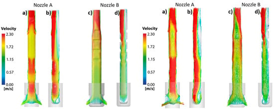
4.1. Fluid Flow Using Unclogged Nozzles

In the following lines, the description and discussion make indistinct use of the physical and mathematical results alike. This discussion approach permits a versatile way to handle data.
Figure 7 and Figure 8 show the double-roll flow patterns yielded by both nozzles despite their shallow immersion. Both flows show acceptably symmetry; this statement is supported by the numerical predictions in the symmetric-longitudinal planes seen in Figure 7d and Figure 8d for nozzles A and B, respectively. Table 3 shows the time spent by the discharging jets, determined by the mixing front of the tracer and counted from the nozzle ports until touching their outer nozzle’s outer wall driven by the upper roll flow. From these times, it is evident that the liquid velocity along the meniscus level is slightly higher using nozzle A than it is through using nozzle B. The meniscus surface shows the effects of the velocity differences between the two nozzles by its deformation indicated by the arrows in Figure 7b,c when using nozzle A.
Figure 8a–c show a flat meniscus, indicating a region with fewer stirring conditions provided by nozzle B. Figure 9a–c show the quantitative evaluation of the meniscus level deformation reported through the bath level variations. The bath level variations, named wave height (WH), help to quantify the meniscus stability. When using nozzle A, there is a gap in the bath level oscillations or WH between the two extremes of the mold indicated by sensors 1 (extreme right side) and 6 (extreme left side). The magnitudes of these WHs (wave heights) are as high as 15 mm and as low as −25 mm due to the high subsurface liquid velocities detected by sensor 6. In the regions between the narrow mold face and the nozzle (middle regions, monitored by sensors 2 and 5), the wave gaps between positions 2 and 5 and the WHs decrease, indicating a relative dynamic matching of the oscillations between the middle groups’ positions. However, in the two regions beside the nozzle (monitored by sensors 3 and 4), the gap magnitudes and the WHs increase considerably, yielding magnitudes as high as 14 mm and as low as −30 mm, with reference to the static bath level. Thus, the liquid accelerates before impacting the nozzle’s outer wall. The covariances between the oscillations of each pair of sensors are shown in Figure 10a. These covariances, detected through all sensors, are positive and significant, varying between 20 and 27, indicating a direct correlation between the flow events and wave motions at each side of the nozzle. Figure 9d–f show the quantitative evaluation of the meniscus level deformation through the WHs using nozzle B. Unlike the level oscillations yielded by nozzle A, nozzle B yields considerably smaller WHs with slight gaps between the wave signals detected by each pair of sensors. The most significant oscillations or wave gaps are detected by sensors 1 and 6, i.e., the two extremes of the mold. As the variances of the oscillation amplitudes or WH are small, so are the covariances, though there is a small negative covariance between sensors 3 and 6 (see Figure 10b). It is worth noting that, for conversion, the WHs reported in Figure 9 should be multiplied by a factor of 0.59 to account for the significant differences in physical properties between water and steel (see Appendix A).
Figure 11 and Figure 12 show the numerical unsteady velocity fields provided using nozzles A and B, respectively. As seen in Figure 11a–d, nozzle A maintains the flow symmetry for a long time. When the symmetry partially vanishes, as seen in Figure 11e, it is rapidly recovered after a few seconds (see Figure 11f). On the other hand, at some given time, nozzle B shortens the upper roll flows (Figure 12a,b) without losing symmetry. The flows recover their symmetry (Figure 12c), with periods of losses and gains of symmetry, but maintain the flow stability throughout the casting time.
It is worth mentioning that most researchers [31,32,33,34,35,36] report averaged parabolic-like velocity profiles in the subsurface region between the narrow mold face and the outer nozzle’s wall. These velocity profiles are important because, if the peak velocity in the sub-meniscus regions is higher than a given critical magnitude, the flow will entrain the mold flux particles inside the liquid bulk. However, conclusions based on such velocity profiles may be misleading since the actual conditions show wide time-dependent variations. Figure 13a,c show the Probability Density Functions (PDF) of the experimental velocities for nozzles A and B, respectively. Nozzle A yields negative velocities (liquid flowing from the nozzle toward the narrow mold face) that the numerical model does not predict. However, most instantaneous numerical velocity profiles fall in the gray area corresponding to the standard deviation of the experimental measurements. Nozzle B yields only positive velocities, and the numerical and the measured instantaneous velocity profiles fall in the gray area. Figure 13b,d show the numerical velocity profiles (each profile corresponds to periods of one second, demonstrating the wide variations within short times) and experimental measurements of the velocities corresponding to the left sides of nozzles A and nozzle B, respectively. The green lines in these plots are the averages of the measured velocities, and the gray areas correspond to the standard deviations of each recorded velocity in the field at a given distance. These plots also show the numerical velocity profiles at different times, overlapping the experimental measurements.
A comparison between both types of data leads to the following observations:
  • The experimental velocities obtained using nozzle A include wide variations, reporting even negative velocities. The numerical results remain embodied inside the gray band region, lacking any numerical predictions with negative velocities.
  • The numerical and experimental results yield radical time-changing velocity profiles, emphasizing the turbulent nature of the flow.
  • The experimental velocities obtained using nozzle B yield a narrower band of variations, and the numerical results show some profiles outside, upwards in the region close to the SEN. However, some other instantaneous numerical results fall inside the gray experimental band, matching the experimental measurements well.
  • The peak or spike velocities, predicted numerically for both nozzles, change to different positions between the narrow mold face and the nozzle, with time seldom falling in the middle position between the narrow mold wall and the outer nozzle’s wall.
  • The numerical and experimental magnitudes of the velocity profiles are smaller in the flows yielded by nozzle B than in those yielded by nozzle A.
  • The numerical predictions broadly predict the experimental measurements matching the overall dynamics of the subsurface flow.
The mold inherits its flow patterns from those corresponding in the interiors of the nozzles providing velocity spikes to the mold flow that produce and dissipate energy [37,38]. These internal flows are seen in Figure 14a,b for unclogged nozzle A and in Figure 14c,d for unclogged nozzle B. The flow inside nozzle A observes a biased flow. Internal velocities are as high as 2.3 m/s due to the partial opening of the sliding gate. The fluid in this nozzle is accelerated and decelerated by contractions and expansions of the bore. The discharging flow impacts the nozzle bottom with velocities of 0.6–1.3 m/s.
On the other hand, the biased flow is practically eliminated by the internal deflectors in nozzle B, providing velocities between 0.5 (in the bottom) and 2.3 m/s in the nozzle top (see Figure 14c,d). The kinetic energy dissipation rates for nozzles A and B are seen in Figure 15a–d, respectively. The dissipation rates are larger in nozzle B due to the impact of the fluid on the internal deflectors. Hence, the lower discharging velocities in the ports of nozzle B are related to the dissipation rate level of turbulent energy in the upper region. Figure 16a–d show the discharging velocities in the ports of nozzles A and B. Figure 16a,b show the port area utilization of nozzle A, which is constrained in a minimal area with velocities as high as 1.5 m/s located in the opposed bottom corners of the left and right ports. Therefore, each jet orientates towards one of the two broad mold faces after leaving the nozzle. The port utilization of nozzle B is larger than that of nozzle A due to the elimination of the internal biased flow with maximum liquid velocities of about 1.2 m/s in the discharging ports.

4.2. Fluid Flow Using Clogged Nozzles

Figure 17a–d show the flow pattern using clogged nozzle A, where the left jet flows downwards and the right jet flows upwards, providing a very asymmetric mixing of the tracer. The flow pattern predicted by the mathematical model in Figure 17d matches the trajectories of the discharging jets outlined by the red dye tracer reasonably well. The flow in the left side of the nozzle is quite complex, with a region of small velocities close to its outer wall. A well-stabilized vortex flow in the mold corner is caused by the shearing flow coming from the port’s upper edge. On the right side, there is a well-defined upper roll flow. Figure 18a–d show the flow pattern using clogged nozzle B, where the right jet forms and flows upwards; on the other hand, the left jet flows downwards, providing a very asymmetric mixture of the tracer. Figure 18d shows the flow pattern predicted by the mathematical model. There is a well-developed upper roll flow on the right side, and on the left side, there is a sizeable stagnant region.
Figure 19a–c show the corresponding meniscus level oscillations or WHs using nozzle A, finding significant variations with time. The WHs reported by each pair of sensors vary between 30 and −35 mm. Thereby, the right side of the meniscus shows extreme turbulence conditions due to the well-developed double roll flow (see sensors 1–3). On the left side, the sizeable stagnant region yields WHs of low amplitude (see sensors 4–6). In Figure 19d–f, there are the corresponding WHs for the pairs of sensors at each side of the nozzle using nozzle B. The gaps among the WHs, corresponding to nozzle B, are appreciable in the oscillations reported by sensors 1 and 6 at the two extremes of the mold and sensors 3 and 4, i.e., in the two regions closer to the outer nozzle’s wall. Thus, both nozzles yield decoupled flows on both sides, revealing the non-symmetric flows derived from the clogging conditions. As mentioned with Figure 9, the WH’s in Figure 19 must also be multiplied by the factor of 0.59 to account for the significant differences in physical properties between water and steel.
The WHs covariances of the clogged nozzles A and B are in Figure 20a,b, respectively. The magnitudes of covariance of nozzle A decrease considerably, indicating that the phasing off the WHs between each pair of sensors includes some negative magnitudes indicating opposing directions of the oscillations (pairs 1–2, 1–3, 2–4, 2–5, 3–4, and 4–6). On the other hand, the oscillation events in both sides of nozzle B keep positive correlations even under clogged conditions.
The clogging profoundly alters the internal flows in the nozzles; Figure 21a–d show the velocity vectors observing highly biased conditions, and, different from the unclogged case, the liquid flows along the nozzle at high velocities close to the wall due to the obstructions. The jets, leaving nozzle A, are constrained to narrow jets in the nozzle bottom, reaching velocities close to 2.0 m/s, as seen in Figure 21a. Figure 21b shows a long recirculating flow with small velocities. This flow is opposed to the downwards high-velocity flow from the sliding gate aperture. This region also exists in unclogged nozzle A, though there is a defined recirculation flow in that case. Unlike nozzle A, nozzle B yields an unbiased and symmetric flow, as seen in Figure 21c,d, because the internal deflectors control the flow even under the clogging condition. The flows through the ports look more distributed in this nozzle than in nozzle A. Figure 22b,d show the instantaneous experimental and numerical velocities for the clogged nozzles A and B, respectively. In the case of nozzle A, the numerical predictions are in a narrow band of velocities falling well inside the broad gray area corresponding to the standard deviations of the measurements. Indeed, the numerical predictions indicate peak velocities that are considerably smaller than the measured velocity peaks (see the corresponding PDF; Figure 22a). As seen in Figure 22d for nozzle B, there is a mismatch between the experimental negative velocity measurements and the numerical predictions verified by the corresponding PDF in Figure 22c. The numerical results predict a narrow band of numerical instantaneous velocity profiles with small magnitudes, while the experimental measurements report essentially negative magnitudes. A possible reason for this disagreement is that the ultrasound transducer measures only the unidirectional velocity changes. Since the flow in this region is quite complex, including vortexes and recirculations, the equipment detects them as negative magnitudes. Figure 23a–d report these subsurface flows. Figure 23a shows the velocity fields using nozzle A. Figure 23b shows the velocity field corresponding to nozzle B. These instantaneous flows show an asymmetry with positive velocities (liquid flowing from the narrow mold face toward the outer nozzle’s wall). The flow asymmetry intensifies with the clogged nozzles, though the velocities are positive using nozzle A (see Figure 23c), matching the experimental results reported in Figure 22b. However, the flow in the left side of the mold, using nozzle B, yields vortexes and recirculations (see Figure 23d). Figure 24a–d show this complex flow’s evolution with time, using nozzle B, finding a crossed flow of liquid with a higher momentum on the right side transferring momentum to the left side. When the right flow surrounds the nozzle, a vortex is formed beside the left side of the nozzle’s wall, generating secondary vortexes, as seen in Figure 24a,b. At other times, the liquid velocities in the gap between the mold wall and the nozzle’s outer wall generate large vortexes, changing the directions of the velocity vectors near the mold’s narrow face (see Figure 24c,d).
The water model in Figure 25a–d shows the velocity fields at different times and precisely replicates the flows described above when the mold operates with nozzle B. The liquid on the right side forms a double roll flow, while a weakened flow impacts the left narrow mold face (see Figure 25a,b). Figure 25c shows the upper flow’s advance indicated by arrow 1, making the weakened flow from the left side brake, as indicated by arrow 2. At other times, the right upper flow surrounds the nozzle and passes to the left side (see arrow 3 in Figure 25d). Finally, the flow from the left side recovers momentum to continue its trajectory toward the right side (see arrow 4 in Figure 25d). On the left side, both flows meet between the mold’s narrow face and the nozzle forming the complex vortexes observed in Figure 23d and Figure 24a–d.
Figure 26a–d show the velocity fields in the discharging ports of nozzles A and B, finding swirling and biased flows through their respective areas. The liquid leaves with a counterclockwise swirl in the right port and a clockwise swirl in the left port of nozzle A, (see Figure 26a,b, respectively). Therefore, the two ports discharge swirling jets in opposing rotating directions. The result is a pair of discharging jets with opposing rotating jets providing asymmetrical flows. The clog in nozzle B makes the jets on the left and right sides flow initially downwards (see Figure 26c,d). Both jets look broader than the two jets leaving nozzle A. However, the jet leaves the right port without swirling motions. In contrast, the jet leaves the left port with swirling motions observed in the left and lower-right corners, consuming kinetic energy and weakening its strength or momentum imparted to the liquid bulk (compare with Figure 25c,d).

5. Conclusions

The flow of liquid steel in a slab model influenced by two nozzle designs named A (with a bore including one expansion and one contraction) and B (with internal flow deflectors) is characterized using experimental and numerical approaches. From the results and discussion of this study, the following conclusions are derived.
  • The bath sub-surface velocity profiles using nozzle A are higher than the velocity profiles obtained through nozzle B.
  • The dissipation rate of kinetic energy is larger in the upper region of nozzle B than in nozzle A, resulting in smaller velocities through the bifurcated ports.
  • The use of internal deflectors in nozzle B diminishes the internal biased flow, resulting in a larger port utilization area than that in nozzle A.
  • The use of internal deflectors considerably decreases the amount of clogging alumina due to the existence of high turbulence manifested by the large dissipation rates of kinetic energy in the region.
  • The existence of clogging induces crossed flows in the mold. Eventually, these flows will affect the thermal evenness of the heat flow through the copper plates in the actual mold.

Author Contributions

Project administration, C.R.M.-V.; Software, M.G.G.-S., J.G., I.C.-R. and A.N.-B.; Supervision, R.M.D.; Validation, J.G. All authors have read and agreed to the published version of the manuscript.

Funding

This research was funded by SIP 20211432.

Institutional Review Board Statement

Not applicable.

Informed Consent Statement

Not applicable.

Data Availability Statement

The study did not report any data.

Acknowledgments

The authors give thanks to Consejo Nacional de Ciencia y Tecnología (CoNaCyT) for a scholarship granted to MGGS to carry out her PhD research at IPN.

Conflicts of Interest

On behalf of all the authors, the corresponding author states that there is no conflict of interest.

Nomenclature

f Scale factor
g Gravity constant
h Thickness and height
k Kinetic energy (m2/s2)
L Length
p Pressure (Pa)
S Mean rate of strain tensor (s−1)
u Velocity magnitude (m/s)
V Velocity (m/s)
Greek letters
ε Turbulent dissipation rate (m2/s3)
μ Dynamic viscosity (Pa-s)
ν Viscosity (Pa-s)
ρ Density (kg/m3)
σ Surface tension and turbulent Prandtl number
τ Stress tensor
Ω Mean rate of rotation tensor
ω Angular velocity
Sub-Indexes
c r Critical
m Metal
R Reynolds
s Slag and steel
t Turbulent
w Water

Appendix A. Equivalence between Wave Heights in Water and Waves Heights in Steel

The wave height of the meniscus h is a function of the physical properties of the molten flux or slags such as density ρs, surface tension σs, and the drag velocity of the liquid Vs.
h = f V s ,   ρ s , σ s , g
Figure A1. The dimensional analysis yields the following dimensional matrix.
Fluids 07 00288 g0a1
Using the second dimensionless number for the water and steel,
ρ g h 2 σ w = ρ g h 2 σ s
Thus, the equivalence is:
h s = h w σ s ρ w σ w ρ s
Using the corresponding physical properties in A 3 , we obtain
h s = 0.59 h w
This equivalence is related to the scale-down of water models obeying the Weber and Froude numbers:
Weber number
ρ w   v w 2   L w σ w = ρ s   v s 2   L s σ s
(A5) yields
L w L s = f = ρ s   v s 2   σ w ρ w   v w 2   σ s
Froude number
v w 2 g L w =   v s 2 g L s
(A7) yields
L w L s = v w 2 v s 2   ;   v s 2 v w 2 =   L s L w
Using (A8) in (A6)
L w L s = ρ s   σ w ρ w   σ s   L s   L w
Yielding
f = ρ s   σ w ρ w   σ s
Substituting the physical properties of both fluids, we obtain f = 0.6, which matches the factor given above. The scale factor of 0.6 satisfies the Froude and Weber numbers. However, using downscaled models may lead to misleading results regarding the fluid flow structure.

References

  1. Cho, S.M.; Liang, M.; Olia, H.; Das, L.; Thomas, B.G. Multiphase flow-related defects in continuous casting of steel slabs. In TMS 2020 149th Annual Meeting & Exhibition Supplemental Proceedings; Springer: Cham, Switzerland, 2020; pp. 1161–1173. [Google Scholar]
  2. Chen, W.; Zhang, L.; Wang, Y.; Ji, S.; Ren, Y.; Yang, W. Mathematical simulation of two-phase flow and slag entrainment during steel bloom continuous casting. Powder Technol. 2021, 390, 539–554. [Google Scholar] [CrossRef]
  3. Zhang, Y.; Wang, W.; Zhang, H. Zhang. The Study of Breakout and Crack Formation in Continuous Casting Mold. Metall. Mater. Trans. B 2016, 47B, 2244–2252. [Google Scholar] [CrossRef]
  4. Bo, K.; Cheng, G.; Wu, J.; Zhao, P.; Wang, J. Mechanism of oscillation mark formation in continuous casting of steel. Inter-national Journal of Minerals. Metall. Mater. 2000, 7, 189–192. [Google Scholar]
  5. Pütz, O.; Breitfeld, O.; Rödl, S. Investigations of flow conditions and solidification in continuous casting moulds by advanced simulation techniques. Steel Res. Int. 2003, 74, 686–692. [Google Scholar] [CrossRef]
  6. Sengupta, J.; Shin, H.J.; Thomas, B.G.; Kim, S.H. Micrograph evidence of meniscus solidification and sub-surface microstructure evolution in continuous-cast ultralow-carbon steels. Acta Mater. 2006, 54, 1165–1173. [Google Scholar] [CrossRef]
  7. Schmidt, K.D.; Friedel, F.; Imlau, K.P.; Jäger, W.; Müller, K.T. Consequent improvement of surface quality by systematic analysis of slabs. Steel Res. Int. 2003, 74, 659–666. [Google Scholar] [CrossRef]
  8. Kasai, N.; Iguchi, M. Water model experiment on melting powder trapping by vortex in the continuous casting mold. ISIJ Int. 2007, 47, 982–987. [Google Scholar] [CrossRef]
  9. Harman, J.M.; Cramb, A.W. 79 Steelmaking Conference Proceedings; The Iron and Steel Society: Warrendale, PA, USA, 1996; pp. 773–784. [Google Scholar]
  10. Lee, G.G.; Thomas, B.G.; Kim, S.H.; Shin, H.J.; Baek, S.K.; Choi, C.H.; Yu, S.J. Microstructure near corners of continuous-cast steel slabs showing three-dimensional frozen meniscus and hooks. Acta Mater. 2007, 55, 6705–6712. [Google Scholar] [CrossRef]
  11. Sengupta, J.; Thomas, B.G.; Shin, H.J.; Lee, G.G.; Kim, S.H. A new mechanism of hook formation during continuous casting of ultra-low-carbon steel slabs. Metall. Mater. Trans. A 2006, 37A, 1597–1611. [Google Scholar] [CrossRef]
  12. Birat, J.P.; Larrecg, M.; Lamant, J.Y.; Petegnief, J. Steelmaking Conference Proceedings; The Iron and Steel Society: Warrendale, PA, USA, 1991; pp. 39–40. [Google Scholar]
  13. Li, Z.; Zhang, L.; Bao, Y.; Ma, D. Numerical simulation on the brake effect of FAC-EMBr and EMBrRuler in the continuous casting mold. Processes 2020, 8, 1620. [Google Scholar] [CrossRef]
  14. Takeuchi, E.; Brimacombe, J.K. Effect of oscillation-mark formation on the surface quality of continuously cast steel slabs. Metall. Mater. Trans. B 1985, 16B, 605–625. [Google Scholar] [CrossRef]
  15. Leão, P.B.; Klug, J.L.; de Abreu, H.F.; Carneiro, C.A.; Ferreira, H.C.; Bielefeldt, W.V. Sliver defects in an ultra-low carbon Al-killed steel caused by low steel level in the tundish. Ironmak. Steelmak. 2021, 48, 978–985. [Google Scholar] [CrossRef]
  16. Cui, H.; Zhang, K.; Wang, Z.; Chen, B.; Liu, B.; Qing, J.; Li, Z. Formation of surface depression during continuous casting of High-Al TRIP steel. Metals 2019, 9, 204. [Google Scholar] [CrossRef]
  17. Yamashita, S.; Iguchi, M. Mechanism of mold powder entrapment caused by large argon bubble in continuous casting mold. ISIJ Int. 2001, 41, 1529–1531. [Google Scholar] [CrossRef]
  18. Watanabe, T.; Iguchi, M. Water model experiments on the effect of an argon bubble on the meniscus near the immersion nozzle. ISIJ Int. 2009, 49, 182–188. [Google Scholar] [CrossRef]
  19. Jin, K.; Vanka, S.P.; Thomas, B.G. Large eddy simulations of the effects of EMBr and SEN submergence depth on turbulent flow in the mold region of a steel caster. Metall. Mater. Trans. B 2017, 48B, 162–178. [Google Scholar] [CrossRef]
  20. Esaka, H.; Kuroda, Y.; Shinozuka, K.; Tamura, M. Interaction between argon gas bubbles and solidified shell. ISIJ Int. 2004, 44, 682–690. [Google Scholar] [CrossRef]
  21. Zhou, H.; Zhang, L. Materials Processing Fundamentals; Springer: Cham, Switzerland, 2019; pp. 37–47. [Google Scholar]
  22. Thomas, B.G.; Huang, X.; Sussman, R.C. Simulation of argon gas flow effects in a continuous slab caster. Metall. Mater. Trans. B 1994, 25B, 527–547. [Google Scholar] [CrossRef]
  23. Sánchez-Pérez, R.; Morales, R.D.; Díaz-Cruz, N.; Olivares-Xometl, O.; Palafox-Ramos, J. A physical model for the two-phase flow in a continuous casting mold. ISIJ Int. 2003, 43, 637–646. [Google Scholar] [CrossRef]
  24. Calderón-Ramos, I.; Morales, R.D.; García-Hernández, S.; Ceballos-Huerta, A. Effects of immersion depth on flow turbulence of liquid steel in a slab mold using a nozzle with upward angle rectangular ports. ISIJ Int. 2014, 54, 1797–1806. [Google Scholar] [CrossRef]
  25. Calderón-Ramos, I.; Morales, R.D.; Salazar-Campoy, M. Modeling flow turbulence in a continuous casting slab mold comparing the use of two bifurcated nozzles with square and circular ports. Steel Res. Int. 2015, 86, 1610–1621. [Google Scholar] [CrossRef]
  26. ANSYS Inc. FLUENT 6.2, User’s Guide; Centerra Resource Park: Cavendish Court, Lebanon, 2005; p. 51. [Google Scholar]
  27. Shih, T.H.; Liou, W.W.; Shabbir, A.; Yang, Z.; Zhu, J. A new k-ϵ eddy viscosity model for high reynolds number turbulent flows. Comput. Fluids 1995, 24, 227–238. [Google Scholar] [CrossRef]
  28. Wilcox, D.C. Turbulence Modeling for CFD; DCW industries: La Canada, CA, USA, 1998; p. 103. [Google Scholar]
  29. Issa, R.I.; Gosman, A.D.; Watkins, A.P. The computation of compressible and incompressible recirculating flows by a non-iterative implicit scheme. J. Comput. Phys. 1986, 62, 66–82. [Google Scholar] [CrossRef]
  30. Issa, R.I. Solution of the implicitly discretised fluid flow equations by operator-splitting. J. Comput. Phys. 1985, 62, 40–65. [Google Scholar] [CrossRef]
  31. Najjar, F.M.; Thomas, B.G.; Hershey, D.E. Numerical study of steady turbulent flow through bifurcated nozzles in continuous casting. Metall. Mater. Trans. B 1995, 26B, 749–765. [Google Scholar] [CrossRef]
  32. Hershey, D.E.; Thomas, B.G.; Najjar, F.M. Turbulent flow through bifurcated nozzles. Int. J. Numer. Methods Fluids 1993, 17, 23–47. [Google Scholar] [CrossRef]
  33. Thomas, B.G.; Zhang, L. Mathematical modeling of fluid flow in continuous casting. ISIJ Int. 2001, 41, 1181–1193. [Google Scholar] [CrossRef]
  34. Mishra, P.; Ajmani, S.; Kumar, A.; Shrivastava, K.K. Numerical modelling of Sen and mould for continuous slab. Int. J. Eng. Sci. Technol. 2012, 4, 2234–2242. [Google Scholar]
  35. Thomas, B.G.; Yuan, Q.; Sivaramakrishnan, S.; Shi, T.; Assar, M.B. Comparison of four methods to evaluate fluid velocities in a continuous slab casting mold. ISIJ Int. 2001, 41, 1262–1271. [Google Scholar] [CrossRef]
  36. Honeyands, T.; Hebertson, J. Flow dynamics in thin slab caster moulds. Steel Res. Int. 1995, 66, 287–293. [Google Scholar] [CrossRef]
  37. Calderón-Ramos, I.; Morales, R.D. Influence of turbulent flows in the nozzle on melt flow within a slab mold and stability of the metal-flux interface. Metall. Mater. Trans. B 2016, 47B, 1866–1881. [Google Scholar] [CrossRef]
  38. Kalter, R.; Tummers, M.J.; Wefers Bettink, J.B.; Righolt, B.W.; Kenjeres, S.; Kleijn, C.R. Aspect Ratio Effects on Fluid Flow Fluctuations in Rectangular Cavities. Metall. Mater. Trans. B 2014, 45B, 2186–2193. [Google Scholar] [CrossRef]
Figure 1. The steel flow pattern in a slab mold. (a) Double roll flow. (b) Double roll mixing flow. (c) Single roll flow. (d) Permanent unstable flow. [24].
Fluids 07 00288 g001
Figure 2. Schematization of the meniscus level sensors and the ultrasonic transducer in the mold to measure turbulence.
Fluids 07 00288 g002
Figure 3. 1:1 scale water model. (a) General view of the mold with the level sensors. (b) Experimental Upper Tube Nozzle, UTN, and slide gate.
Fluids 07 00288 g003
Figure 5. Replicas of nozzles A and B, including the clogging and the resin cores used to pour the harden rubber to print its surface topography. (a) Nozzle A. (b) Nozzle B.
Fluids 07 00288 g005
Figure 6. Computational meshes in the region of the ports. (a) Nozzle A without clogging. (b) Nozzle B without clogging. (c) Nozzle A with clogging. (d) Nozzle B with clogging.
Fluids 07 00288 g006
Figure 7. Tracer mixing in the mold model using nozzle A without clogging. (a) A total of 0.5 s after injection; the numbers indicate the positions of the sensors. (b) A total of 1.5 s after injection. (c) A total of 4.5 s after injection. (d) Numerical velocity field.
Fluids 07 00288 g007
Figure 8. Tracer mixing in the mold model using nozzle B without clogging. (a) A total of 0.5 s after tracer injection; the numbers indicate the positions of the sensors. (b) A total of 1.5 s after tracer injection. (c) A total of 4.5 s after tracer injection. (d) Numerical velocity field.
Fluids 07 00288 g008
Figure 9. Variations in the meniscus level using nozzles without clogging. (a) Sensors 1 and 6 with nozzle A. (b) Sensors 2 and 5 with nozzle A. (c) Sensors 3 and 4 with nozzle A. (d) Sensors 1 and 6 with nozzle B. (e) Sensors 2 and 5 with nozzle B. (f) Sensors 3 and 4 with nozzle B.
Fluids 07 00288 g009
Figure 10. Covariances of bath level fluctuations. (a) Nozzle A without clogging. (b) Nozzle B without clogging.
Fluids 07 00288 g010
Figure 11. Numerical velocity fields in the central plane of the mold using nozzle A without clogging at different times. (a) 20 s. (b) 80 s. (c) 140 s. (d) 200 s. (e) 260 s. (f) 300 s.
Fluids 07 00288 g011
Figure 12. Numerical velocity fields in the central plane of the mold using nozzle B without clogging at different times. (a) 20 s. (b) 80 s. (c) 140 s. (d) 200 s. (e) 260 s. (f) 300 s.
Fluids 07 00288 g012
Figure 13. Turbulence features using nozzles without clogging. (a) PDF of velocity using nozzle A. (b) Velocities calculated by the mathematical model and measured velocity profile using nozzle A. (c) PDF of velocity using nozzle B. (d) Velocities calculated by the mathematical model and measured velocity profile using nozzle B.
Fluids 07 00288 g013
Figure 14. Numerical velocity fields in the nozzles without clogging. (a) Longitudinal plane axis of symmetry of nozzle A. (b) Longitudinal plane axis of symmetry of nozzle A at 90°. (c) Longitudinal plane axis of symmetry of nozzle B. (d) Longitudinal plane axis of symmetry of nozzle B at 90°.
Fluids 07 00288 g014
Figure 15. Turbulence eddy dissipation contours in the nozzles without clogging. (a) Longitudinal plane axis of symmetry of nozzle A. (b) Longitudinal plane axis of symmetry of nozzle A at 90°. (c) Longitudinal plane axis of symmetry of nozzle B. (d) Longitudinal plane axis of symmetry of nozzle B at 90°.
Fluids 07 00288 g015
Figure 16. Flow through the ports of the nozzles without clogging. (a) Nozzle A, right port. (b) Nozzle A, left port. (c) Nozzle B, right port. (d) Nozzle B, left port.
Fluids 07 00288 g016
Figure 17. Tracer mixing in the mold model using nozzle A with clogging. (a) A total of 0.5 s after injection. (b) A total of 1.5 s after injection. (c) A total of 4.5 s after injection. (d) Numerical velocity field. The numbers indicate the position of the sensors and the blue arrows indicate the position of the ultrasonic transducer.
Fluids 07 00288 g017
Figure 18. Tracer mixing in the mold model using nozzle B with clogging. (a) A total of 0.5 s after injection. (b) A total of 1.5 s after injection. (c) A total of 4.5 s after injection. (d) Numerical velocity field. The numbers indicate the position of the sensors and the blue arrows indicate the position of the ultrasonic transducer.
Fluids 07 00288 g018
Figure 19. Variations in meniscus level using nozzles with clogging. (a) Sensors 1 and 6 with nozzle A. (b) Sensors 2 and 5 with nozzle A. (c) Sensors 3 and 4 with nozzle A. (d) Sensors 1 and 6 with nozzle B. (e) Sensors 2 and 5 with nozzle B. (f) Sensors 3 and 4 with nozzle B.
Fluids 07 00288 g019
Figure 20. Covariances of bath level fluctuations. (a) Nozzle A with clogging. (b) Nozzle B with clogging.
Fluids 07 00288 g020
Figure 21. Numerical velocity fields in the nozzles with clogging. (a) Longitudinal plane axis of symmetry of nozzle A. (b) Longitudinal plane axis of symmetry of nozzle A at 90°. (c) Longitudinal plane axis of symmetry of nozzle B. (d) Longitudinal plane axis of symmetry of nozzle B at 90°.
Fluids 07 00288 g021
Figure 22. Turbulence features using nozzles with clogging. (a) PDF of velocity using nozzle A. (b) Velocities calculated by the mathematical model and measured velocity profile using nozzle A. (c) PDF of velocity using nozzle B. (d) Velocities calculated by the mathematical model and measured velocity profile using nozzle B.
Fluids 07 00288 g022
Figure 23. Velocity fields at the sub-surface (20 mm below the free surface). (a) Nozzle A without clogging. (b) Nozzle B without clogging. (c) Nozzle A with clogging. (d) Nozzle B with clogging.
Fluids 07 00288 g023
Figure 24. Velocity fields at the sub-surface (20 mm below the free surface) using nozzle B with clogging at different times. (a) 50 s. (b) 100 s. (c) 150 s. (d) 200 s.
Fluids 07 00288 g024
Figure 25. Tracer mixing in the mold model using nozzle B with clogging. (a) A total of 1.5 s after injection. (b) A total of 3 s after injection. (c) A total of 4.5 s after injection. (d) A total of 6 s after injection. The numbers in figure (a) indicate the position of the sensors, the numbers in figures (c,d) are explained in the part of the text where the figure is mentioned.
Fluids 07 00288 g025
Figure 26. Flow through the ports of the nozzles with clogging. (a) Nozzle A, right port. (b) Nozzle A, left port. (c) Nozzle B, right port. (d) Nozzle B, left port.
Fluids 07 00288 g026
Table 1. Physical properties and experimental conditions, using nozzles A and B.
ParameterValue
Casting speed, (m/min)1.4
Liquid flow rate, (L/min)8.56
Mold size, (mm2)250 × 1450
Nozzle immersion, (m)0.120
Valve opening length, (m2)2.57 × 10⁻³
Pressure inlet, (Pa)101 325
Viscosity of the water, (Pa s)0.001003
Density of the water, (kg/m3)998.2
Table 2. Computing procedures and numerical parameters.
Nozzle ANozzle B
ParameterDescription/ValueDescription/Value
Gradient derivatesGreen-Gauss Node-basedGreen-Gauss Node-based
Pressure fieldBody Force-weightedBody Force-weighted
Pressure-velocity couplePISO [29,30]PISO [29,30]
Convergence criterion0.0010.001
Mesh typeUnstructured tetrahedralUnstructured tetrahedral
Nodes486,328398,488
Elements2,591,3432,276,970
SkewnessAverage: 0.20588Average: 0.10852
Standard Deviation: 0.16652Standard Deviation: 9.982 × 10−002
Orthogonal qualityAverage: 0.88292Average: 0.92652
Standard Deviation:
8.713 × 0−002
Standard Deviation: 6.097 × 10−002
Table 3. Time spent by the discharging jets of nozzles A and B for the contact of the upper roll with the nozzle outer wall.
Left Side
Nozzle A without clogging3.46
Nozzle B without clogging3.80
Nozzle A with clogging2.96
Nozzle B with clogging3.48
Publisher’s Note: MDPI stays neutral with regard to jurisdictional claims in published maps and institutional affiliations.

