1. Introduction
As the effects of human-induced climate change become ever more evident, the need to reduce anthropogenic greenhouse gas emissions (GHG) has pushed developed and developing nations to apply more stringent vehicle fuel economy targets [
1,
2]. This, added to the air quality problems faced by many large cities across the world, generated in part by the toxic emissions produced by the transport sector and the scarcity of fossil fuels, is driving the need to develop more efficient and cleaner internal combustion engines (ICEs) [
3,
4,
5,
6]. In this context, the development of engines designed to run on low-carbon-footprint alternative fuels, such as hydrogen, synthesis gas, methane, biogas, ethanol, or methanol could enable a pathway towards a tangible reduction in both GHG and pollutant emissions produced by the road transport sector.
The development of software tools for the computational simulation of ICE is not trivial. A compressible multiphase flow develops under the influence of complex heat transfer and combustion processes [
7,
8] and, in addition to this, the mechanical boundaries of the system are continuously changing, requiring variable domain strategies [
9,
10,
11,
12].
Several engine simulation models have been proposed over time, some of which are commercially available [
13,
14,
15]. KIVA employs a block-structured mesh to define the system domain. The latter is updated every time step using dynamic addition and subtraction of cell layers in combination with mesh deformation methods. This allows the modeling of the engine flow over the different engine stages without interrupting the simulation. However, this method requires high-quality structured meshes, which makes the meshing procedure complex and computationally demanding.
Several other methods for dynamic domains are available. The edge-swapping and the cut-cell methods can solve unstructured or structured meshes by performing local remeshing in the vicinity of the moving engine parts [
16,
17,
18]. Regarding the Cartesian cut-cell method, it has been adopted by some commercial software aiming to reduce user efforts in meshing tasks. Examples include CONVERGE CFD(R) [
15] and Ansys Forte(R) [
19] where the mesh is updated every time-step to fit the new positions of pistons and valves. Although there are benefits for the user in the preprocessing workflow, remeshing events need translating data fields from the old mesh to the new one, which are computationally demanding and introduce numerical errors [
17,
20]. An alternative to reducing the remeshing frequency is the Laplacian smoothing procedure method, which deforms the mesh until its quality becomes compromised, and then a remeshing procedure is performed. This strategy has been adopted by several works and is also employed in commercial software like AVL FIRE(TM) [
10,
11,
21,
22].
An alternative to the above method is using overlapping meshes (overset grids). This method allows solving the domain regions using individual meshes that are coupled by an interpolation strategy [
23,
24,
25]. It has the advantage of reducing the remeshing computational cost; however, its implementation is complex and could induce conservation and accuracy issues. Other strategies, such as “sliding meshes”, propose using separate domains for the different moving sectors and coupling them through a surface interface. The “sliding interfaces” method combined with dynamic layering has been used in several studies [
26,
27,
28,
29]. In general, the use of interfaces allows separating the complete engine domain into independent regions, which simplifies the handling of the several moving zones of the engine. The main disadvantages of using interfaces methods is that these may induce either conservation errors or may have a poor computational efficiency.
Motivated by some deficiencies found in the above noted techniques, a recent work done by the authors [
30] proposes the use of a pseudo-supermesh model, based on supermeshes [
31,
32], to connect domains with relative movement. This strategy was applied to simulate the different stages of a two-stroke internal combustion engine [
33]. Results showed that the method is computationally efficient, numerically robust, and capable of performing parallel computations with good scalability. Due to the conservation and stability features of the pseudo-supermesh approach, the model has been introduced in a recent release of the OpenFOAM(R) suite [
34].
As an extension of the above, this work introduces an enhancement and validation of the pseudo-supermesh approach to convert this strategy into a reliable software tool for the simulation of four-stroke ICE. In this sense, the improved method is applied to model the cold flow cycle of a four-stroke ICE. Simulations are run over the full engine domain without any significant geometry simplification. The boundary conditions of the computational model are set at the inlet and outlet of the intake and exhaust ducts, respectively, meaning that the entire engine domain is solved at every simulation time step.
The new computational tool introduces some important differences to the work presented in [
33]. In a two-stroke engine simulation, the link between cylinder and ports is managed by the relative motion between the piston and the ports, whereas in a four-stroke engine the airflow between ports and cylinders is controlled by valves. This situation poses a difficulty for a standard dynamic mesh procedure during the opening/closure of the intake and exhaust valves. In most cases, the intake and exhaust ports are linked to the inner cylinder region via a surface interface that can act as a wall, when the valves are closed, or as an internal surface connection, when the valve is open. One of these methodologies is known as the attach-detach technique [
26,
29]. A significant disadvantage of this procedure is that, if not adequately managed, it may introduce discontinuities in the numerical solution and may produce spurious oscillations in the calculated fields. In order to avoid this, the current work introduces a new approach that executes a soft transition between the closed and open valve states. This new approach, called hybrid pseudo-supermesh interfaces (HPSI), uses the pseudo-supermesh approach to manage the connection between domains without requiring topological changes on the mesh, which are a source of errors and demand computational resources.
The new model is validated by comparing the numerical results against in-house experimental data where the temporal evolution of cylinder pressure are compared along with several thermodynamic indicators, such as engine work, volumetric efficiency, and polytropic indexes. Finally, the performance of the computational method is also evaluated by comparing its computational and parallel efficiency.
The methods proposed in this work are implemented in the open-source OpenFOAM(R) suite where the libraries for the pseudo-supermesh interfaces (AMI in OpenFOAM), for the dual boundary concept (ACMI in OpenFOAM), and for the layering technique are used as starting points for the current implementation.
The paper layout is as follows:
Section 2 describes the engine features in combination with the experimental methodology adopted. Next,
Section 3 presents the details of the computational model including the description of the strategy adopted for the valve events. Subsequently,
Section 4 includes the simulation results with their experimental validation, and finally, the paper ends in
Section 5 with the main conclusions of the work.
2. Experimental Methodology
Throughout this section, the experimental engine and dynamometer test bench characteristics are presented and described, along with those of the data acquisition system. Subsequently, the experimental methodology and sampling criteria used over the different engine tests are explained. Finally, the engine geometry scanning equipment and applied scanning techniques are detailed.
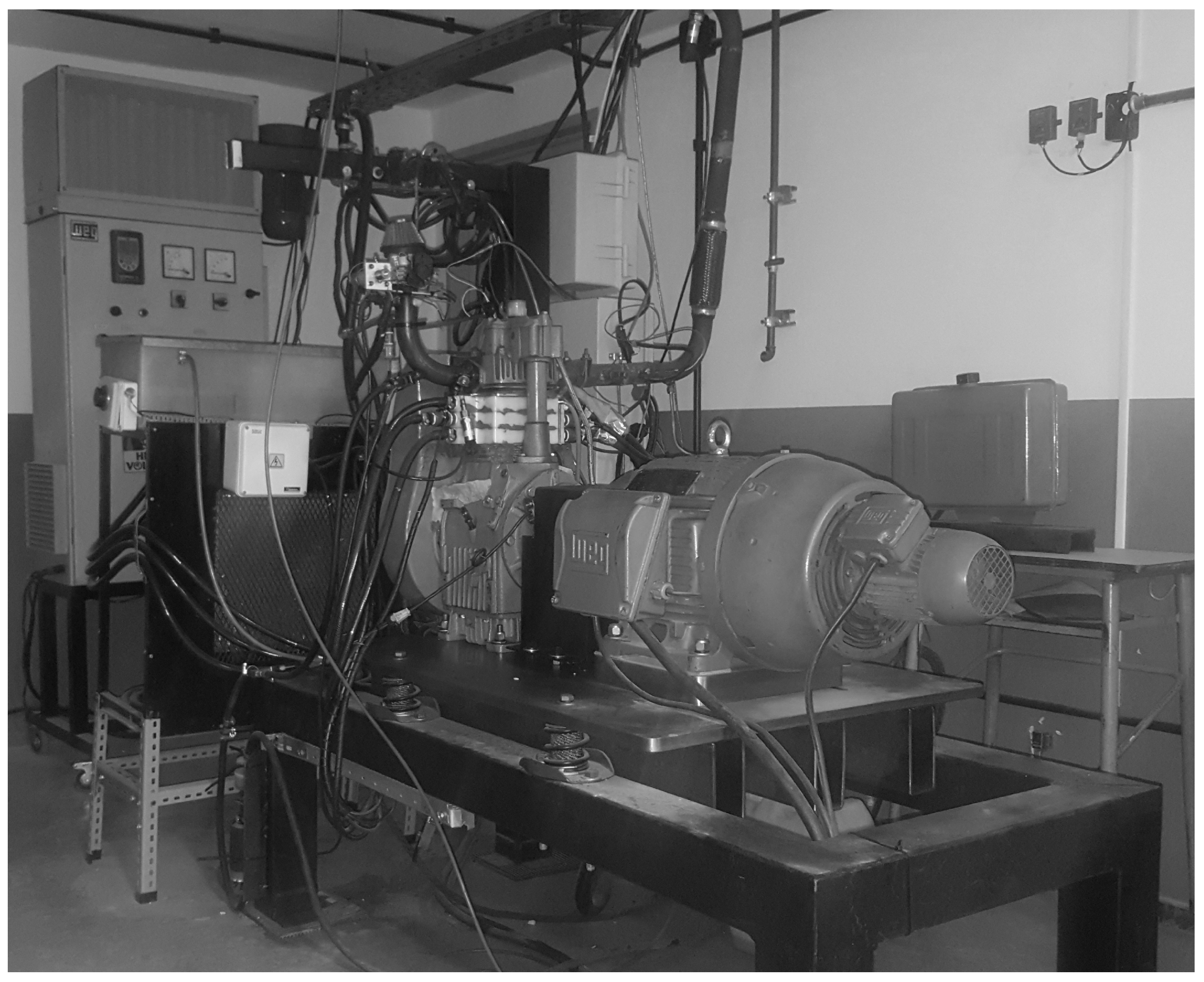
2.1. Engine and Dynamometer
The engine test bench is shown in
Figure 1. The engine is connected to a WEG W22 brake motor that is controlled by a CFW-11 frequency converter control system [
35]. This system allows the remote operation of the ICE under either constant or transient operating conditions in both motored or firing mode.
The experiments were conducted on a single-cylinder Iralvil RV 650 engine with natural aspiration [
36]. The engine was originally conceived and manufactured as a diesel engine. However, it has been reconverted into a spark-ignition engine for research purposes. To do this, several modifications were performed to the engine components and fuel injection system. First, the pistons were changed from the original in-bowl to flat head pistons. This deliberately resulted in the reduction of the engine compression ratio from 17:1 to 10:1. Furthermore, the original engine inlet port was replaced to fit a throttle valve, a gasoline port fuel injector, and several sensors and actuators, which will be described in the following sections.
Table 1 lists the main parameters of the modified engine.
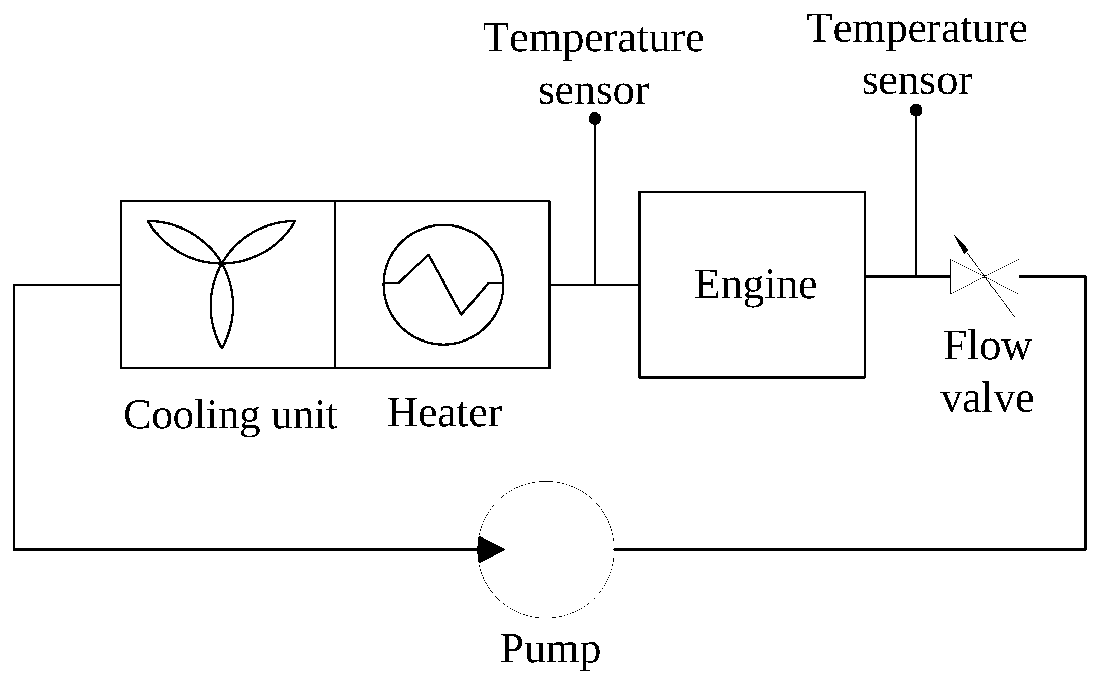
The diesel injection system was removed and replaced by a spark plug and a MicroSquirt V3 gasoline electronic port fuel injection system equipped with a wideband lambda controller. Given that the work at hand is confined only to the gas exchange process of a cold engine, further details on the fuel delivery system are not considered relevant. To have a better control and measurement of the engine temperature and heat fluxes, the original engine air-cooling system was replaced by a closed water-jacket circuit. As shown in
Figure 2, it consists of a water pump, a flow valve, temperature sensors, a
kW electrical heater, and a cooling unit.
Temperature is measured at the inlet and outlet of the water jacket using resistance temperature detectors (, ). The inlet coolant temperature is monitored by a NOVUS N321 controller, which compares the measured temperature to a pre-set reference value. The system consequently enables or disables the cooling unit or the heater to maintain the coolant inlet engine temperature within the pre-set values. The pump operates continuously, with the flow being regulated by an actuated valve. Because the engine is motored, the heat losses in the engine cylinder are relatively small. If a sufficiently large flow of water circulates through the cylinder liner, the temperature change across the latter will be negligible. Thus, the cooling system temperature can be assumed to be constant. Furthermore, as the flow through the jacket is increased, the convection coefficient between the coolant and the cylinder outer wall is augmented, making the thermal resistance at the coolant-cylinder wall boundary negligible compared to that of the in-cylinder gas and the combustion chamber wall. This means that the cylinder wall temperature can be assumed equal to the coolant temperature, thus establishing a precise and steady temperature boundary condition for the simulation models.
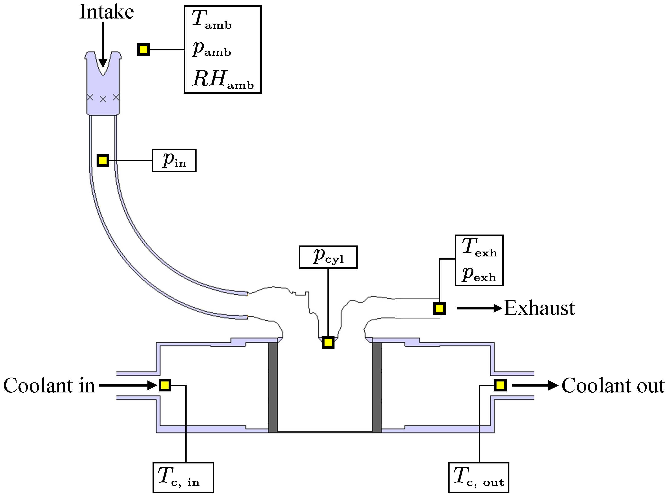
2.2. Sensors and Data Acquisition System
The layout of the engine and the used sensors is shown in
Figure 3, and their characteristics are detailed in
Table 2.
The in-cylinder pressure (
) is measured with a Kistler 6052C piezoelectric transducer, installed on the cylinder head. The sensor signal is conditioned by a Kistler 5011B charge amplifier. The pressure transducer drift is corrected using the manifold air pressure pegging method [
37,
38]. Instantaneous pressures at the intake and exhaust manifolds (
,
) are measured with industrial-type ADZ Nagano pressure transducers. The data generated by the different pressure transducers are recorded every
crank angle degree using a 16-bit National Instruments 6361 data acquisition card. Crankshaft position is measured by a high resolution encoder directly connected to the engine crankshaft, which enables acquiring 2880 data points per cycle. The encoder also provides a single pulse every 360 degrees, referenced to the piston top dead center (TDC) position. This allows synchronizing the acquired data to the instantaneous volume of the engine combustion chamber. This procedure is done by a proprietary software developed at the University of Melbourne [
39]. The exhaust gas temperature (
) is measured with a K-type thermocouple conditioned by an Innovate TC-4 thermocouple amplifier. In contrast, as noted above, the engine coolant temperatures are measured using resistance temperature detectors. Due to the slow response time of the latter compared to the engine temperature dynamics, coolant temperatures are not sampled with crank-angle resolution, but as a steady-state value measurement. Ambient pressure, temperature, and relative humidity conditions (
,
,
) are measured using a Luft WS1200TH weather station.
2.3. Scanning of Engine Internal Geometry
The engine geometry was scanned and digitized using different techniques for each component. Taking advantage of their axial symmetry, the intake and exhaust valves profiles were measured using a profile projector. To scan the inner surface of the intake and exhaust ducts lodges in the cylinder head, silicon molds were made. The molds were then scanned with a Faro Edge arm (precision of
mm [
40]) to produce a cloud of points, which were post-processed using the GeoMagic software and turned into computer models.
Two simplifications were made to obtain the complete geometry of the system. First, given that the exhaust of the engine is connected to the exhaust duct of the engine test cell, which is 20 m long, the computational domain of the exhaust pipe was trimmed to m. Second, given that pressure losses induced by the engine air filter were measured in a SuperFlow 600E flowbench and showed to have no significant impact on the mean volumetric air flow of the engine, the filter was not included in the computational model of the engine.
3. Computational Methodology
The work at hand undertakes the simulation and experimental validation of the full cycle of a cold flow engine, operating under steady state conditions at 1500 rpm. Two cases are defined, varying the position of the throttle valve. In this context, a relative closed position is defined at 35 degrees in contrast to a relative open position where the valve is fixed at 80 degrees. Throughout this section, the computational methods are presented and explained. First, a description of the numerical model employed to solve the governing equations is presented. Subsequently, an explanation is given on how the pseudo-supermesh interface is used in combination with the layering technique to model the moving domains of the engine, Finally, the modeling of the valve events is presented.
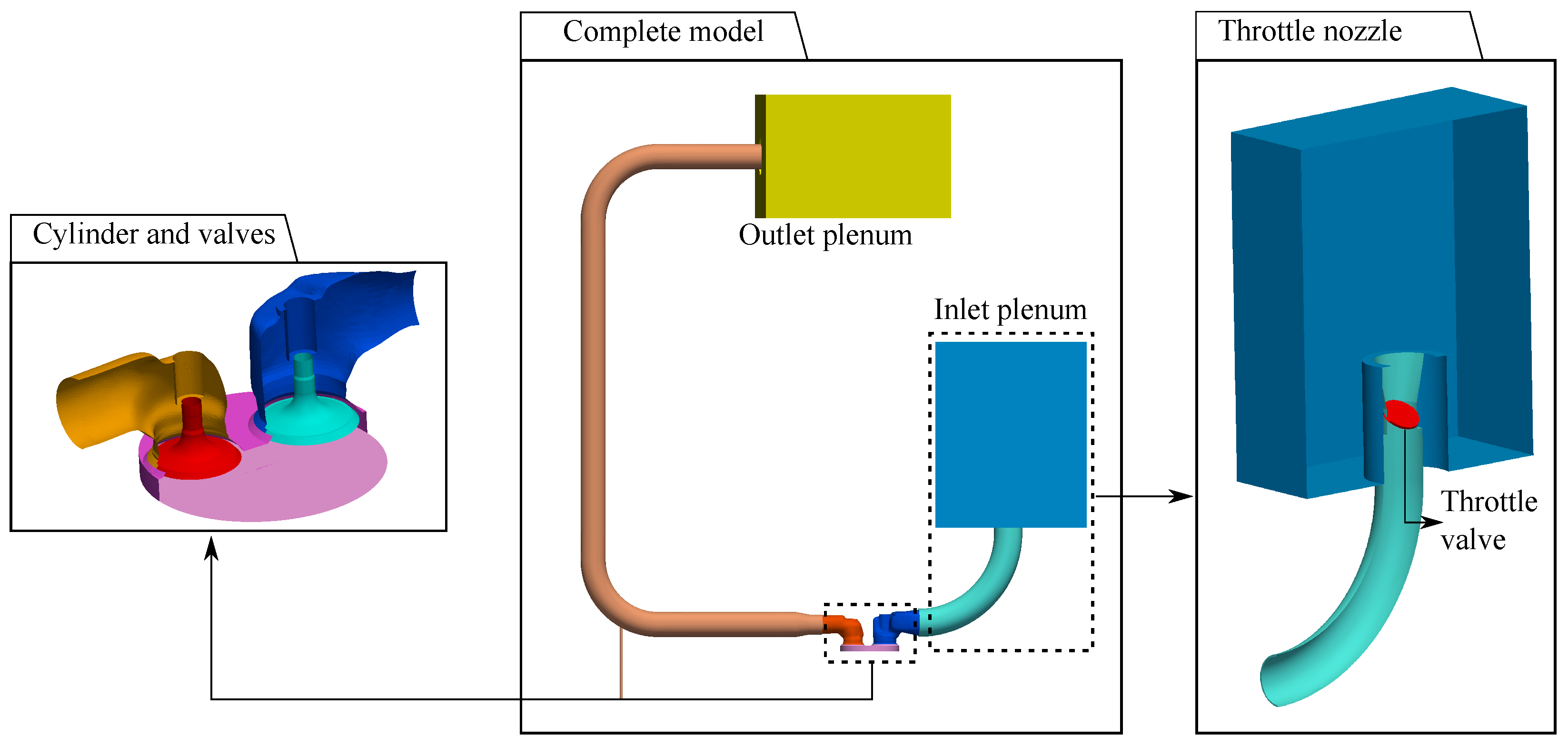
3.1. Computational Domain
As shown in
Figure 4, the boundaries of the thermodynamic system under evaluation are: the throttle valve body, the intake air duct, the cylinder head, the cylinder sleeve, the piston crown, and the exhaust duct. Plenums are added at the beginning and at the end of the inlet and exhaust ducts, respectively, to better represent the impact of the surroundings on the engine flow.
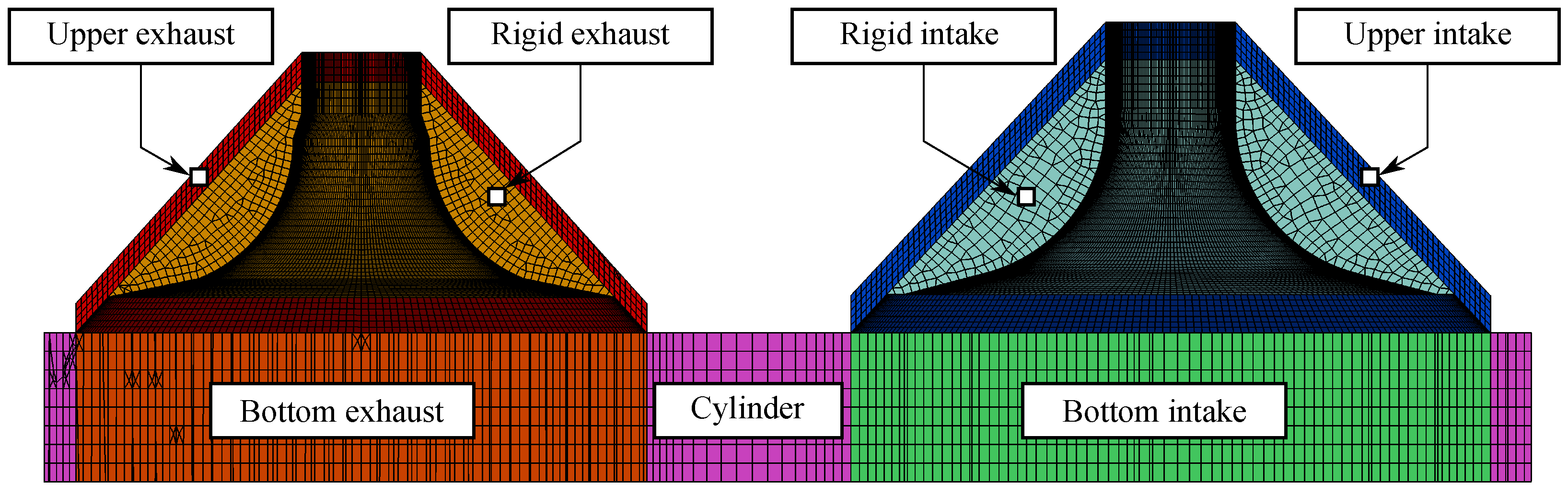
Furthermore, whereas the intake and exhaust ports are of constant volume, other regions have variable geometries to which the applied mesh needs to adapt. These are depicted in
Figure 5 and include the cylinder region and the bottom and upper regions of the inlet and exhaust valves, respectively.
Given the linear motion of the different engine parts, the variable volume of the different domains can be simulated using dynamic extrusion meshes while linking them via a numerical coupling, such as a surface interface. This allows for each region to be managed individually.
As shown in
Figure 5, the cylinder domain is composed of three layering regions called cylinder, bottom exhaust, and bottom intake. Similarly, the layering regions above the valves, which are disposed parallel to the valve seats, define the upper exhaust and upper intake regions. The regions between the layering zones and the valves walls, which move rigidly with the valve body, are named rigid exhaust and rigid intake.
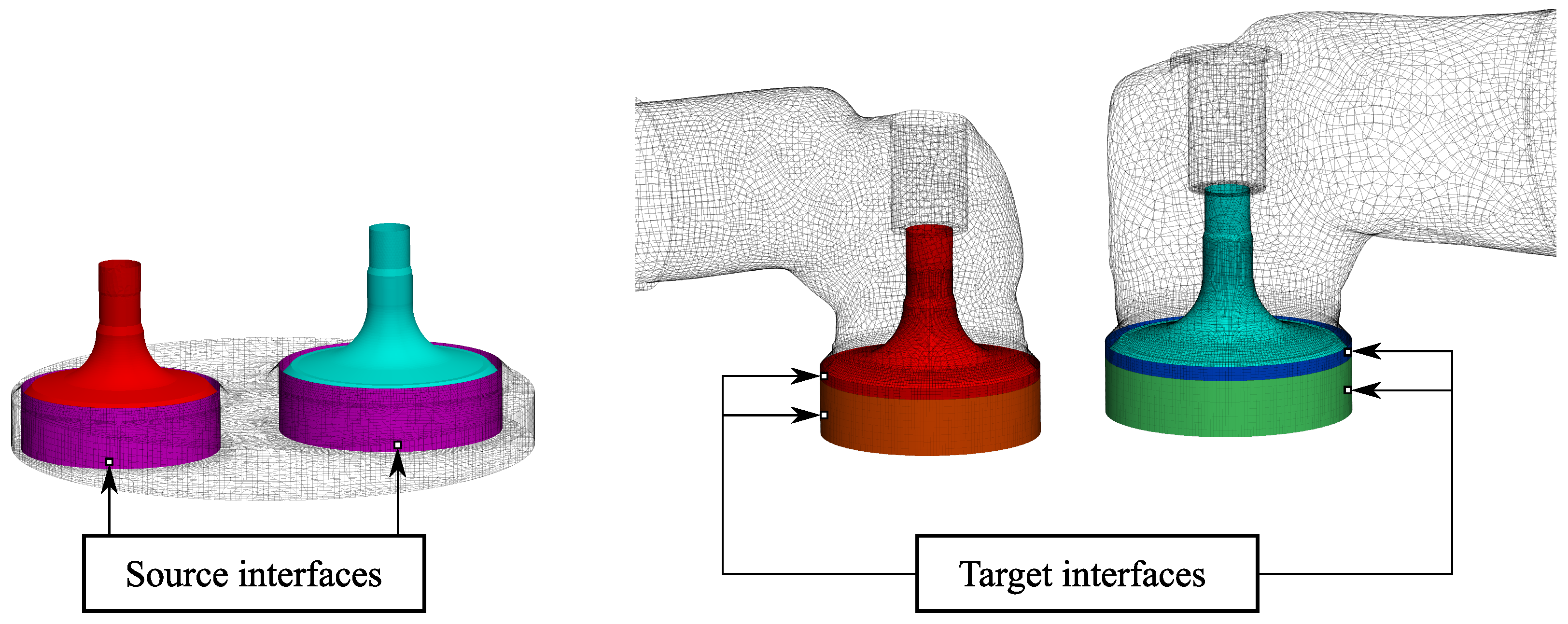
Figure 6 shows the four interfaces between the different domains. These correspond to the upper and lower surfaces of each valve. The lower interfaces link the cylinder to the two regions located below the valves. Analogously, the upper interfaces communicate the upper region of the valves with the cylinder at the zone corresponding to the valve seat.
3.2. Numerical Model
In the next paragraphs, the numerical model is described. Its governing equations, the numerical schemes employed, the boundary and initial conditions applied, and others relevant parameters required to reproduce the simulations are described.
3.2.1. Governing Equations
The governing equations that model the flow are the balances of momentum, mass, energy, and the equation of state for air considered as an ideal gas. The balances are solved with an Arbitrary Lagrangian Eulerian (ALE) strategy where the physical quantities are integrated over a deforming control volume
with moving boundaries
[
41]. Variables are averaged where the Reynolds stress tensor is modelled assuming the Boussinesq hypothesis. In this context, the balance of momentum for a control volume
is
where
is the Reynolds averaged density,
is the Favre averaged velocity,
is the boundary relative velocity,
is the identity tensor, and
p is the Reynolds averaged pressure. The effective viscosity turbulence
is computed as follows:
where
is the molecular viscosity, which is modeled based on Sutherland’s law [
42] using standard values for air, and
is the eddy viscosity computed as
with the parameter
, the turbulence kinetic energy
k, and the turbulence dissipation rate
defined by means of the realizable
model [
43]. The velocity
is computed as
where
is the velocity of the boundary
. The mass balance is solved as
and the total energy balance is solved in terms of the Favre averaged enthalpy
h and the kinetic energy
K as presented as follows:
with Pr
being the effective Prandtl number for air, which is assumed here constant and equal to 0.85. The kinetic energy is computed as
Finally, the equation of state for air as ideal gas is
where R is the ideal gas constant for air and
T is the Favre averaged temperature computed as
where
is the specific heat at constant pressure computed with the Janaf tables [
44] and
is a reference enthalpy for the temperature
.
3.2.2. Discretization and Numerical Setup
The computational implementation required for the resolution of the governing equations is based on the OpenFOAM(R) solver rhoPimpleFoam.This solver is pressure-based where the coupling between the balance equations is achieved using the PIMPLE algorithm, which combines in two nested loops the SIMPLE and PISO algorithms [
45].
Regarding the discretization of the convective and diffusive terms of the balance equations, they are approximated with second-order schemes, and the temporal derivatives are integrated using a second-order backward Euler scheme. The time-step size used is equal to CAD, for which simulations reach a maximum Courant number of approximately 300. For each time-step, seven PIMPLE iterations are employed to iterate the non-linearity of the convective flow. Each simulation is run to get the convergence in engine cycles for the output variables. According to the results obtained, four cycles (eight revolutions of the crankshaft) were enough to reach such a convergence.
3.2.3. Boundary and Initial Conditions
The inlet and outlet boundaries of the engine are configured with the atmospheric conditions measured in the engine room considering a low turbulence intensity. At the walls, a non-slip condition is defined for the velocity, and standard wall-functions are considered for the turbulence variables. On the cylinder, cylinder head, and piston crown, wall temperatures are imposed and set to be equal to the cooling fluid temperature [
46]. The walls at the inlet and outlet ports are configured with the atmospheric temperature.
In regard to the initial conditions, they are defined differently for the cylinder region and the inlet and outlet port regions. The simulation starts with the piston in the TDC position. In this sense, the pressure on the cylinder is set according to experimental measurements, and the temperature is defined assuming an adiabatic transformation from the atmospheric conditions to the TDC conditions. In contrast, the pressure and temperature of the intake and exhaust ports are initialized equal to ambient conditions. At the start of the simulation, the flow is assumed to be stagnant across the entire model assuming low intensity turbulence for the entire domain. It is important to clarify that an optimal setup of the initial conditions is necessary to reduce the simulation time (number of simulated cycles) required to achieve the convergence of the output values in the whole engine cycle. However, initial conditions do not have an impact on the final results, as they are mainly determined by the engine operation parameters and the atmospheric conditions.
The complete set of boundary and initial conditions for all variables are presented in
Table 3 where the numerical condition column presents the keywords employed in OpenFOAM(R) when defining the boundary conditions. More details on them can be found in [
47].
3.3. Valve Events Modeling
In this section, an enhancement performed over the standard pseudo-supermeshes to handle valve events is presented and explained. In a real engine, the valve closure is achieved by the contact between the valve and its seat. Although this is a very simple requirement from a mechanical point of view, its computational simulation involves the elimination of a portion of the mesh located between the valve and its seat, which in turn demands a sophisticated dynamic mesh model. It must be capable of removing or adding boundaries at the closing or opening valve events, respectively. Moreover, when the valve gap approaches zero, the cells would have a high aspect ratio, which may produce numerical problems [
48].
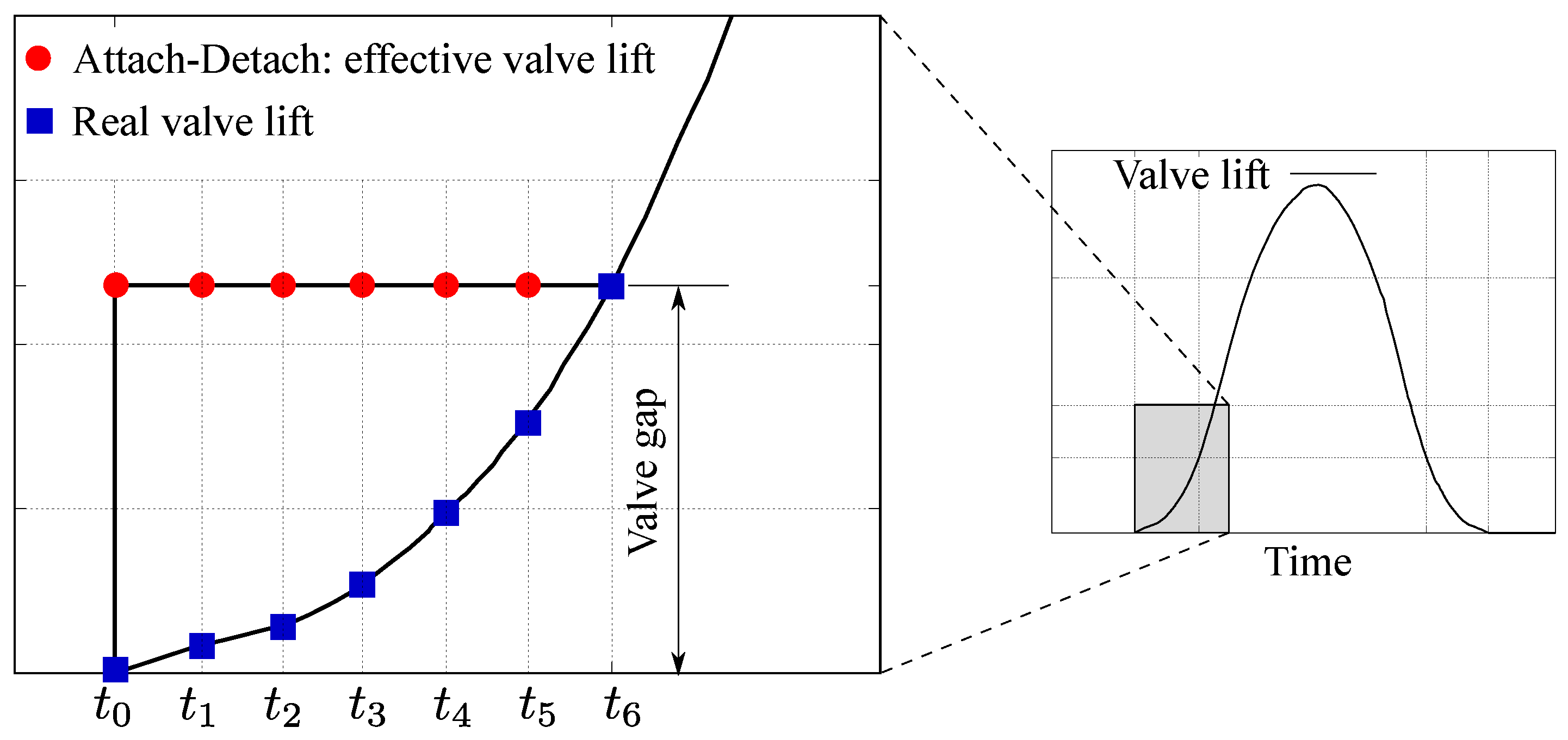
An approach to avoid these numerical issues is the aforementioned “attach-detach” technique. This method links the inner cylinder region to the exhaust and intake ports via a surface interface that can be activated or deactivated. An explanation of this technique in its standard implementation is given in
Figure 7, which describes a valve opening event starting at
. Thus, as the interface is activated early, during the interval
, the effective flow area is larger than the real valve curtain area, resulting in an overestimation of the flow. If the interface would be activated at
, when the minimum mesh gap is equal to the real valve lift, the flow dynamics will be still different to those of the real engine because the opening event will be delayed. Therefore, to minimize flow distortions through the valves, the connection and disconnection technique requires a calibration of the activation time of the interface between both extreme situations.
To overcome these problems, a novel strategy based on a “dual-boundary” approach [
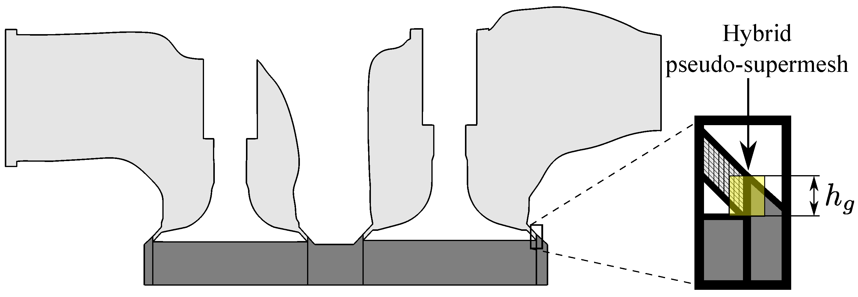
33] is presented. The “dual-boundary” concept refers to the virtual duplication of a surface boundary. This allows setting up alternative boundary conditions without the need of removing or adding elements from the mesh. Based on this concept, the interfaces located over the valves are duplicated. A cross section of the latter is shown in
Figure 8, with the cylinder and port regions differentiated by color. The duplicated interface is used to generate a virtual wall, emulating valve closure. This strategy is referenced in this work as hybrid pseudo-supermesh interfaces (HPSI).
Through the use of HPSI, the mesh sector located between the valve and its seat can be kept frozen. When the valves are closed, the distance (valve gap) between the valve and its seat (
) is filled with a few cell layers, and the cylinder and the port regions are separated by the interfaces acting as walls. Thus, in this condition, the duplicate interfaces are uncoupled and the cylinder and port domains are solved separately. Following the nomenclature defined in [
33], the HPSI may be composed of two pair of surface meshes. One pair is defined by
and
for the cylinder region with faces
and
, respectively. The other corresponds to the interfaces located on the intake and exhaust ports,
and
with faces
and
, respectively. The sub-indexes
c and
b refer to the coupled and non-coupled interfaces, respectively.
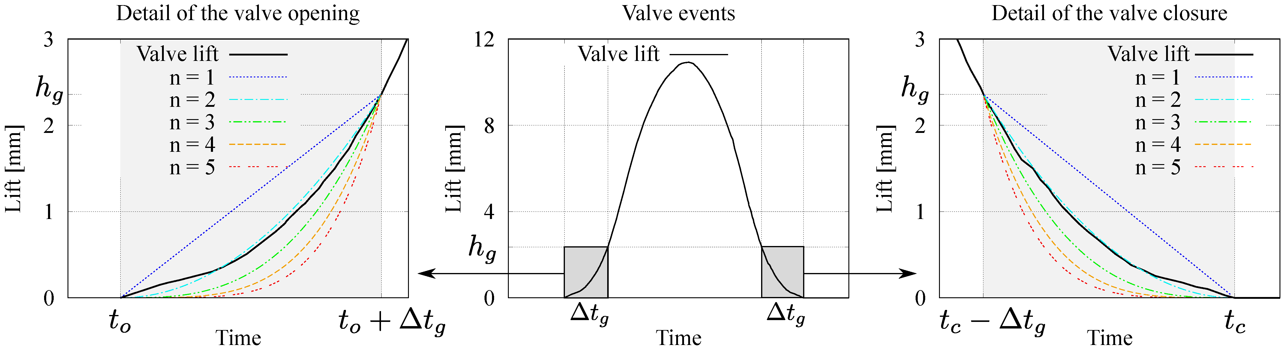
The relative incidence of the coupled and uncoupled interfaces is established by modifying the area of their respective faces based on the position of the valve: open, closed, or in between either. In this way, the pressure drop caused by the real valve lift evolution shown in
Figure 7 can be modeled. The effective area of the valve skirt used for the numerical discretization
can be therefore defined as:
where
is the geometric area of face
K and
is a state function dependent on the valve position. The form of
plays a significant role in the accuracy of the numerical results, as this function models the coupling and decoupling between regions with high pressures and velocity gradients that can introduce numerical discontinuities if the connections are performed suddenly. In the work at hand,
is defined as:
where
n is a model parameter,
is the valve closing time,
is the valve opening time, and
is the time interval required for the valve to reach a lift equal to the mesh valve gap. Therefore, no additional time constants are required for the model.
Figure 9 shows the intake valve lift profile as a function of time and compares it to the profile generated by the function
with different values of
n. For the computational mesh used in this work,
Table 4 details the different time intervals and gap heights for the intake and exhaust valves.
It is important to note that the HPSI area
may be different from the geometric area
A, as the current modeling approach does not consider the pressure losses generated by the shear forces of high velocity flows through small valve gaps. Therefore, it is expected that
would be smaller than
A. Based on this reasoning and in view of
Figure 9, the optimal value of
n for the current engine may be greater than 2.
4. Results and Discussion
Throughout this section, the obtained results are presented and discussed. First, the proposed opening/closing valve model is compared with the attach/detach technique, and their agreement with the experimental results are discussed. Numerical results are then validated against the experimental measurements by comparing several quantitative indicators for engine work, polytropic indexes, and volumetric efficiency. Finally, the computational and parallelization performance of the proposed software is evaluated.
4.1. Experimental Results
Cold engine experimental measurements operating the engine under steady-state conditions at a constant speed of 1500 rpm, and two different angular throttle valve positions, 35° and 80°, are performed. During each test, 300 continuous engine cycles are sampled and recorded. Out of these, a single representative cycle is selected based on the following least squares error (LSE) criterion. The LSE of each individual cycle is calculated as
where the subscripts
i and
j reference the sampling positions throughout each cycle and the cycle number, respectively, and
p is the cylinder pressure. The value of
is evaluated as
The LSE is averaged for every cycle and the one with the least error is selected as the representative cycle of the batch, which in turn is used to assess the simulation results.
4.2. Comparison between the Attach-Detach and HPSI Strategies
A comparison between the attach-detach and the HPSI strategies is performed analyzing the cylinder pressure trace against the experimental data. First, the attach-detach technique is evaluated using three strategies for the interface activation time, and, subsequently, the HPSI strategy is tested using different values of the parameter
n in Equation (
11).
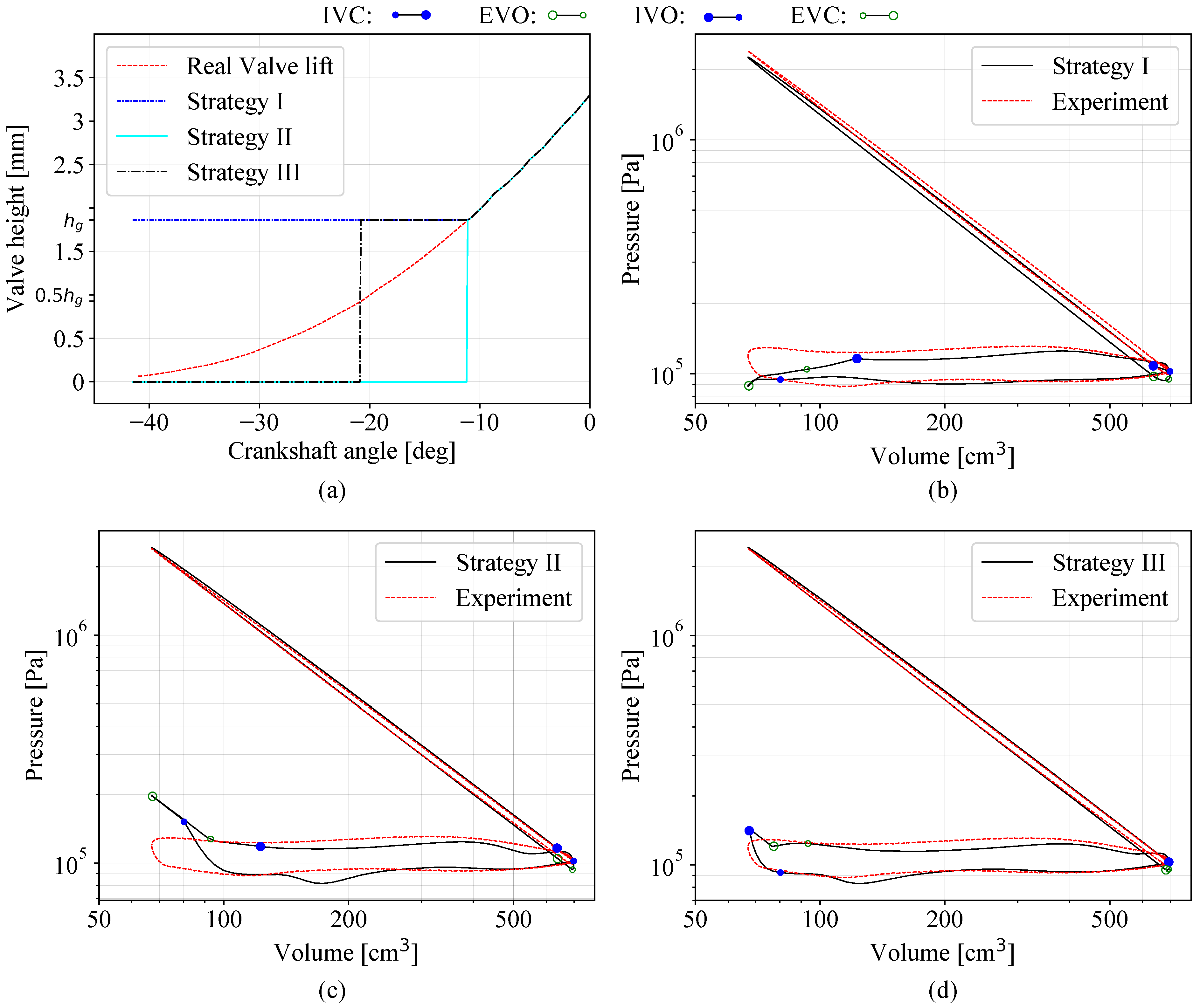
The attach-detach technique is studied using three strategies for the activation time, which are named here as strategies I, II, and III. Using as a reference the times defined in
Figure 7, in strategy I, the valves are opened and closed suddenly at the time
, where the effective valve height during the time interval
is equivalent to the valve gap. In strategy II, the valves are opened and closed at
, which means that the valve height during the time interval
is zero. Finally, in strategy III, the valves are opened and closed when the real valve height is equivalent to half of the valve gap. Here, the numerical valve height between the activation time and
is equal to the valve gap.
The results correspondent to these attach-detach strategies are presented in
Figure 10, where the subfigure (a) schematizes the evolution of the valve height over time for each strategy. The temporal windows of the valve events modeling are indicated by circles as labeled in the upper part of the figure.
From the results, it is concluded that all strategies have drawbacks to adjust the cylinder pressure in the valve overlap region, that is to say, when the two valves are simultaneously opened. In this phase of the engine cycle, the simulation performed with strategy I causes a sudden drop of the cylinder pressure due to an overestimation of the exhaust flow, which is the result of delaying the closing of the exhaust valve. In the opposite case, in strategy II, the cylinder pressure exhibits a spike because the piston is approaching the TDC and the exhaust valve has been closed early. Last, strategy III minimizes the error of the previous strategies, but even it shows a spike because of the anticipated closing of the exhaust valve. Furthermore, the numerical results for the compression and expansion phases are acceptable for strategies II and III, but this is not the case for strategy I, where the peak cylinder pressure is underpredicted. This is because the intake valve remains excessively opened after the BDC and, therefore, a backflow exits towards the inlet depressurizing the cylinder. Another cycle phase where the evaluated attach-detach strategies show an erratic behaviour is the intake one. Here, an abnormal pressure wave is noted that is located at different places in the p-V diagram depending of the strategy applied.
Overall, in view of the results, it is concluded that the attach-detach strategy has issues to adjust accurately all phases of an engine cycle when using meshes with valve gaps in order of those defined in
Table 4. In this situation, a solution could be to decrease the valve gap, but this means significantly increasing the mesh size.
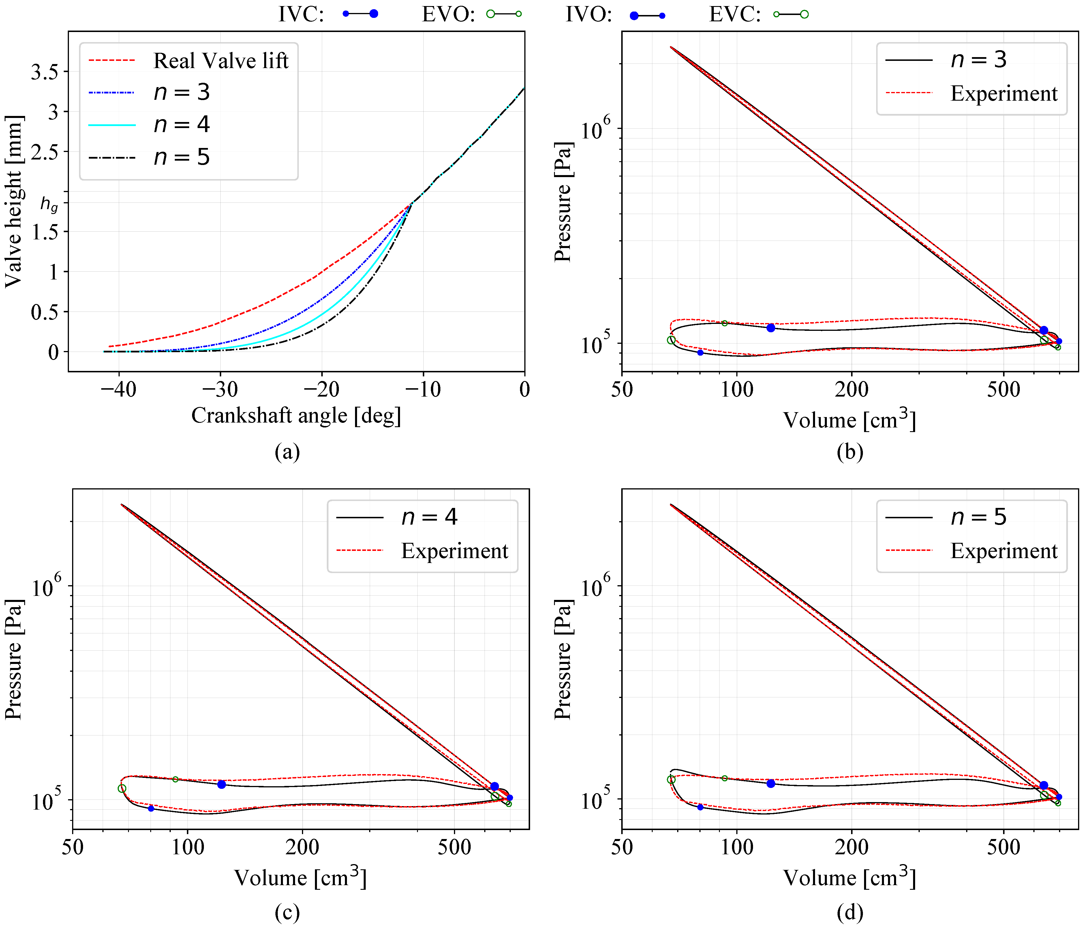
In order to solve the deficiencies of the attach-detach strategy for relatively big valve gaps and without the need of excessive mesh refinement, this work proposes a new strategy using HPSI. As presented in Equation (
10), the current implementation enables defining a parameter
n. A parametric study is carried out for values ranging from
to
, which indicated that the better results are the simulations with
,
, and
. The results of these valve progressions are shown in
Figure 11, including the evolution of the valve height curve for an opening event in subfigure (a).
Contrary to the attach-detach technique results, the HPSI modeling produces pressure traces in the valve overlap region that are smooth for the progressions shown. Likewise, the compression and expansion phases present a very good agreement with the experimental results. Finally, it is highlighted that the intake phase is also well captured, with the results being satisfactory for the three progressions studied. In regard to the influence of the exponent n, its major impact is located in the valve overlap region. The trend of the pressure curves is similar to that observed in the attach-detach technique, where the exhaust valve closing progression defines the peak cylinder pressure in the exhaust phase. In this study, the progression with exhibits the best agreement with the experimental results.
Based on the findings of this study, the HPSI strategy arises as a robust and practical approach to handle meshes with relatively big valve gaps. This is a useful computational tool to take advantage of coarse meshes near the valve gap region in order to achieve whole engine cycle simulations in shorter computational times without impacting the accuracy of the results.
4.3. Validation of the Numerical Model
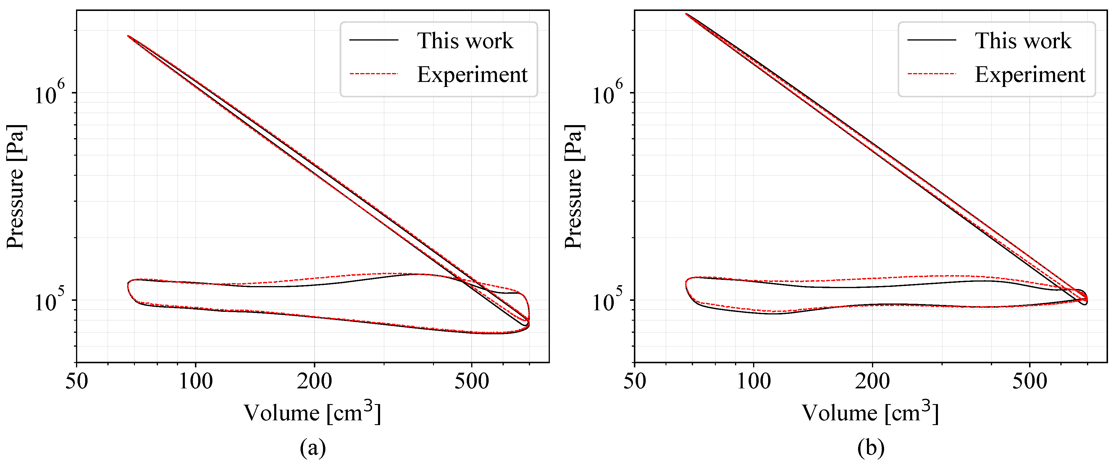
Figure 12 shows the
diagrams of the numerical and experimental representative cycles for both throttle valve positions, 35 and 80 degrees using the HPSI modeling with
. Qualitatively, the results show that the pressure trace generated by the numerical model is in good agreement with the experimental data for both throttle valve positions. In order to make a further analysis of the model accuracy, quantitative indicators are computed and presented in the following paragraphs.
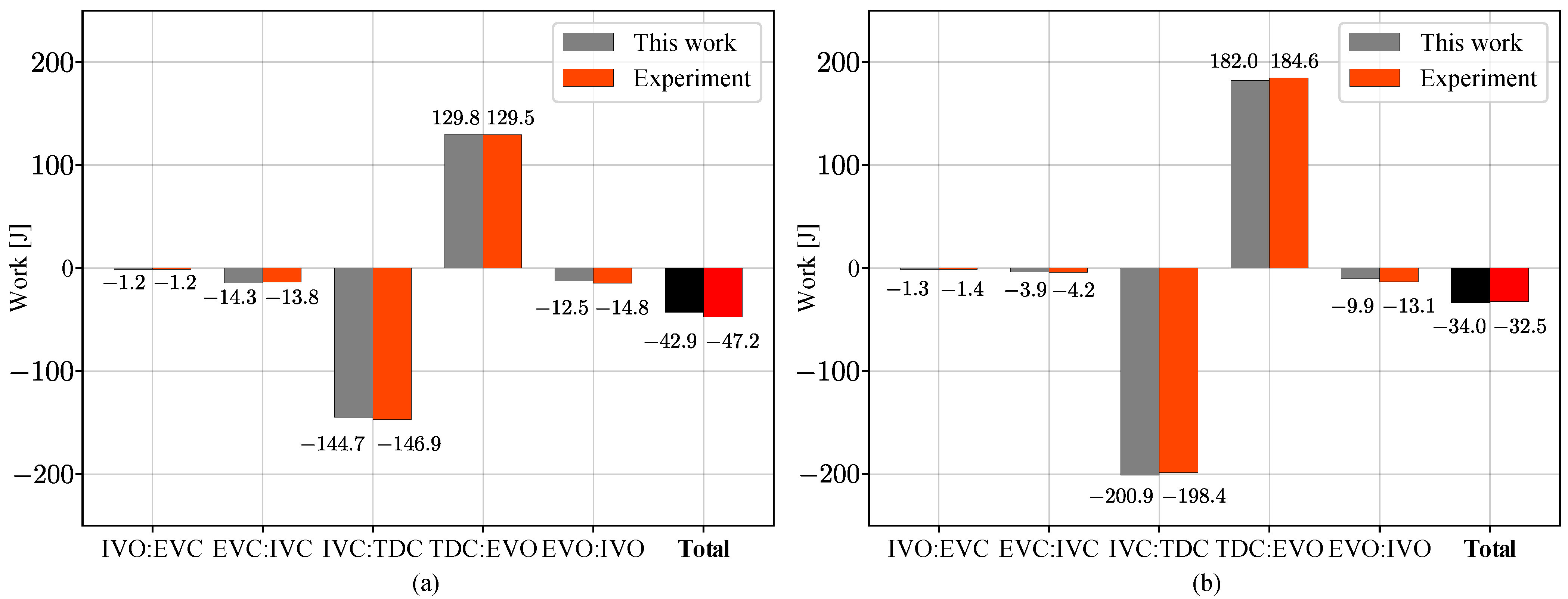
4.3.1. Work by Engine Phases
An useful indicator to analyze the pressure error alongside the whole engine cycle is the total engine work for each phase of the cycle, which is computed as follows:
where
is the average pressure on the piston upper surface minus the pressure in its lower part, which is assumed here as constant and equal to the atmospheric pressure. For the experiment data, the pressure on the piston surface is assumed to be equal to that measured by the pressure transducer. The volumes
and
are the limit volumes for the engine phase being analyzed.
The engine phases considered in this analysis are the compression stroke defined between the IVC and the TDC, the expansion phase defined between the TDC and the EVO, the exhaust stroke defined here between the EVO and IVO, the valve overlap region between IVO and EVC, and, finally, the intake stroke between EVC and IVC.
The total work for each one of the defined engine phases for both tests are presented in
Figure 13 for the throttle positions of 35
and 80
. In light of the results, both numerical simulations have an acceptable prediction for each one of the engine phases computed, which indicates an accurate estimation of the total engine work. Because the engine operates in a motored condition, the total output work is negative, which means that the engine behaves like a compressor consuming energy from the brake motor.
4.3.2. Volumetric Efficiency
The inducted mass is computed using the averaged cylinder pressure at IVC, assuming that the fluid behaves as an ideal gas. As there are no experimental data available for the instantaneous in-cylinder temperature, the numerical results for this value are used instead. With these assumptions, the volumetric efficiency is
where
and
are the ambient temperature and pressure that correspond to the experimental conditions,
p is the numerical or experimental pressure,
is the numerical temperature for both the numerical and experimental volumetric efficiencies,
is the cylinder volume at IVC, and
is the total cylinder volume swept by the piston. The results are listed in
Table 5 and show that the volumetric efficiency predicted by the numerical simulation is very close to that calculated from the experimental measurements.
4.3.3. Polytropic Indexes for the Compression and Expansion Strokes
To further understand the impact of small variations in the fluids properties on the
evolution, separate computations of the polytropic index are performed for the compression and expansion stages of the cycle. In this sense, the
-norm error is minimized to adjust the simulated and measured data to the following expressions:
where
is the mass-weighted average in-cylinder pressure,
V is the cylinder volume, and
and
are constants computed to satisfy the proposed polytropic expressions at IVC during the compression stage and at TDC at the beginning of the expansion stage, respectively; and
and
are the compression and expansion indexes, respectively. The temporal window of Equation (
16) is bounded by the IVC and EVO events, where the piston-cylinder assembly establishes a closed boundary for the thermodynamic system. The value of
is assumed to be constant across the entire cylinder and equal to that measured by the in-cylinder pressure transducer.
Table 6 shows the calculated values of
and
. In line with the good agreement of the compression and expansion phases observed in
Figure 12, the calculated polytropic indexed
and
for the experimental and numerical pressure traces are very similar. Both phases show an averaged
lower than that of the adiabatic evolution (
), indicating heat losses along the process [
49].
Furthermore, the accurate simulation of the intake phase and therefore, the filling of the cylinder in combination with the low error simulation of the compression stroke converges to a good estimation of the cylinder peak pressures. These values are also detailed in
Table 6.
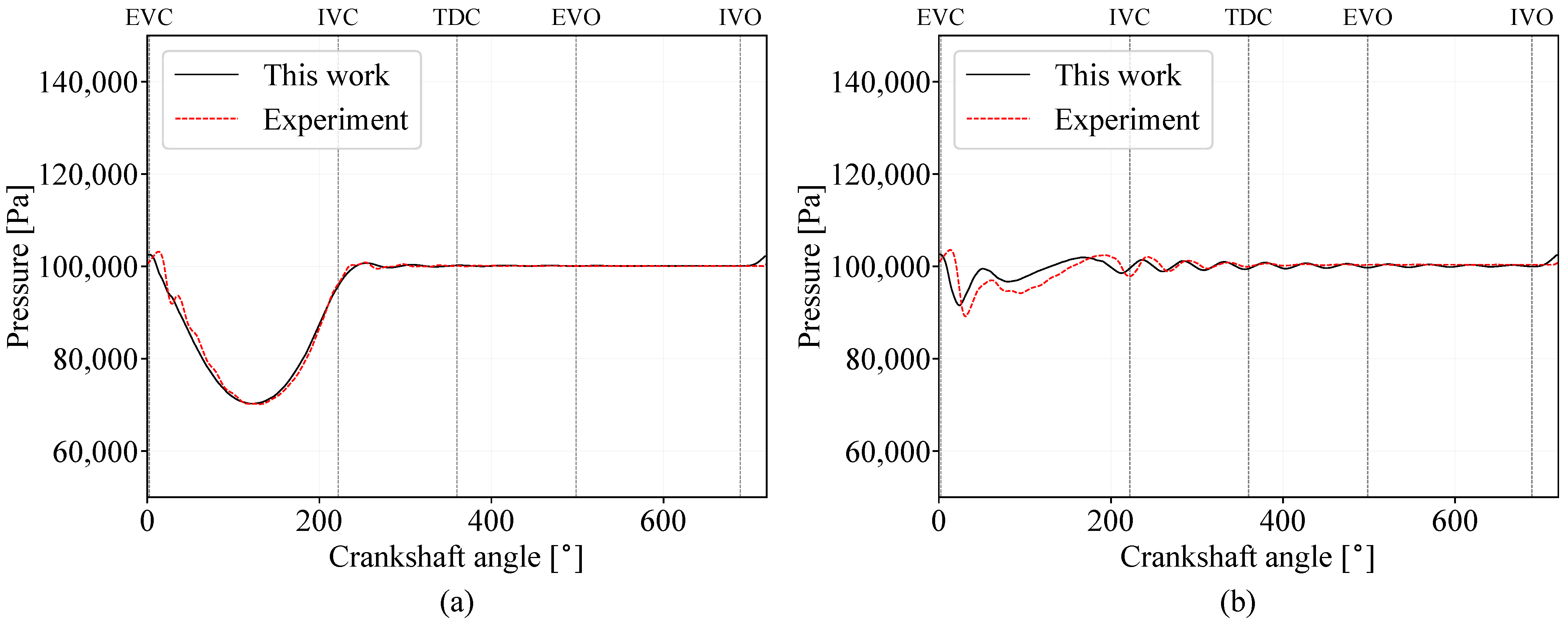
4.3.4. Intake Pressure
The experimental and numeric intake runner pressure are shown in
Figure 14 for both throttle valve positions. Overall, the proposed computational model shows a good agreement with the experimental measurements, which show substantial differences between the two cases. Here, it is important to remark that the intake pressure evolution is not only the result of the flow dynamics through the throttle valve but also through the valves inwards the cylinder where the interface modeling has an important role in order to accurately predict pressure losses. Given the results, the HPSI modeling does not introduce abnormal pressure waves in the intake runner. Moreover, some low amplitude pressure waves after IVC shown in the experimental data are well caught by the simulations.
4.4. Computational Performance
Generally, numerical strategies establish a trade-off between accuracy and computational resources, so when outlining the validity of a given numerical tool it is always important to consider its performance. In this context, this section analyzes the computational performance of the current computational methodology. First, the computational efficiency of the dynamic meshing tool is evaluated by comparing the time required exclusively for the mesh operations with the total simulation time. A scalability test is then performed to assess the parallel performance of the software.
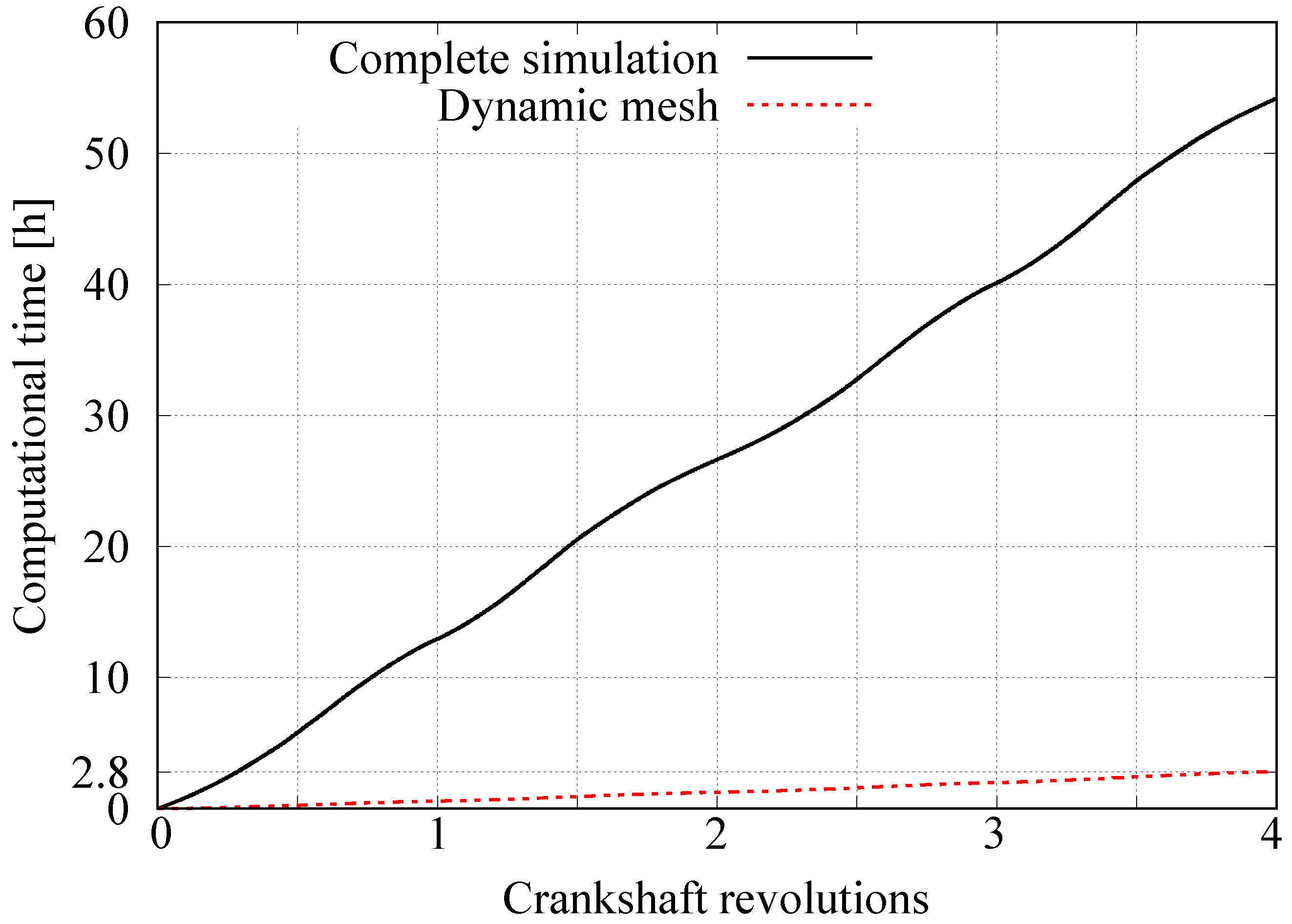
4.4.1. Dynamic Meshing Performance
The efficiency test is run using 60 processors of the cluster detailed in [
50]. The time step size is equal to 0.2 CAD as defined in
Section 3.2.2, and the mesh has approximately
millions of cells.
Figure 15 shows the accumulated computational time required to perform the full engine simulation and the partial accumulated time for the meshing tasks in the same simulation, as a function of the engine crank revolutions. The results show that to complete four engine revolutions, the simulation takes approximately 54 h, whereas the time required to update the mesh is
h. Thus, the current implementation of the dynamic mesh strategy consumes approximately
of the total computational resources.
Based on these results, it is concluded that the proposed dynamic mesh strategy does not produce a significant increment in the total simulation time. Therefore, the good computational efficiency reported in previous work [
30,
33] is replicated here in the context of a four-stroke engine with HPSI interfaces.
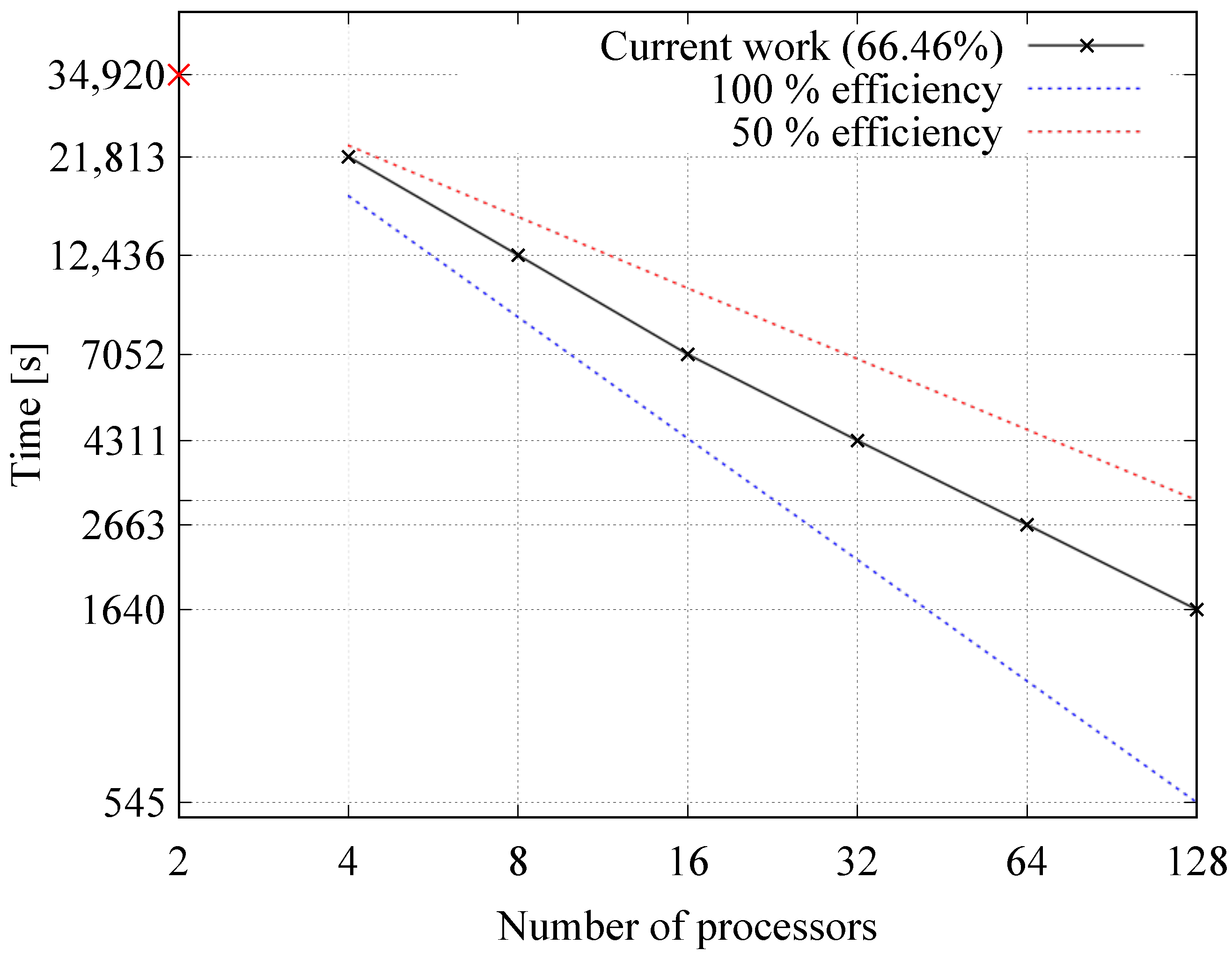
4.4.2. Parallel Performance
To understand the parallelization capability of the proposed dynamic mesh strategy, a strong scalability test is performed. Here, it is taking into account only the dynamic mesh computations without solving the governing equations of the physical problem.
To do this, simulations are performed in parallel using a distributed memory architecture with a Message Passing Interface (MPI) protocol. In this approach, each processor works over a certain portion of the computational domain while verifying that each layering region is decomposed with a two-dimensional partitioning scheme distribution maintained along the extrusion axis [
33]. Attending to this constraint, the current domain is decomposed using 2, 8, 32, and 128 processors.
Figure 16 shows the time required by the solver to perform a whole engine cycle (only mesh operations) as a function of the number of processors used. As a reference, the figure also shows the expected trend for solvers with parallelization efficiencies of
and
. The reference time for the efficiency values is the simulation time elapsed when using two processors, which is the minimum size possible for a parallel run. Results show that the algorithm of the proposed meshing strategy has a parallelization efficiency of around
, meaning that the time needed to perform the required calculations can be considerably reduced by added computational capacity.
5. Conclusions
This paper presented a software tool to simulate four-stroke internal combustion engines. which was implemented in the OpenFOAM(R) framework. For this, the valve events are handled with a new technique, called as HPSI, by using the dual boundary concept. With this strategy, a soft transition between the closed and opened valve states is performed, simplifying the valve gap meshing procedure and increasing the numerical accuracy of the standard attach-detach techniques. The model was validated using experimental data where the main conclusions of the study are presented below:
The standard attach-detach technique generates spikes and abnormal pressure waves in the cylinder for the current mesh employed. In contrast, the HPSI modeling generates smooth and relative accurate cylinder pressure results for different values studied of the parameter n. For the current work, the simulation with exhibited the best prediction of the cylinder pressure in the valve overlap region.
The experimental validation of the numerical model was successful. This observation was supported by several quantitative indicators where the simulation results of these indicators are relatively close to those computed from the experimental data.
The numerical model exhibited a good estimation of the intake pressure dynamics where the sensitivity to the throttle valve position was well captured.
In terms of computational performance, the proposed model showed satisfactory results. The computational time required by the mesh operations was approximately of that required by the whole simulation.
In terms of parallel performance, the current computational implementation showed good prospects for future scalability with its parallelization efficiency close to .
Overall, the presented study showed that the proposed computational tool results in an accurate, reliable, and efficient strategy to simulate the cold flow of a four-stroke engine. The presented tool sets a base towards the development of a full comprehensive four stroke engine computational model. In this sense, future work will be focused on solving turbulent combustion with the liquid injection of a surrogate fuel where the models employed must be implemented to coexist with the current library. In particular, the Lagrangian treatment of the fuel drops must work in conjunction with HPSI to benefit from its computational efficiency.


