High-Order Accurate Numerical Simulation of Supersonic Flow Using RANS and LES Guided by Turbulence Anisotropy

Abstract

This paper discusses accuracy improvements to Reynolds-Averaged Navier–Stokes (RANS) modeling of supersonic flow by assessing a wide range of factors for physics capture. Numerical simulations reveal complex flow behavior resulting from shock and expansion waves and so, a supersonic jet emanating from rectangular nozzle is considered. PIV based experimental data for the jet is available from literature and is used for validation purposes. Effect of various boundary conditions and turbulence modeling approaches is assessed qualitatively and quantitatively. Of particular interest are the inlet conditions considering the turbulence intensity and the effect of upstream air supply duct, the effect of nozzle wall surface roughness on nozzle internal flow and downstream, wall y+ sensitivity for boundary layer resolution and laminar to turbulent transition modeling. In addition to mesh sensitivity, domain dependency is conducted to evaluate the appropriate domain size to capture the kinetic energy dissipation downstream of the nozzle. To further improve the flow characteristics, accounting for the anisotropy of Reynolds stresses is also one of the focuses. Therefore, non-linear eddy viscosity-based two-equation model and Reynolds stress transport model are also investigated. Additionally, the results of baseline linear (Boussinesq) RANS are compared. Corresponding comparisons with high-fidelity LES are presented. Jet self-similar behavior resulting from all simulation fidelities is assessed and it appears that turbulent flow in LES becomes self-similar, but not in RANS. Finally, various factors such as the nozzle geometry and numerical modeling choices influencing the anisotropy in jet turbulence are discussed.

1. Introduction

Computational fluid dynamics has become an important tool in most industrial applications. Modeling turbulent flow accurately is crucial to capture the right physics of the problem. While RANS reduces the computational times, it involves modeling the turbulence transport mechanisms which may lead to some inaccuracies [1]. However, they can be improved by accounting for more physics as close to reality as possible. High Reynolds number flows occur in aerospace application and their simulations guide various engineering processes. The complex shock–boundary layer interactions may lead to boundary layer separation due to adverse pressure gradients and cause instabilities [2,3,4] which makes near-wall region an important topic. While such flows can be better understood using LES, the precursor solution or initial guess starts with RANS. Additionally, for optimization-based studies, a reduced turnaround time is crucial to investigate a complete design space. In such cases, high-fidelity simulations would be impractical considering the demanding computational times. Therefore, obtaining a good quality RANS simulation is beneficial. Several factors combined then capture the right physics. This paper therefore considers various physics-driven boundary conditions, mesh parameters, domain and turbulence modeling-related aspects of CFD such that each present an improvement in itself when compared to a baseline case.

RANS-based investigations of jets and other applications have been conducted previously by many researchers [5,6,7,8,9,10,11,12,13,14]. In some cases, the focus was on assessing the turbulence modeling [5,6,7,8,13] while in other cases a comparison with LES was made [9], while others suggested turbulence models [15]. Other than investigating the turbulence models, accurate boundary conditions are crucial. Effect of inlet modeling, wall modeling, flow non-uniformity, surface roughness, laminar to turbulent transition, mesh and domain dependency are among some of the factors. For example, surface roughness effect on boundary layer flow is important to mimic the actual machined surface geometries. This effect was considered in [16,17,18,19,20]. Liu et al. [19] used surface roughness values in LES of overexpanded jets while Gubonov [20] evaluated nozzles with various surface roughness experimentally. Cresci et al. [21] highlighted the importance of realistic inlet conditions in combustor turbine interface. Bres et al. [22,23] investigated the influence of mesh resolution, inlet conditions, inflow turbulence and wall modeling in LES of supersonic round jets. Some researchers also addressed the effect of incoming turbulence on flow characteristics both experimentally and numerically [24,25]. Hu and Rizzi [26] investigated the transition to turbulence in supersonic and hypersonic nozzles using RANS and highlighted the effect of transition point near throat on the flowfield downstream of the nozzle. In addition to mimicking the boundary conditions correctly, geometry modeling also drives the accuracy of numerical simulations. Smooth and parametric geometry creation is essential in a high-fidelity analysis to capture the curvature accurately as demonstrated by Siddappaji et al. [27,28] for general turbomachinery in compressible and incompressible flow applications. Good meshing practices, geometry creation and domain creation are equally important for accuracy enhancements as highlighted by Siddappaji et al. [29,30].

In most RANS turbulence models, the Reynolds stress tensor is correlated with mean strain rate using a linear relationship which is also known as Boussinesq approximation [1]. Use of Boussinesq RANS and LES has been common for circular jets [31,32,33]. Although Boussinesq approximation is used widely, it imposes some limitations to the accuracy of physics-capture as demonstrated by Schmitt [34] and does not capture the anisotropy of Reynolds stresses. To overcome the assumption of linearity, non-linear relations have been suggested in the literature, for example, the quadratic constitutive relation suggested by Spalart [35]. To directly consider the transport of Reynolds stresses, Reynolds stress models were discussed in [36,37,38]. Applications and evaluations of non-linear RANS and Reynolds stress-based RANS were demonstrated in [39,40,41,42,43,44,45,46,47,48,49]. Yoder [46] investigated various RANS turbulence models including SST, QCR and differential RSM for single-injector cooling flow. Mirjalily et al. [10] calibrated SST model for supersonic flow application. Debonis [13] evaluated the industry standard turbulence models for compression corner; however, non-linear eddy viscosity and Reynolds stress-based models were not considered. Wernet [14] compared jet centerline velocity obtained from RANS with PIV data of supersonic jets. Boychev [49] demonstrated the effect of non-linear RANS in shock wave boundary layer interactions. Authors’ previous work [50,51] has addressed non-linear and Reynolds stress transport-based RANS for supersonic jet.

Apart from investigations at RANS level, some researchers have directly addressed the effect of various boundary conditions at LES level. Among these are the ones reported in [21,22,52,53]. In [52], the effect of inflow turbulence is briefly discussed using various methods, one of them is synthetic eddy method, while Liu et al. [53] presented the effect of adiabatic vs. non-adiabatic nozzle walls on noise using LES. In addition to boundary conditions, numerical dissipation due to the discretization schemes is also important and is discussed in [54] for classical and implicit LES with MUSCL scheme. In [55], effect of mesh resolution in LES is discussed. While these works shed some light on various aspects of accuracy improvements in numerical simulations, they have not yet been demonstrated exhaustively for flow emanating from rectangular nozzle. As shown in authors’ previous work [56], the flowfield is asymmetric on minor and major axis planes and so capturing the anisotropy of turbulence is crucial. Therefore, this work presents improvements in predictions from boundary conditions and turbulence capture point of view, resulting in high-order accurate simulations in this context.

2. Methodology

The nozzle flow is modeled as an ideal gas with standard air. All other parameters considered in RANS are listed in

Table 1. Improvement parameters considered in RANS simulations.

Category	Parameters
Mesh sensitivity	Mesh refinements in nozzle and jet
Domain dependency	Baseline domain, full experimental facility size domain
Inlet modeling	Turbulence intensity Effect of upstream supply duct
Wall modeling	Prism layer sensitivity Isothermal vs. adiabatic walls
Surface roughness	Smooth vs. rough walls
Transition modeling	Gamma transition model
Turbulence capture	Boussinesq (linear) k-omega SST RANS, Quadratic Constitutive relation (non-linear) k-omega SST RANS Linear pressure–strain Reynolds stress model, WALE LES

. Below conditions are presented exhaustively and are categorized as inlet modeling, wall modeling, surface roughness, transition modeling and turbulence modeling. Similar practices are demonstrated by Siddappaji et al. [57]. Capturing important flow physics using grid dependency, domain dependency and best practices in CFD-based analysis of energy transfer enables the designer to dive deep into the transport of momentum, vorticity and energy in the boundary layer and downstream of the device as demonstrated by Siddappaji et al. [58]. Turbulent kinetic energy analysis from control volume approach is shown by [59] in steady RANS.

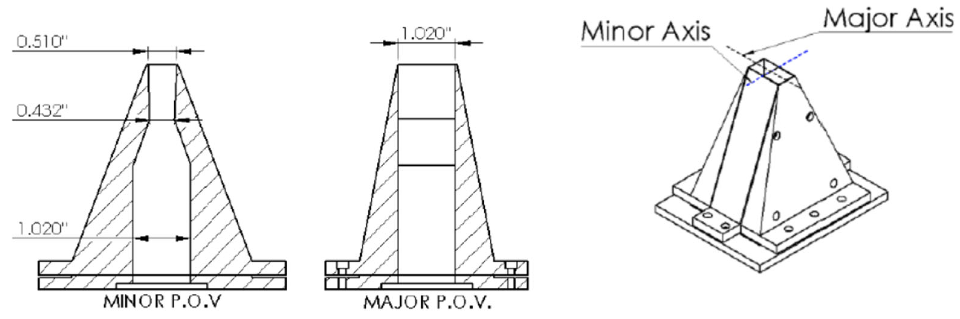
2.1. Nozzle Geometry and Boundary Conditions

Nozzle geometry is shown in Figure 1 and taken from [60]. All simulations correspond to the design pressure ratio of 3.67 and cold flow at inlet temperature of 300 K. They are conducted in Simcenter Star-CCM+ [61]. Figure 1 shows the minor axis and major axis plane of view of the rectangular nozzle geometry along with isometric view. The boundary conditions for nozzle inlet are stagnation pressure, the walls are modeled as no-slip walls and the domain boundaries are freestream at standard atmospheric temperature and pressure. In our previous work [50], the sensitivity of diffusion and dissipation terms in k-omega SST model on jet centerline velocity prediction was addressed by using three variations of blending function. In current work, the lessons learned from previous study are employed for the jet which show benefit of prior analysis. Additionally, the internal flow field resulting from sharp nozzle throat has been analyzed in our previous work [62]. Therefore, for further details on flowfield analysis, readers are pointed towards our previous work [50,62].

2.2. PIV Experimental Data from Literature

Experimental data are reported in [60] and are based on PIV measurements conducted at the University of Cincinnati’s Gas Dynamics Propulsion Lab. The PIV data used for validation purposes is at nozzle pressure ratio 3.67 and at cold flow condition. As explained by Baier et al. [60], the PIV images were taken by seeding the jet flow with 1 μm aluminum oxide particles and ambient seeding was accomplished through olive oil droplet spray. Further details on PIV capability at the University of Cincinnati can be found in [63,64]. Since current work only deals with numerical simulations, details of experimental setup are omitted for the sake of brevity.

2.3. Governing Equations

Governing equations for RANS and LES are listed in this subsection. In RANS, two turbulence models are used as mentioned in Table 1, namely Boussinesq and QCR k-omega SST and Reynolds stress transport model with linear pressure–strain relation. Equations (1) and (2) denote the transport equations for k-omega SST turbulence model [63]. The QCR RANS is based on the relation suggested by Spalart [35].

$$\frac{\partial }{\partial t}\left(\rho k\right)+\mathit{\nabla }.\left(\rho k\overline{v}\right)=\mathit{\nabla }.\left[\left(\mu +{\sigma }_k{\mu }_t\right)\mathit{\nabla }k\right]+P_k-\rho {\beta }^{*}{f}_{{\beta }^{*}}\left(\omega k-{\omega }_0{k}_0\right)+S_k,$$

(1)

$$\frac{\partial }{\partial t}\left(\rho \omega \right)+\nabla .\left(\rho \omega \overline{v}\right)=\mathit{\nabla }.\left[\left(\mu +{\sigma }_{\omega }{\mu }_t\right)\mathit{\nabla }\omega \right]+P_{\omega }-\rho \beta f_{\beta }\left({\omega }^2-{\omega }_0{}^2\right)+S_{\omega }.$$

(2)

In Equation (1), the first term on right hand side is the diffusion term combining turbulence diffusion and molecular diffusion. $P_k$ is the production term. The third term on right hand side represents dissipation and the fourth term is user defined source term.

Equation (3) shows the Reynolds stress transport equation used in Star-CCM+ [61] and, as mentioned previously, it uses linear-pressure strain relation by Gibson and Launder [36].

$$\frac{\partial \left(\rho R\right)}{dt}+\mathit{\nabla }.\left(\rho R\overline{v}\right)=\mathit{\nabla }.D+P+G-\frac{2}{3}I{\gamma }_M+\underset{\_}{\varphi }-\rho \underset{\_}{ϵ}+S_R,$$

(3)

where R is the Reynolds stress tensor, $\rho$ is the density, $\overline{v}$ is the mean velocity, D is the Reynolds stress diffusion, P is the turbulent production, G is the buoyancy production, I is the identity tensor, ${\gamma }_M$ is the dilatation dissipation, $\underset{\_}{\varphi }$ is the pressure–strain tensor, $\underset{\_}{ϵ}$ is the turbulent dissipation rate tensor and $S_R$ is the user-defined source term.

LES filtered governing equations of mass, momentum and energy are given as [61].

$$\frac{\partial \rho }{\partial t}+\mathit{\nabla }.\left(\rho \tilde{v}\right)=0,$$

(4)

$$\frac{\partial \left(\rho \tilde{v}\right)}{\partial t}+\mathit{\nabla }.\left(\rho \tilde{v}⨂\tilde{v}\right)=-\mathit{\nabla }.\tilde{p}I+\mathit{\nabla }.\left(\tilde{T}+T_{SGS}\right)+f_b,$$

(5)

$$\frac{\partial \left(\rho \tilde{E}\right)}{\partial t}+\mathit{\nabla }.\left(\rho \tilde{E}\tilde{v}\right)=-\mathit{\nabla }.\tilde{p}\tilde{v}+\mathit{\nabla }.\left(\tilde{T}+T_{SGS}\right)\tilde{v}-\mathit{\nabla }.\tilde{q}+f_b\tilde{v}.$$

(6)

In the above equations, $\rho$ is the density, $\tilde{v}$ is the filtered velocity, $\tilde{p}$ is the filtered pressure, I is the identity tensor, $\tilde{T}$ is filtered stress tensor, $f_b$ is resultant of body forces, $\tilde{E}$ is filtered energy per unit mass, $\tilde{q}$ is the filtered heat flux. LES uses WALE subgrid-scale model suggested by Ducros [65] and is outlined below.

$${\mu }_t={\left(C_w∆\right)}^2\frac{{({𝓈}_{ij}^d{𝓈}_{ij}^d)}^{\raisebox{1ex}{$3$}\!\left/ \!\raisebox{-1ex}{$2$}\right.}}{{\left(\overline{S_{ij}} \overline{S_{ij}}\right)}^{\raisebox{1ex}{$5$}\!\left/ \!\raisebox{-1ex}{$2$}\right.}{({𝓈}_{ij}^d{𝓈}_{ij}^d)}^{\raisebox{1ex}{$5$}\!\left/ \!\raisebox{-1ex}{$4$}\right.}}.$$

(7)

In the above equation, ${\mu }_t$ is the eddy viscosity, $C_w$ is the model constant and is equal to 0.544, ${𝓈}_{ij}^d$ is the traceless symmetric part of the square of the velocity gradient tensor and $\overline{S_{ij}}$ is the mean strain rate.

2.4. Baseline RANS

The baseline case is obtained by conducting mesh dependency and domain dependency study. Other than that, it does not use any of the improvement parameters listed in Table 1 and so is referred as baseline. The domain size of this case is 100 De downstream, 10 De upstream and 15 De sideways from nozzle exit. The refinement zones include the regions inside the nozzle and within the jet up to 20 De downstream of the exit. The nozzle walls are adiabatic and are smooth, i.e., surface roughness value is not used. To capture the boundary layer, 15 prism layers are used with expansion factor of 1.5 and a total thickness of 1 mm. The convective fluxes are discretized using second-order hybrid upwind and bounded central scheme and uses k-omega SST turbulence model with Boussinesq approximation. In order to first assess this case, a comparison with PIV experimental data is provided. Figure 2 shows the jet centerline velocity. It is overpredicted by CFD compared to experiments which is a result of dissipation and diffusion terms in the governing equations of turbulence model as shown previously by authors [50]. Experimental data from [60] is used to validate the numerical results. CFD results show overprediction in the length of potential core as expected which is the result of low diffusion and dissipation [50]. The goal is thus to improve the physics capture of baseline RANS using several improvement parameters listed in Table 1 and finally compare with LES results.

2.5. Mesh Sensitivity

Before diving deeper into the physics capture aspect, mesh sensitivity and domain dependency study are conducted. The refinement zones in the region internal to nozzle and in the jet are crucial to capture the shocks and expansion waves. Therefore, three grids are assessed. The mesh refinement regions were in the nozzle, jet nearfield and mixing region. Each zone used values listed in

Table 2. Mesh sensitivity parameters for RANS simulations.

Case Abbreviation	Number of Cells (Million)	Refinement Size (m)	Total Pressure at Nozzle Exit (Normalized by Pin)
Coarse	6	De/25	0.965
Medium	8	De/30	0.964
Fine	10	De/35	0.964

. For this study, the number of prism layers were the same since the y+ value was close to 1 and changing the prism layers would have affected the near-wall dynamics.

Figure 3 shows a zoomed-in view of the grid at nozzle exit. Figure 4 shows the jet centerline velocity for the three grids. Since fine mesh RANS is closer to the PIV data in the mixing region, it is used.

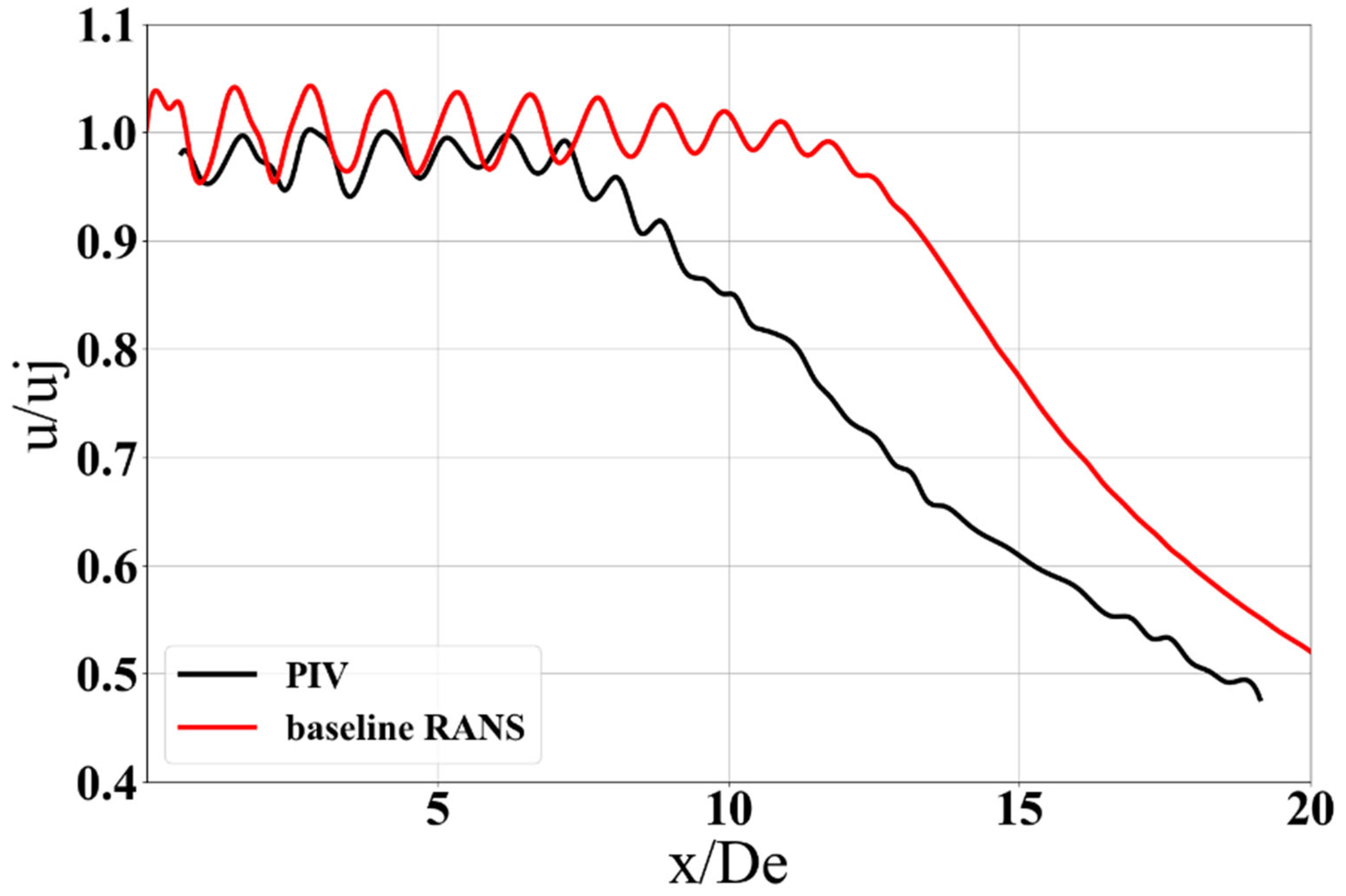
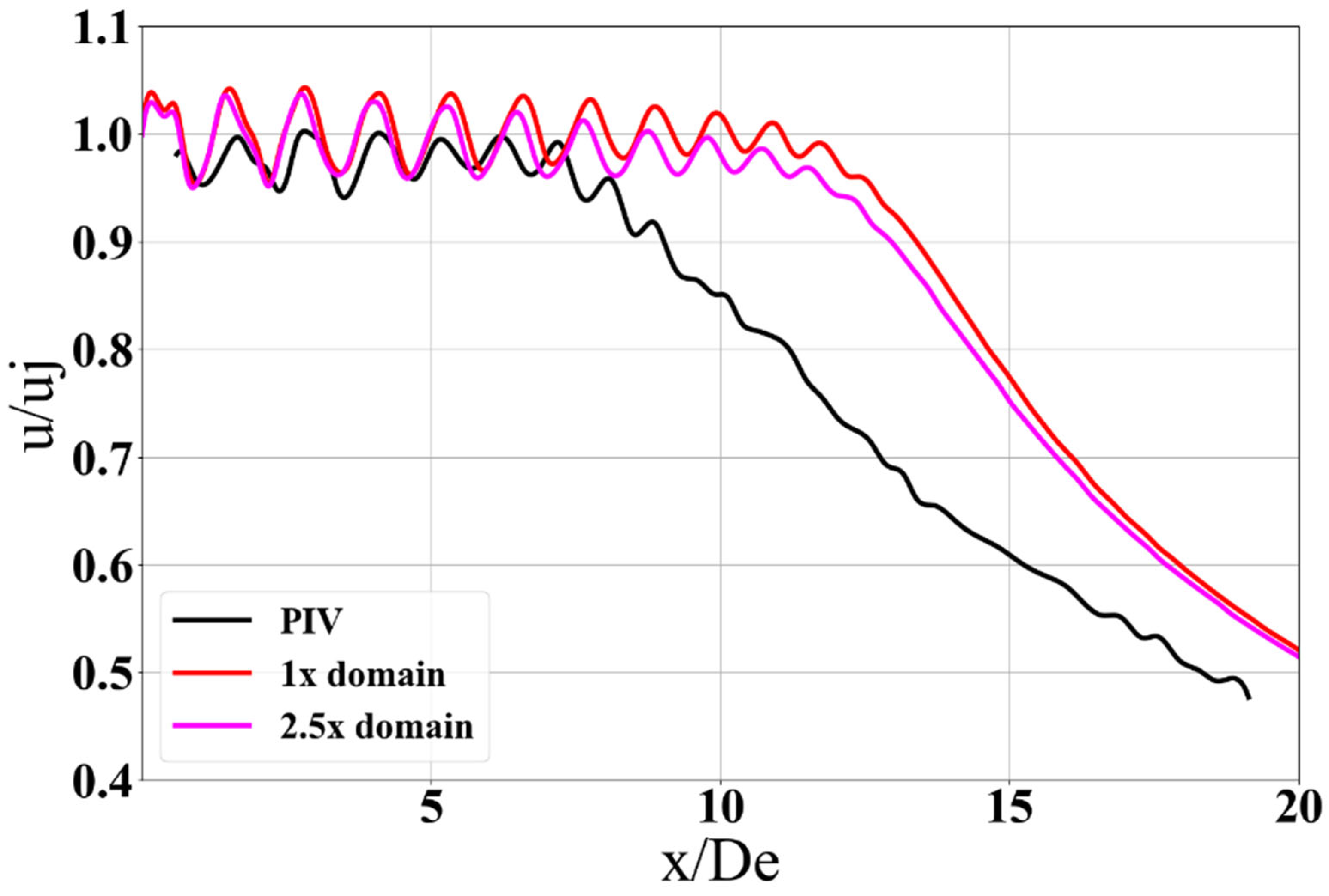
2.6. Effect of CFD Domain Size in RANS Simulations

CFD domain size is one of the important aspects which has an effect due to the placement of the boundary conditions from the area of interest [57]. Free shear layers and jets are sensitive to the freestream boundary in simulation setup. The goal of this sub-section is to evaluate the impact of CFD domain size on the nearfield of rectangular jets. A baseline case with domain size 100 De × 15 De × 10 De is considered which is referred to as 1× domain. The domain in this case is sufficiently downstream of the nozzle exit. From the experimental measurements of Baier et al. [60], the facility where the experiments were conducted has a size of ~2.5 times the current domain size. Therefore, another domain size is considered which is equivalent to the experimental facility size and is referred to as 2.5×. Figure 5 below indicates the jet centerline velocity comparison at 1×, 2.5× domain and with the experimental data. The velocity in the close proximity to the nozzle exit is the same in both cases; however, after x/De > 7, the domain tends to affect the centerline velocity prediction. Interestingly, the peaks reduce in amplitude and the mixing occurs faster than the baseline case. However, domain size effect is within 1–2% of the baseline case. Increasing the domain size increases the computational cost without significant impact. Clearly, 1× domain size is sufficiently wide.

3. Results—Improved Accuracy RANS

This section presents the results of various factors listed in Table 1, except for the mesh sensitivity and domain dependency study as they are discussed previously.

3.1. Inlet Modeling

The nozzle inlet modeling is an important topic because the state of incoming air boundary layer affects the flow dynamics. Various approaches can be taken to account for this effect, for example, by directly considering the upstream supply duct or by using a value of turbulence intensity or by using a velocity/pressure profile to model the inlet. In present work, the upstream air supply duct with a 90-degree bend is modeled.

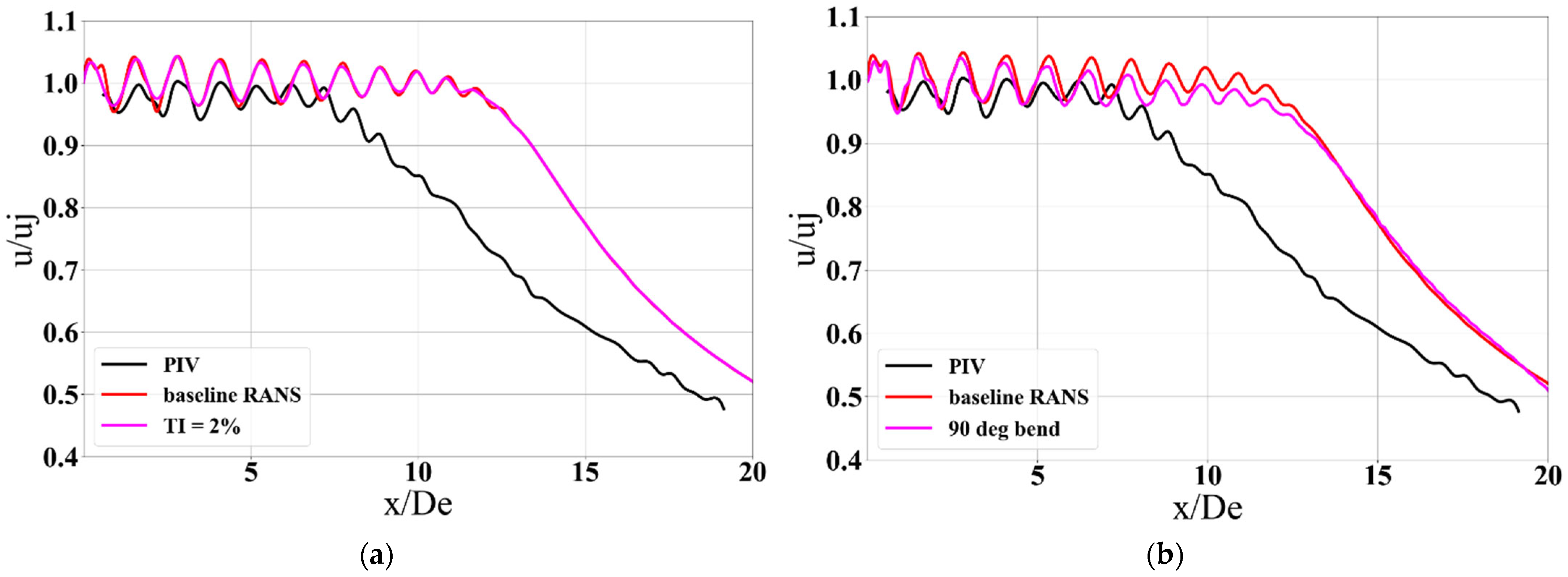
3.1.1. Turbulence Intensity

The incoming compressed air supplied to the nozzle has a level of turbulence present in it which is represented by turbulence intensity. The simulation with 2% turbulence intensity showed negligible effect on the centerline velocity as in Figure 6a.

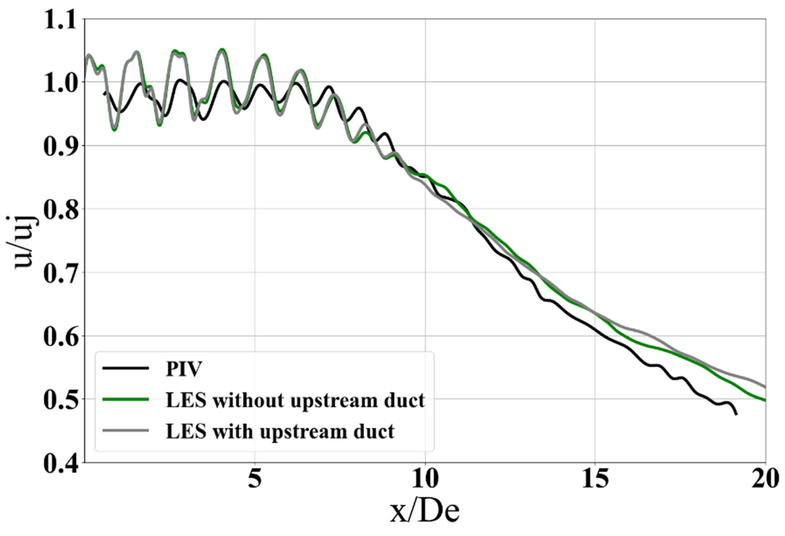
3.1.2. Effect of Upstream Air Supply Duct

Based on the experimental data reported in [60], the supply air to the nozzle inlet is provided through a 90-degree bend. In certain cases, this inlet was modeled as uniform pressure, uniform temperature inlet, while some researchers have used temperature profile at nozzle inlet as reported in [23]. The approach in present work is to directly model the upstream duct. This accounts for the flow turning effects due to the bend. Directly modeling the upstream duct allows the flow to develop as it reaches the nozzle inlet. Figure 6b shows that the case with upstream supply duct has shorter amplitudes of velocity oscillations and mixes out sooner. In addition, the differences in the amplitudes of velocity oscillations are coming from the induced streamwise vorticity on account of upstream air supply duct. This can be clearly seen from Figure 7. However, this does not cause significant differences in the predicted centerline velocities up until x/De = 6 as seen from Figure 6b. Beyond this point, the velocity decays more rapidly than the baseline case.

Figure 7a,b show the streamwise vorticity normalized by De/uj with and without upstream duct cases, respectively. The cross-flow planes are illustrated such that they start at the nozzle inlet and move downstream along the nozzle length. Due to the 90-degree bend, additional vorticity fields are formed at the bottom of nozzle and are responsible for enhanced mixing. This is not seen in the case without the upstream bend.

Modeling the upstream duct affects the jet centerline velocity prediction by ~1–2% and there is a reduction in peak amplitude of the jet centerline velocity. After x/De > 4, the peaks of the case with duct reduce compared to the baseline on account of better mixing due to the generation of streamwise vorticity induced by the upstream duct.

3.2. Wall Modeling

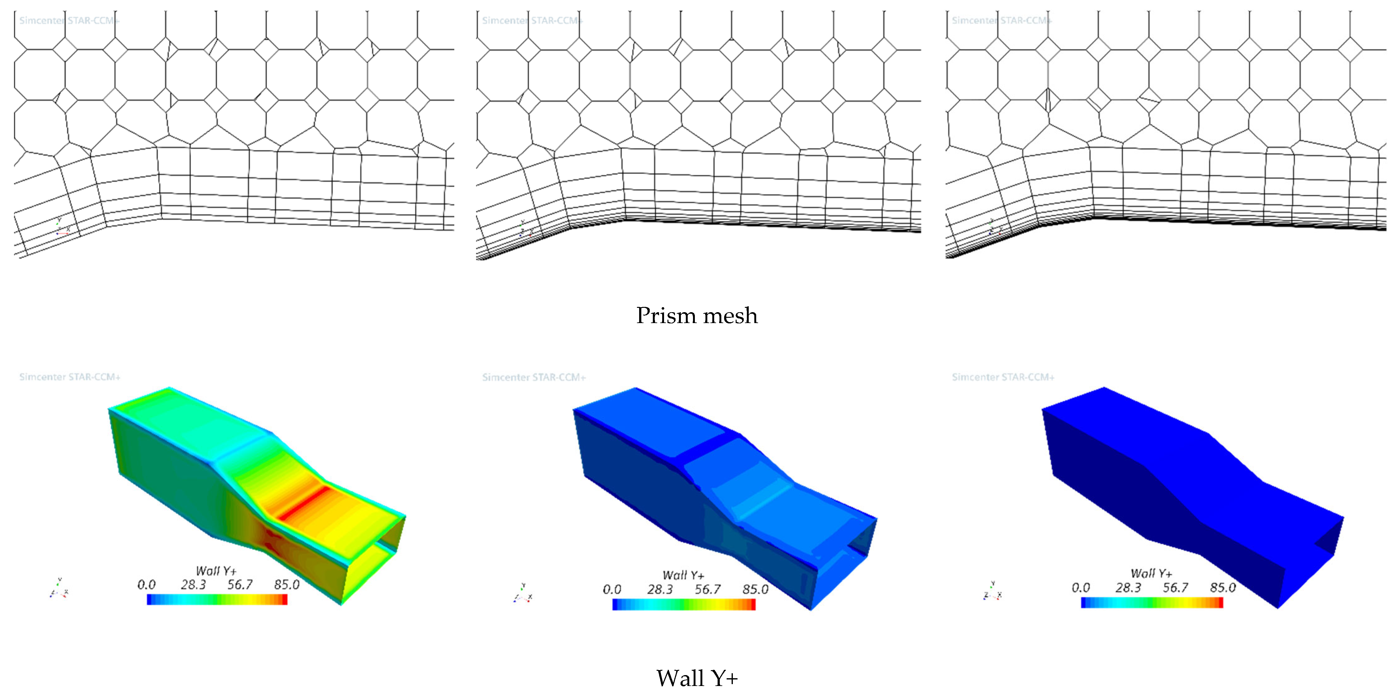
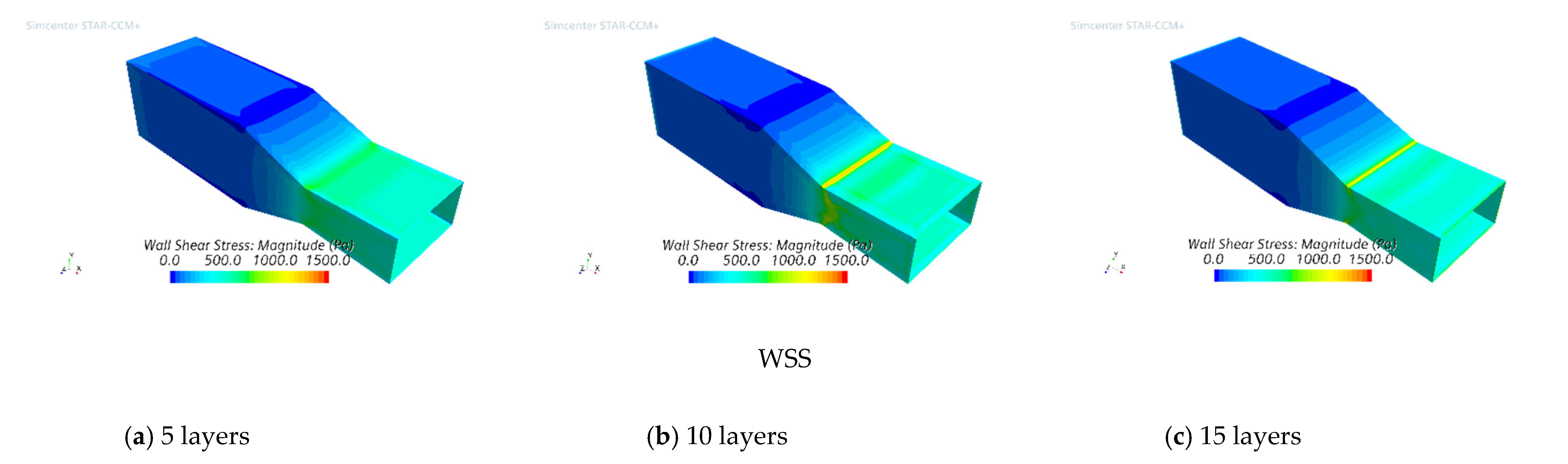
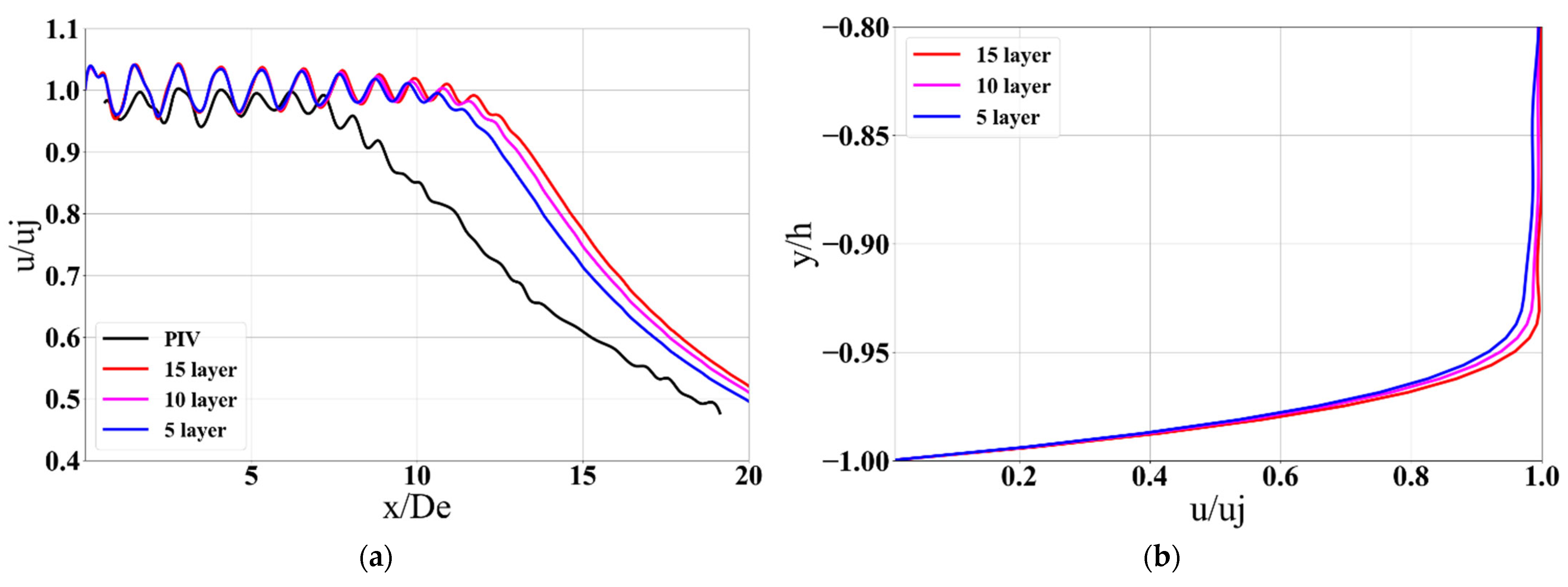
3.2.1. Prism Layer Sensitivity

This section discusses the prism layer sensitivity for internal flow physics. Due to the presence of shock boundary layer interactions in the nozzle [62], it is imperative to evaluate this sensitivity. For such flows, the wall y+ close to 1 is desirable to fully resolve the boundary layer, which increases the number of grid points in the boundary layer and thus the computational time. Figure 8 evaluates three prism layer cases with 5, 10, 15 layers, maintaining the total thickness of 1 mm and by changing the number of layers in the boundary layer mesh. The three cases use 5-, 10- and 15-layer prism mesh. Figure 8 also shows the wall shear stress values and wall y+ values for the three cases. As seen, 5-layer case has greater wall y+ value and 10-layer case has lower wall y+ value. With lower wall y+ values, the wall shear stress magnitudes are lower than the other two cases. This is since the first point in the boundary layer lies outside of viscous sublayer. In 15-layer case, the wall y+ is close to 1 and so the wall shear stress magnitudes are higher as compared to case with 5 layers.

Additionally, Figure 9a,b show the jet centerline velocity comparison and nozzle exit boundary layer profiles for the three cases. The boundary layer thickness is higher for 5-layer case and decreases as the number of layers increase. However, the three boundary layers are turbulent and the case with 5 layers has thicker turbulent boundary layer. This directly affects the jet centerline velocity prediction. For example, the 5-layer case has thicker boundary layer which results in reduced momentum in boundary layer and causes the mixing earlier than 15-layer case. Since 15-layer case results in wall y+ close to 1, it is used for further analysis.

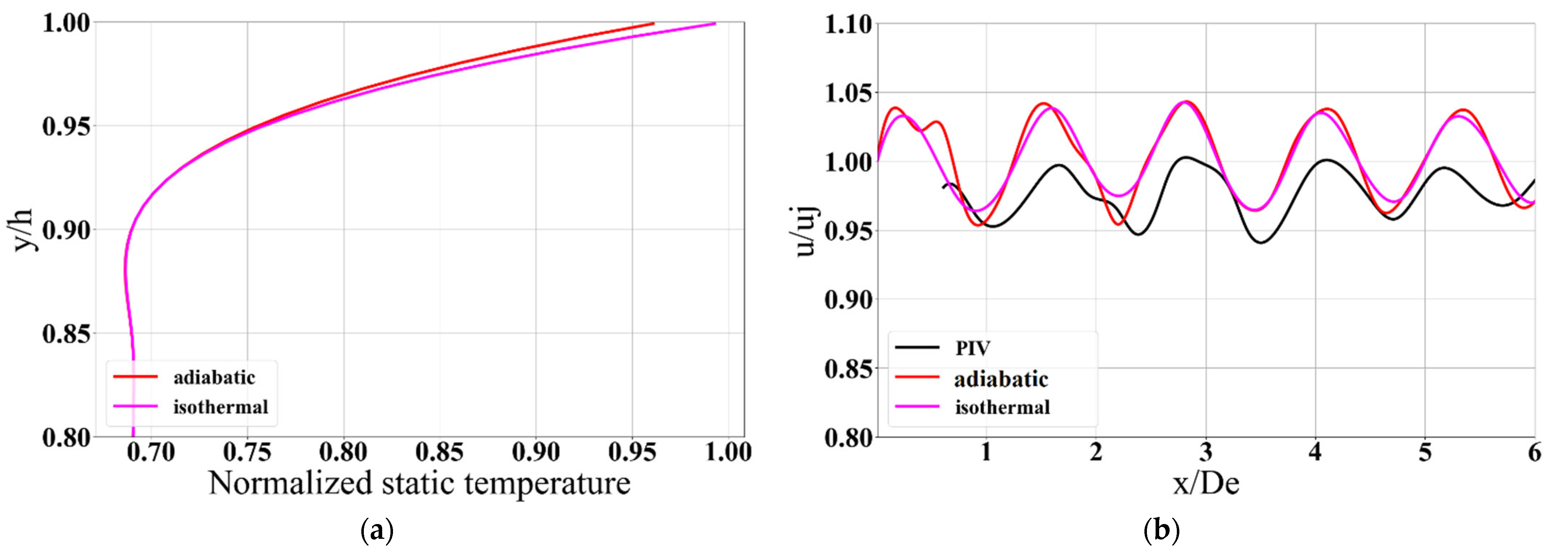
3.2.2. Adiabatic vs. Isothermal Walls

This section evaluates the effect of adiabatic and isothermal nozzle walls. For the isothermal wall case, the wall temperature is maintained at the ambient value. Figure 10a,b show the nozzle exit temperature profiles and jet centerline velocities for both cases. In Figure 10a, the temperature is normalized by ambient temperature and plotted radially at nozzle exit. The y co-ordinate is normalized by nozzle-height (h) at nozzle exit. As seen, the adiabatic case does not reach a value of 1. However, this does not significantly impact the centerline velocity predictions.

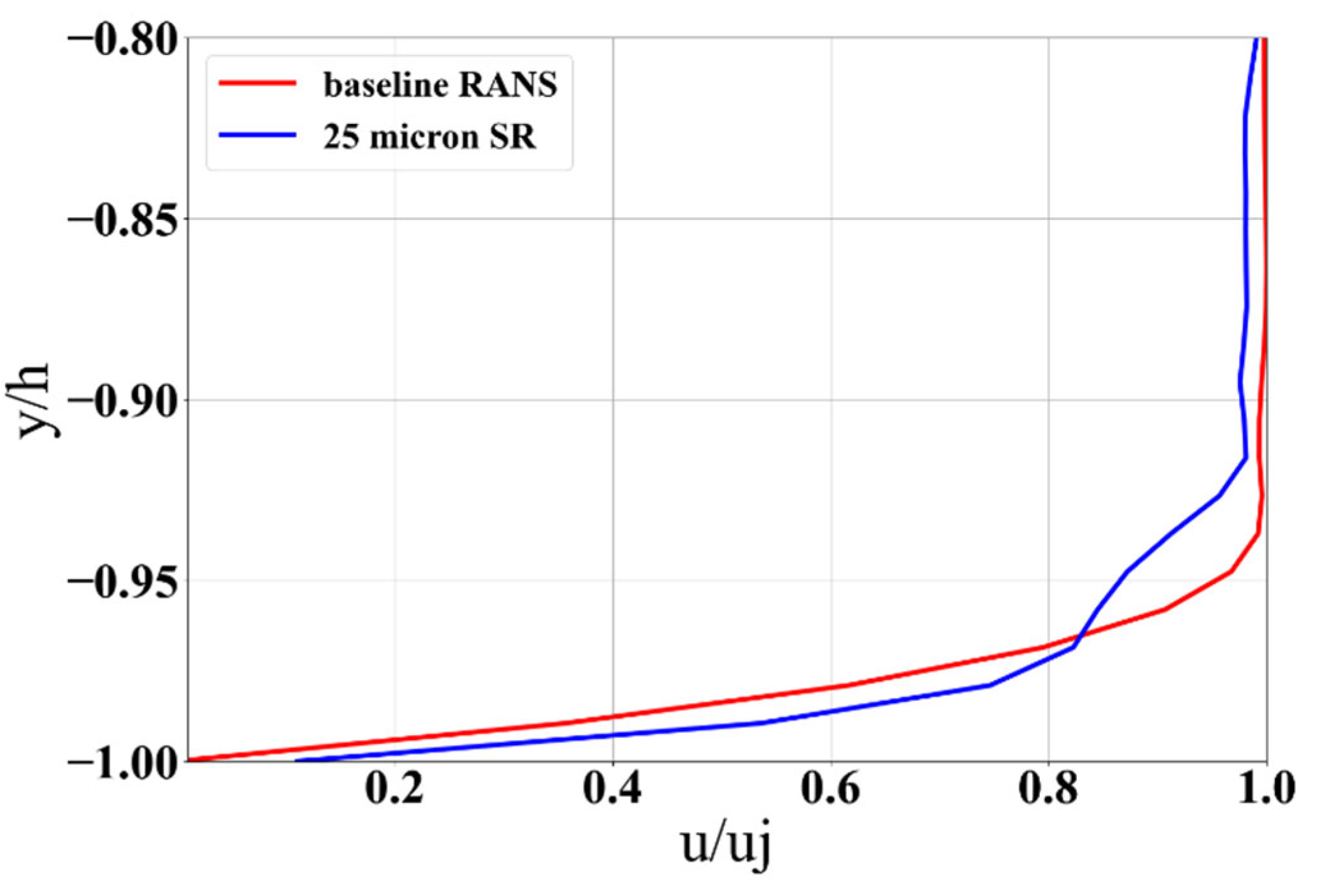
3.3. Wall Surface Roughness

The role of surface roughness is to promote turbulence in boundary layer. This effect becomes crucial in shock boundary layer interactions where stronger shocks can cause boundary layer separation. Numerical simulations can capture these effects if the surface roughness is known. Therefore, this subsection addresses the effect of surface roughness on boundary layer flow and jet by comparing smooth vs. rough walls with 25-micron surface roughness (SR). Understanding the effect of surface roughness on flow physics defines the relationship between turbulence modeling and the geometry. SR causes initial flow disturbance by enhancing the turbulence and affects jet mixing downstream. In some experimental or simulation setups, the boundary layer is tripped to create initial disturbance, for example, by creating protrusion on the modeled geometry or by directly accounting for the value of SR. An investigation of surface roughness with a value of 25 microns based on previous literature [19] in RANS is shown to affect the jet centerline velocity prediction by up to 7% compared to the baseline case with smooth walls. Figure 11 shows the nozzle exit boundary layer profiles for smooth and rough walls. The case with roughness value has a thicker boundary layer, while the case with smooth wall has a thinner boundary layer resulting in lower loss of momentum in the boundary layer. This leads to mixing at a later stage in the baseline case as in Figure 12. Figure 12a shows its effect primarily in the mixing region rather than the region of initial shock cells. Figure 12b takes a closer look at the initial shock cell region, where the velocity oscillation amplitude reduces for the case with upstream duct and surface roughness value. Clearly, surface roughness plays a key role in capturing the velocity oscillation amplitude.

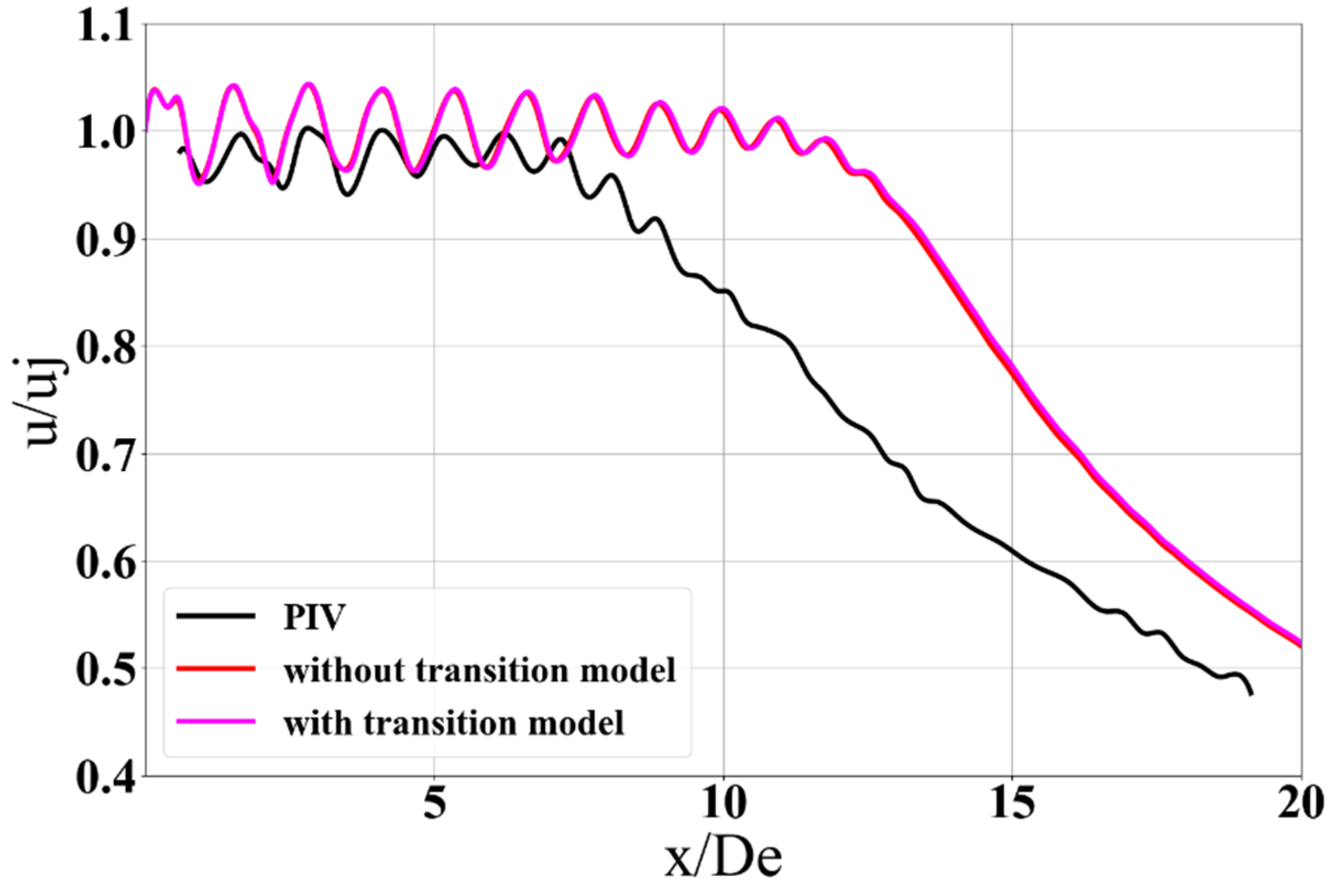
3.4. Laminar to Turbulent Transition

A transition model in combination with a turbulence model predicts the onset of transition in a turbulent boundary layer. Based on the previous literature by Hu et al. [23], small change in transition location near throat region had substantial global effects on the computed results downstream. Considering this, transition model is assessed in the current simulation. It is challenging to determine the location of the transition in an experimental setup. Therefore, a truly predictive capability is required to predict the transition location. In Star-CCM+, Gamma-ReTheta model has the capability of predicting the location of laminar-to-turbulent transition [61]. Gamma-ReTheta Transition model and Gamma Transition models are based on correlations and solve additional transport equations that are coupled with the k-omega SST turbulence model. Most transition models are based on the concept of intermittency—a measure of the amount of time during which the flow is turbulent. An intermittency value of 1 corresponds to a fully turbulent flow (100% percent of the time) and an intermittency value of 0 corresponds to a fully laminar flow. Figure 13 compares the jet centerline velocity obtained with and without transition model. It appears that in current simulations, it does not have significant impact on the jet centerline velocity since the nozzle exit boundary layers are already turbulent.

4. Results—LEVM, NLEVM, RSM and LES

4.1. Turbulence Capture in RANS

Turbulence capture using linear and non-linear eddy viscosity model and Reynolds stress model in RANS is presented. The non-linear eddy viscosity model is based on quadratic constitutive relation suggested by Spalart [35] and is used in combination with Menter’s k-omega SST turbulence model. The Reynolds stress model is based on linear pressure–strain relation suggested by Gibson and Launder [36]. Additionally, comparison with LES is presented in a later section. LES is based on WALE subgrid-scale model suggested in [65].

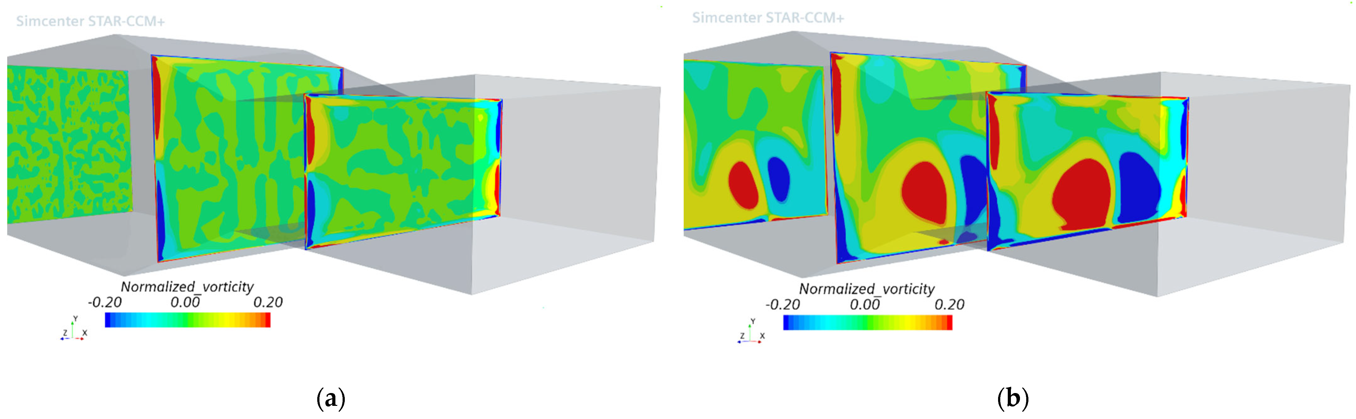
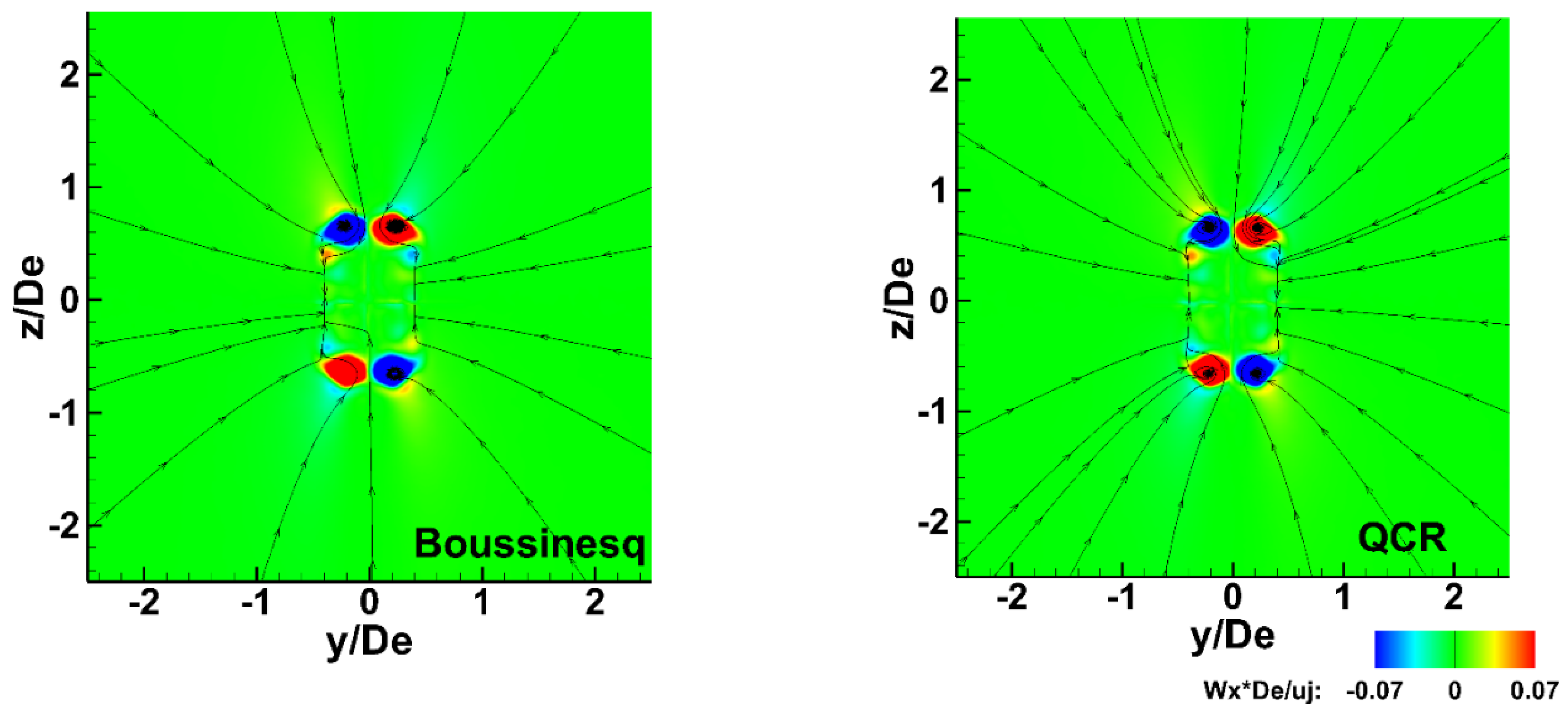
4.1.1. Streamwise Vorticity in Linear vs. Non-Linear Eddy Viscosity RANS

This section briefly describes the results of Boussinesq vs. non-linear eddy viscosity (QCR) approach in RANS. The results are presented using Menter’s k-omega SST turbulence model. From Figure 14, enhanced regions of streamwise vorticity can be seen. Figure 14 shows the comparison of normalized magnitudes of streamwise vorticity at x/De = 1, 8.9 for Boussinesq RANS (left) and QCR RANS (right). These locations are chosen such that one of them is immediately downstream of the nozzle exit and the other is just after the end of potential core. The role of QCR is to promote the vorticity in the jet a few diameters downstream of the nozzle exit which helps jet mixing.

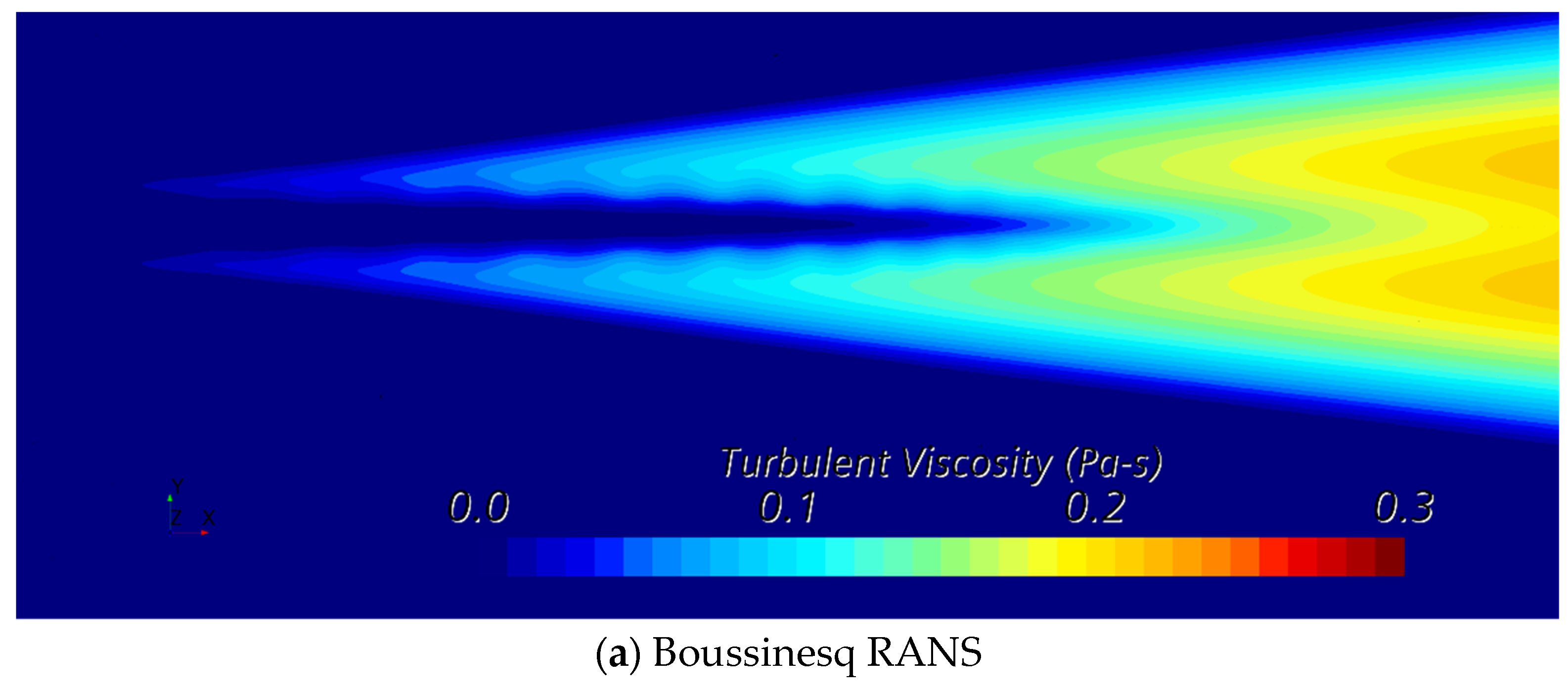
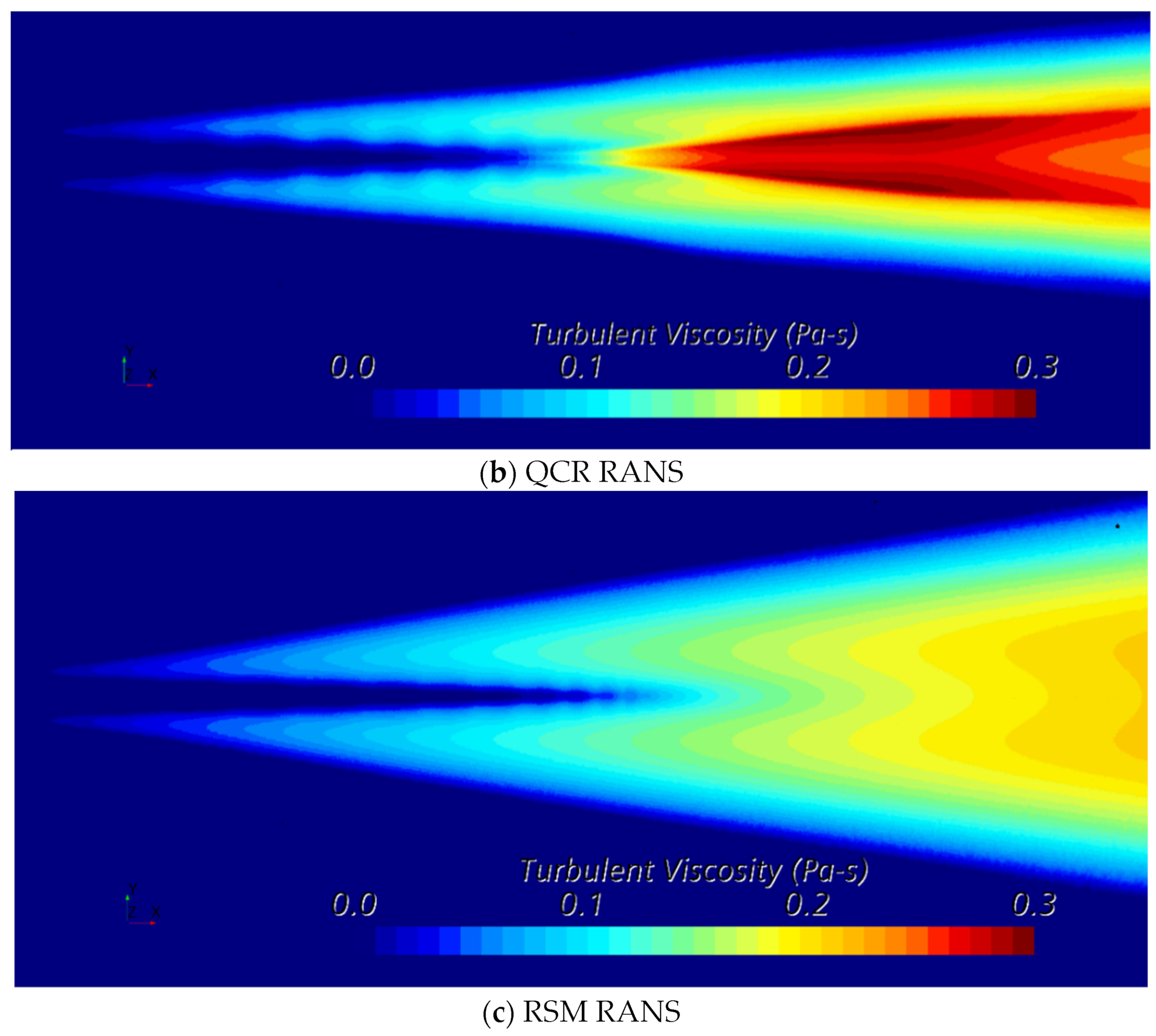
4.1.2. Turbulent Viscosity in RANS

Figure 15 shows the turbulent viscosity contours downstream of the nozzle for Boussinesq RANS, QCR RANS and RSM RANS. As seen, the magnitudes of turbulent viscosity increase in the mixing region, after the potential core damp out. In Boussinesq RANS (Figure 15a), the contours show a longer potential core, while Figure 15b for QCR RANS shows a shorter potential core which is the result of enhanced streamwise vorticity magnitudes in QCR RANS as discussed in previous subsection. Therefore, the turbulent viscosity has significantly higher magnitudes in the mixing region. Figure 15c shows the same for RSM. The lower magnitudes of turbulent viscosity are due to the fact that RSM simulation shows higher number of oscillations in the jet centerline velocity which cause the mixing at a later stage as explained in the next subsection. Since turbulent (eddy) viscosity is used to correlate the Reynolds stresses to mean strain rate, it is present in the regions of shear layers and mixing region, i.e. in the region of turbulence and has near zero magnitudes in the region of jet potential core.

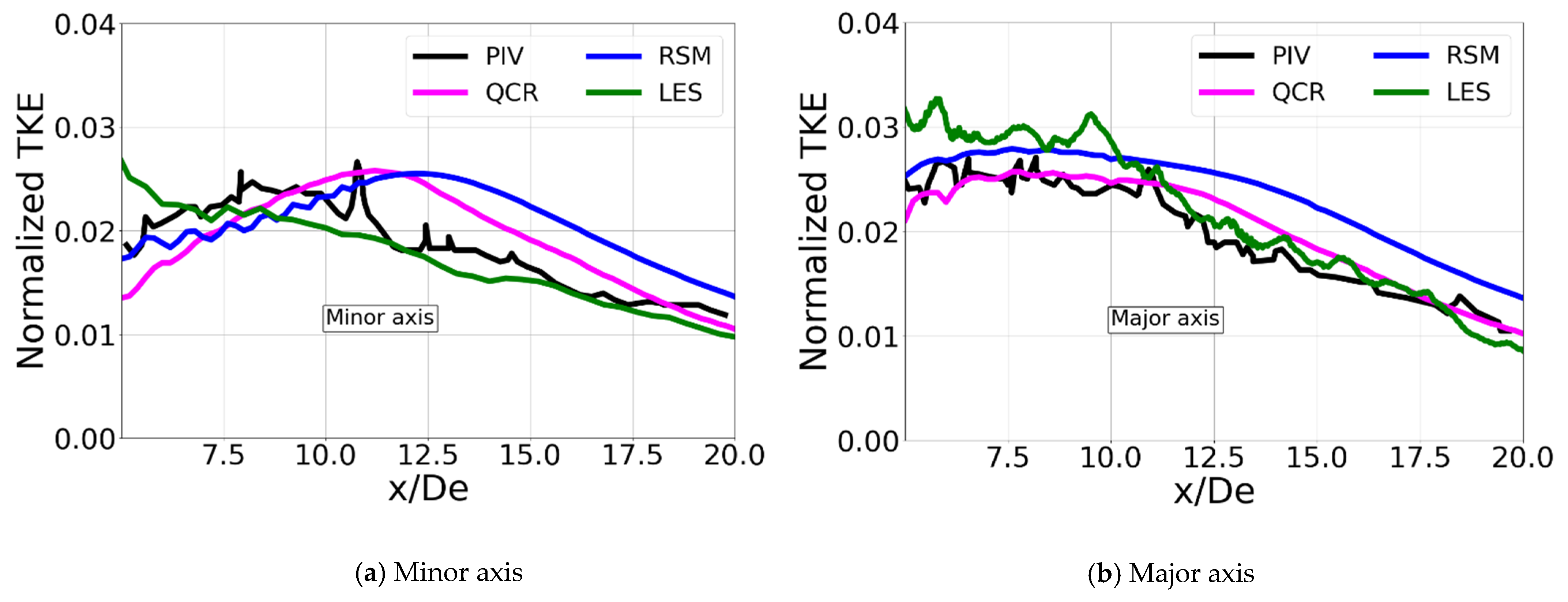
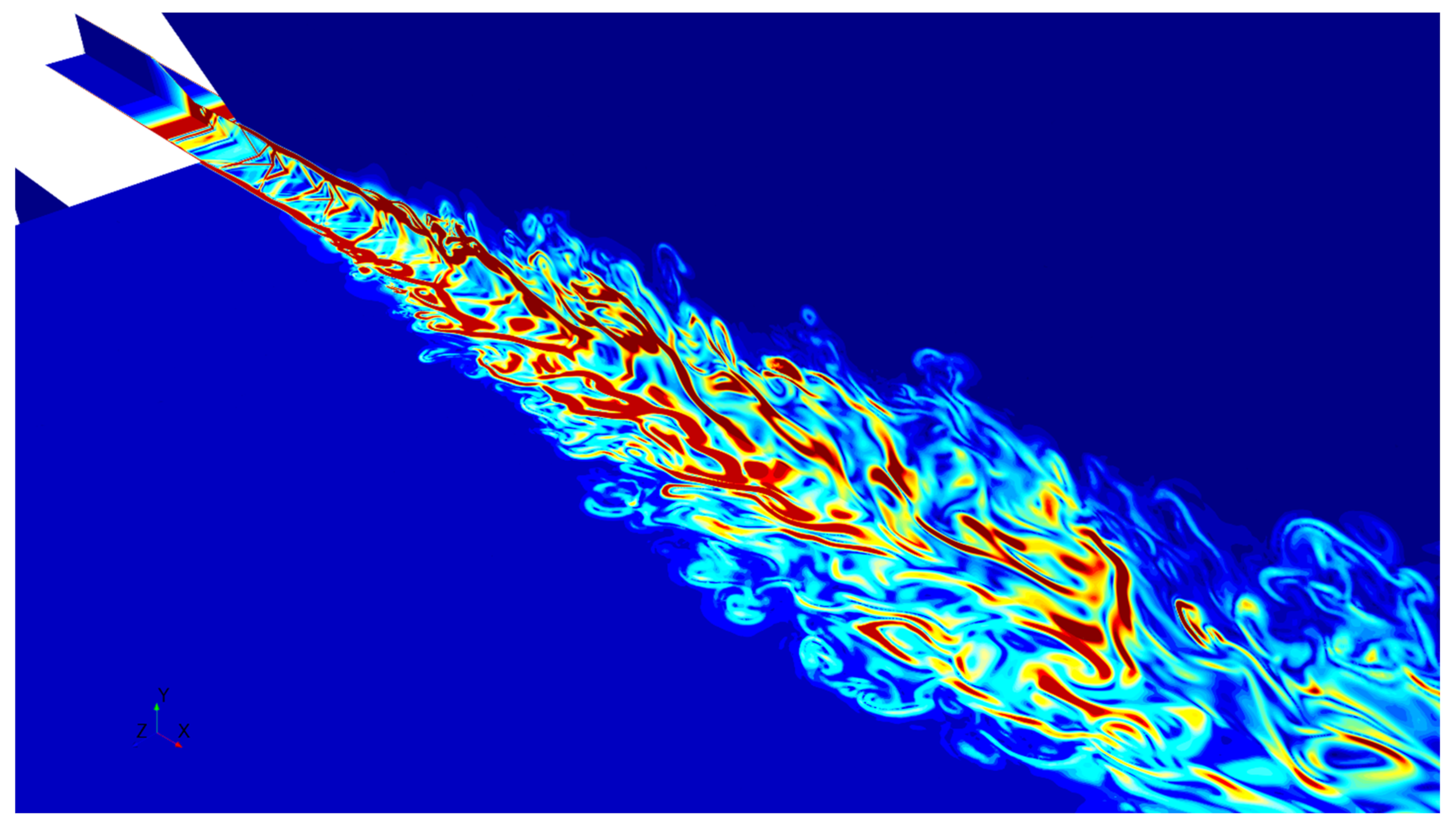
4.2. Comparisons with LES

This section discusses the comparisons of RANS simulations with LES. Additionally, effect of upstream supply duct is also considered in LES. Therefore, two LES simulations are presented, LES without the upstream supply duct (73 million mesh count) and another LES with upstream supply duct (98 million mesh count). Figure 16 indicates the LES grid near nozzle exit and downstream from minor axis plane of view.

Figure 17 compares the jet centerline velocities obtained from Boussinesq (BSQ) RANS, QCR RANS, RSM RANS and LES without upstream supply duct. As seen, QCR RANS and RSM RANS align closely with each other, except that RSM shows greater oscillation of centerline velocity, whereas Boussinesq (baseline) RANS show a larger potential core which clearly underpredicts the mixing. LES agrees closely with experimental data. A closer look at LES with experimental data is provided in Figure 18. The mean absolute percentage error between LES and experimental centerline velocity is 3%.

Figure 18 shows the centerline velocity comparisons for LES cases with and without the upstream supply duct. As seen, they do not show significant differences in velocity oscillations amplitude or in the length of potential core. Apart from considerations in LES, uncertainty coming from PIV experimental data is one of the important topics as discussed in [63,64,66,67]. PIV-based measurements are prone to uncertainty in the regions with high velocity gradients such as shear layers as discussed in [67]. Considering this, the current LES results agree quite well with the location shock cells; however, the amplitudes are greater than those of experimental data. The current work does not use synthetic turbulence generation at the nozzle inlet and results in lower turbulence immediately after the nozzle exit causing larger amplitudes of velocity oscillations in LES.

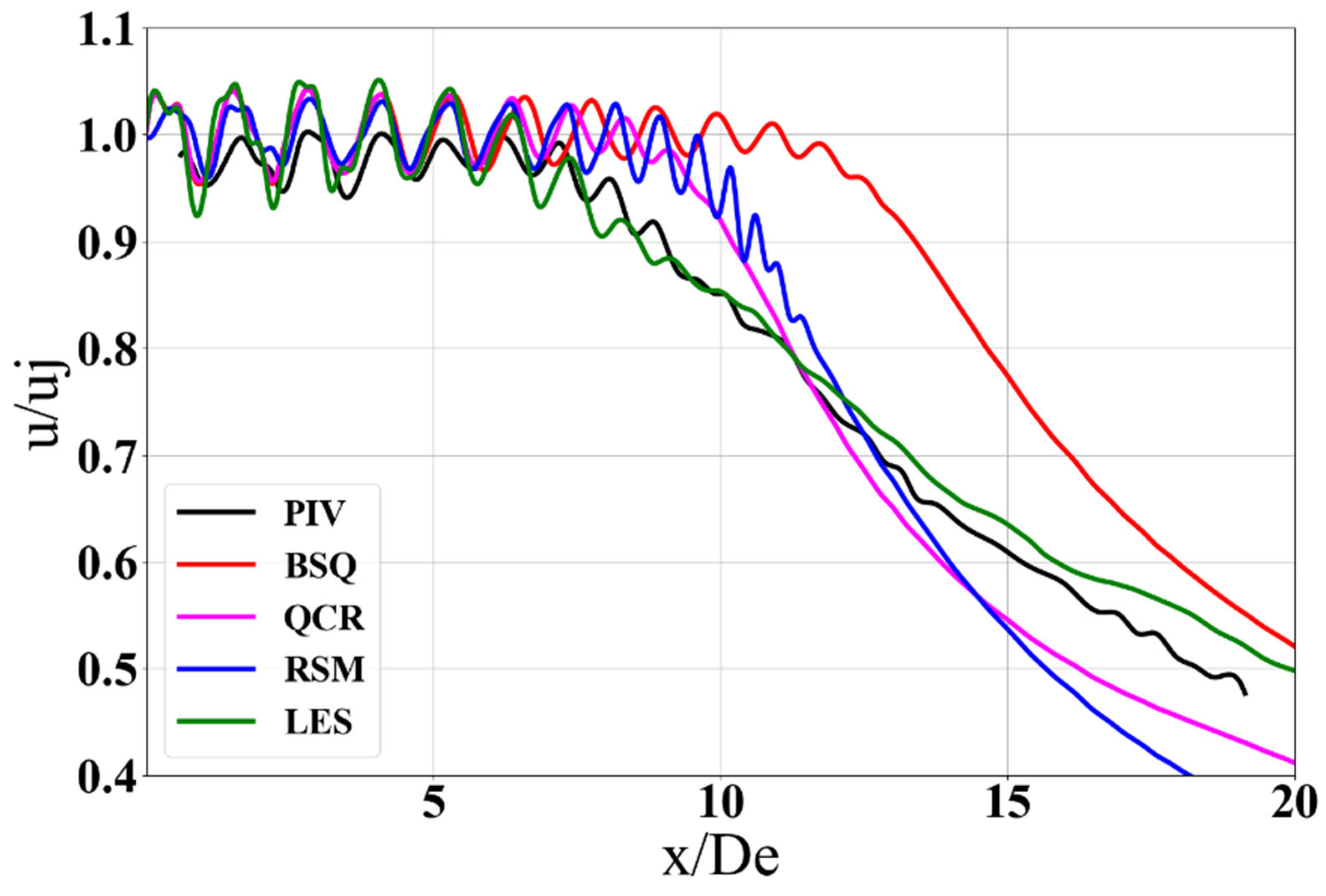
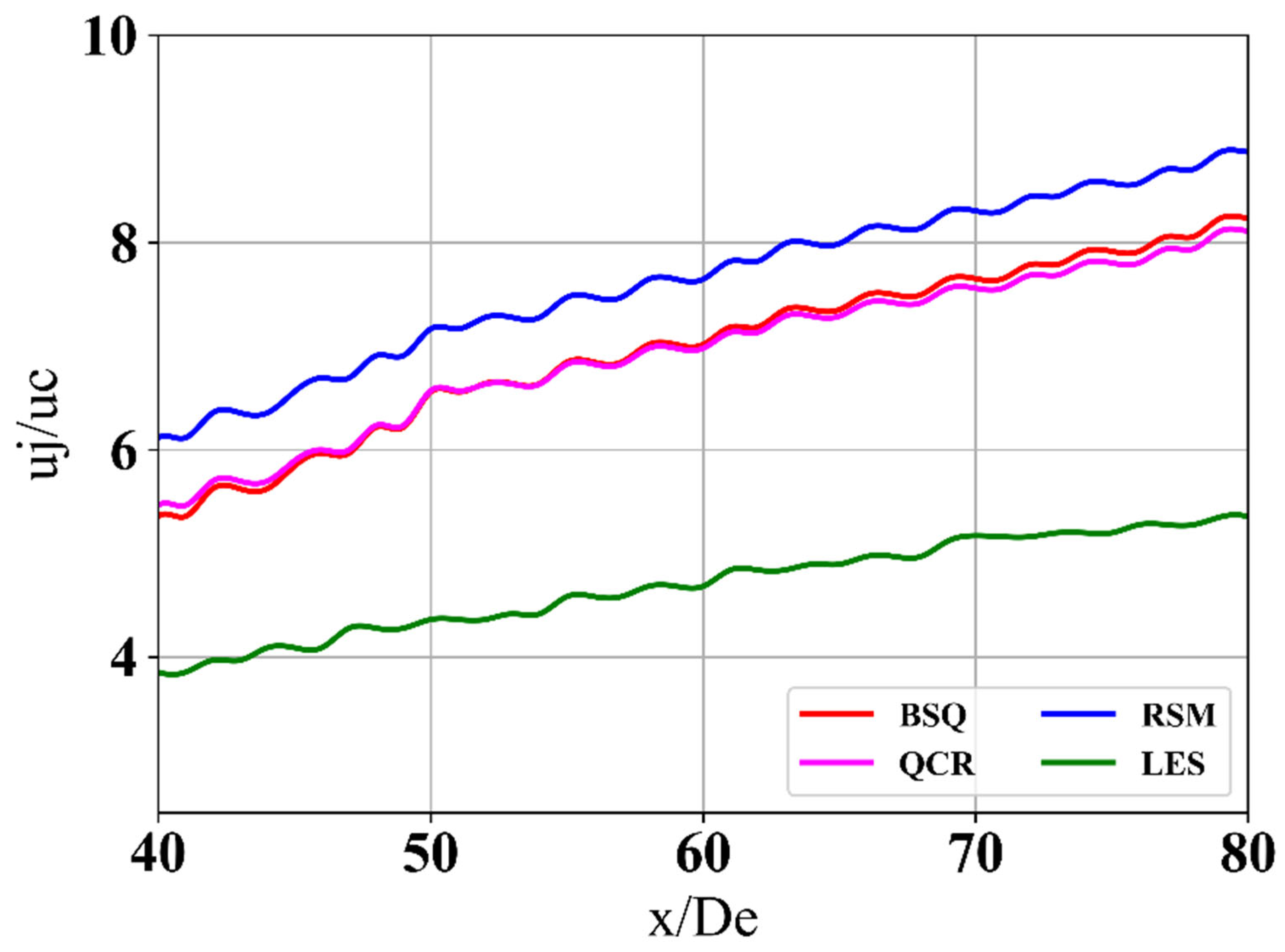
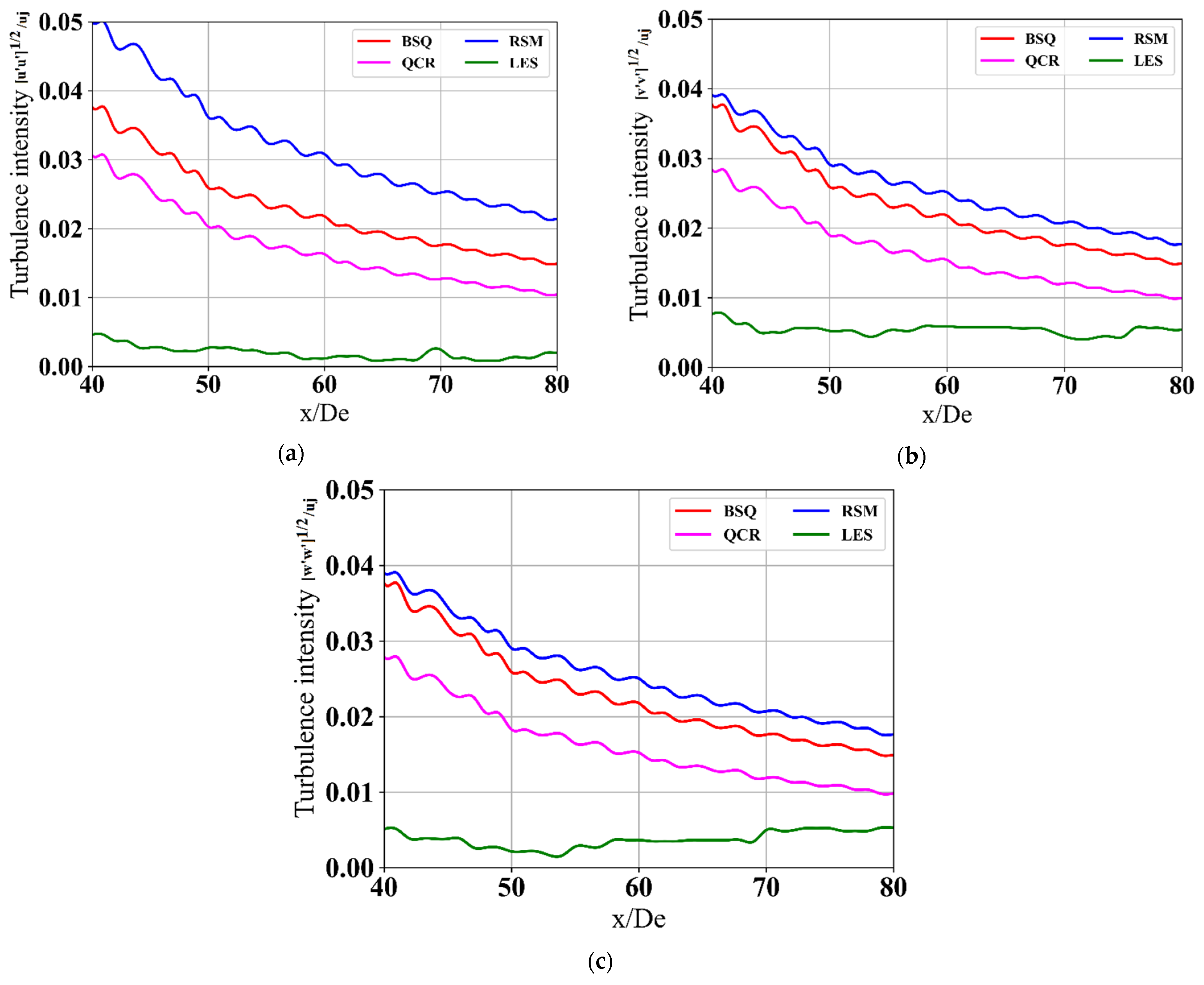
4.2.1. Jet Self-Similarity Assessment

Self-similar behavior is a peculiar property of jets which can be translated as when the inverse of jet centerline velocities increase linearly independent of streamwise location and when the centerline turbulence intensities remain constant along the jet axis [68,69]. Prior works [70] have reported the existence of self-similarity in rectangular jets. In order to assess the self-similarity, the centerline mean flow and turbulence intensities in both RANS and LES are evaluated. Figure 19 shows the inverse of jet centerline velocity normalized with jet exit velocity at nozzle exit. As seen, it increases linearly with the streamwise location in all simulation fidelities. BSQ, QCR and RSM RANS follow the same slope while LES indicates a relatively moderate slope.

Figure 20 shows the turbulence intensities along jet centerline for all simulation fidelities comparing all three components. The turbulent flow in RANS simulations does not obtain constant values of the three components of turbulence intensities and therefore, it appears that it does not reach self-similarity, whereas LES turbulence intensities become constant 40 diameters downstream of the nozzle exit. Therefore, it appears that LES turbulent flow reaches self-similarity past this location.

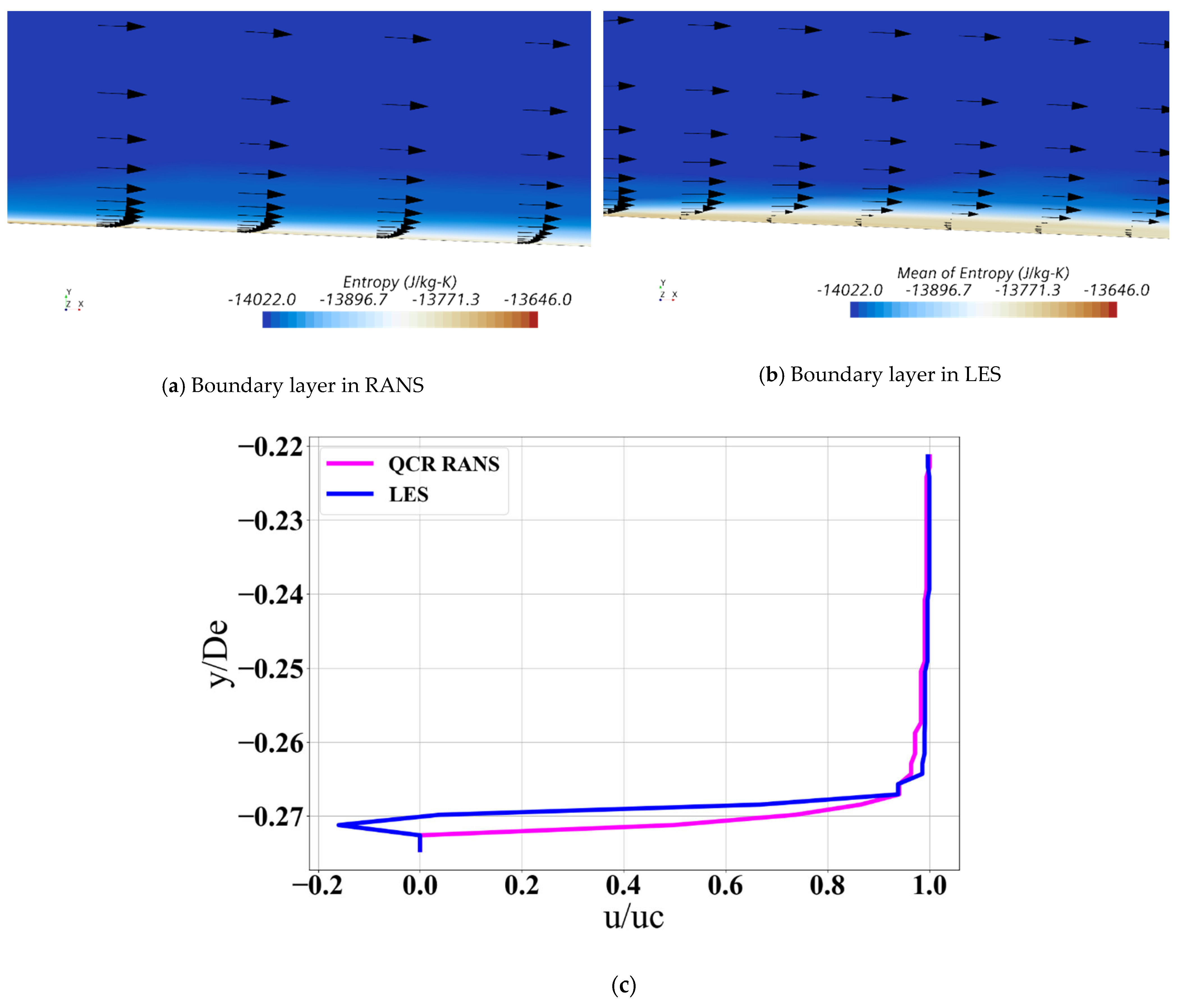
4.2.2. Boundary Layer Growth in RANS and LES

Boundary layer growth is an important factor in the jet development downstream. Many researchers have emphasized that the nozzle exit boundary layer plays a significant role in capturing the physics accurately in numerical simulations. Therefore, differences in RANS vs. LES are shown here to highlight the boundary layer growth. For comparison purposes, QCR RANS is chosen along with LES. The boundary layer in QCR RANS simulation does not separate but undergoes thickening induced by the throat shock wave as seen in Figure 21a. The contours are colored by entropy calculated as $s=C_{p}ln\left(\frac{T}{T_{ref}}\right)-Rln\left(\frac{P}{P_{ref}}\right)$, where $C_p$ is the specific heat in J/(kg-K), R is the specific gas constant in J/(kg-K), T is temperature in K and T_ref is the reference temperature, P is the absolute pressure in Pa and P_ref is the reference pressure. Star-CCM+ assumes the standard state temperature for an ideal gas as 298.15 K and standard state entropy as 0. Therefore, the entropy calculations are relative to the standard conditions and negative values are possible. Entropy production through boundary layer can be clearly seen from Figure 21a,b. In LES (Figure 21b), the boundary separates due to the throat shock wave just downstream of the throat. We anticipate that this is due to the near-wall grid as well as accounting of the turbulence in RANS vs. LES. In this case, LES resolves the boundary layer since the height of first prism layer falls within the viscous sublayer, leading to wall y+ ~1. Figure 21c shows a line plot at x/De = −1 comparing the boundary layer profiles from RANS and LES which clearly indicates separated boundary layer in LES downstream of the throat.

5. Discussion on Anisotropy

This work describes various factors influencing the anisotropy of turbulence in the jet exiting the nozzle. The geometry of the rectangular nozzle is asymmetric which leads to asymmetry of turbulence. The turbulence modeling choices in RANS, ranging from linear eddy viscosity, non-linear eddy viscosity, Reynolds stress model-based RANS influence the turbulence capture. High-fidelity WALE LES also influences the anisotropy due to the resolved part of the flow field. A closer look at the minor- and major-axis TKE statistics obtained from various modeling choices as well as PIV data shows their resultant behavior. Figure 22a,b show the comparisons of TKE along shear layers on minor and major axis planes. The effect of accounting for Reynolds stress anisotropy is shown in the Figure, thus indicating how each numerical fidelity predicts the second-order turbulence statistics. Figure 23 visualizes the jet turbulence on minor and major axis planes.

6. Conclusions and Future Work

This work demonstrates the considerations for capturing the right physics in numerical simulations. Detailed account of various boundary conditions and turbulence modeling approaches in RANS are presented for rectangular supersonic jet. Nozzle internal flow and external flow are both addressed. The results are qualitatively compared against the PIV experimental data from the literature. Effect of inlet modeling including turbulence intensity and upstream supply duct is addressed. Effect of number of prism layers in boundary layer mesh is addressed by closely looking at nozzle exit boundary layer profiles. It is shown that lower number of prism layers results in higher boundary layer thickness, which affects the centerline velocity prediction downstream of the nozzle exit. Specifically, the number of prism layers and wall y+ values impact the wall shear stress prediction and thus the nozzle exit boundary layer profiles. This in turn affects the centerline velocity predictions in the mixing region. However, their effect on the first few shock cells is minimal. Similarly, effect of isothermal vs. adiabatic wall modeling is demonstrated. Effect of surface roughness on nozzle internal flow physics is evaluated. The role of surface roughness is to thicken the boundary layer at nozzle exit causing better mixing of the jet as compared to smooth wall nozzle. It is shown that these factors directly influence the jet centerline velocity prediction. The RANS case with upstream supply duct and with nozzle wall surface roughness directly affects the velocity oscillation amplitude in the vicinity of the nozzle exit and in turn causes an early damp out of potential core. Additionally, laminar to turbulent transition modeling is also addressed; however, since the nozzle internal boundary layer is already turbulent, it does not seem to affect the centerline velocity prediction. To improve the turbulence capture, non-linear eddy viscosity-based SST model and Reynolds stress model are considered. It is shown that NLEVM enhances the streamwise vorticity and thus helps the jet mixing as compared to the linear/Boussinesq RANS. A comparison with Boussinesq RANS shows that NLEVM and RSM significantly improve the predictions. To further assess the wall-bounded flow, boundary layer growth in RANS and LES is presented. It appears that boundary layer in LES undergoes a separation just downstream of the nozzle throat due to the shock wave but re-attaches later. The boundary layer in RANS simulations is attached but undergoes thickening due to the throat shock wave. Jet self-similarity resulting from various numerical simulations is assessed and it is shown that the turbulence becomes self-similar in LES. Finally, a brief discussion on factors influencing the anisotropy in jet turbulence is provided.

In summary, this paper demonstrates various aspects of accuracy improvements in RANS and LES for supersonic flow associated with rectangular jet by closely evaluating their effect on nozzle internal flow as well as external flow downstream of the nozzle exit. Several factors are rigorously assessed and are shown to directly affect the flowfields, which lead to improvements as compared to the baseline case. While the results represent a specific setup of rectangular jet, the factors considered in this research are general enough to be applicable to most CFD studies and the goal here is to highlight their effect by considering a rectangular jet flowfield. A deeper investigation focusing on the boundary conditions, mesh and domain sensitivity, turbulence capture including the effect of linear, non-linear eddy viscosity models and RSM as well as high-fidelity WALE LES is presented.

References

1. Wilcox, D.C. Turbulence Modeling for CFD; DCW Industries: La Canada, CA, USA, 1998; Volume 2. [Google Scholar]
2. Greitzer, E.M.; Tan, C.S.; Graf, M.B. Internal Flow: Concepts and Applications; Cambridge University Press: Cambridge, UK, 2007. [Google Scholar]
3. Schlichting, H.; Kestin, J. Boundary Layer Theory; McGraw-Hill: New York, NY, USA, 1961; Volume 121. [Google Scholar]
4. Shapiro, A.H. The Dynamics and Thermodynamics of Compressible Fluid Flow; Ronald Press: New York, NY, USA, 1953. [Google Scholar]
5. Bobba, C.R.; Ghia, K.N. A study of three-dimensional compressible turbulent jets. In 2nd Symposium on Turbulent Shear Flows; Imperial College of Science and Technology: London, UK, 1979; pp. 1–26. [Google Scholar]
6. Georgiadis, N.J.; DeBonis, J.R. Navier–stokes analysis methods for turbulent jet flows with application to aircraft exhaust nozzles. Prog. Aerosp. Sci. 2006, 42, 377–418. [Google Scholar] [CrossRef]
7. Mihaescu, M.; Semlitsch, B.; Fuchs, L.; Gutmark, E. Assessment of turbulence models for predicting coaxial jets relevant to turbofan engines. In Proceedings of the Conference on Modelling Fluid Flow (CMFF 12), the 15th International Conference on Fluid Flow Technologies, Budapest, Hungary, 4–7 September 2012; pp. 4–7. [Google Scholar]
8. Araya, G. Turbulence model assessment in compressible flows around complex geometries with unstructured grids. Fluids 2019, 4, 81. [Google Scholar] [CrossRef] [Green Version]
9. Rumsey, C.L.; Nishino, T. Numerical study comparing RANS and LES approaches on a circulation control airfoil. Int. J. Heat Fluid Flow 2011, 32, 847–864. [Google Scholar] [CrossRef] [Green Version]
10. Mirjalily, S.A.A. Lambda shock behaviors of elliptic supersonic jets; a numerical analysis with modification of RANS turbulence model. Aerosp. Sci. Technol. 2021, 112, 106613. [Google Scholar] [CrossRef]
11. DeBonis, J.R. Prediction of turbulent temperature fluctuations in hot jets. AIAA J. 2018, 56, 3097–3111. [Google Scholar] [CrossRef]
12. DeBonis, J.R.; Oberkampf, W.L.; Wolf, R.T.; Orkwis, P.D.; Turner, M.G.; Babinsky, H.; Benek, J.A. Assessment of computational fluid dynamics and experimental data for shock boundary-layer interactions. AIAA J. 2012, 50, 891–903. [Google Scholar] [CrossRef]
13. DeBonis, J.R. Evaluation of industry standard turbulence models on an axisymmetric supersonic compression corner. In Proceedings of the 53rd AIAA Aerospace Sciences Meeting, Kissimmee, Florida, 5–9 January 2015; p. 0314. [Google Scholar]
14. Wernet, M.P.; Georgiadis, N.J.; Locke, R.J. Raman temperature and density measurements in supersonic jets. Exp. Fluids 2021, 62, 61. [Google Scholar] [CrossRef]
15. Menter, F.R. Review of the shear-stress transport turbulence model experience from an industrial perspective. Int. J. Comput. Fluid Dyn. 2009, 23, 305–316. [Google Scholar] [CrossRef]
16. Latin, R.M. The Influence of Surface Roughness on Supersonic High Reynolds Number Turbulent Boundary Layer Flow. Ph.D. Thesis, Air Force Institute of Technology, Dayton, OH, USA, 1998. [Google Scholar]
17. Aronson, K.E.; Brezgin, D.V. Wall roughness effect on gas dynamics in supersonic ejector. In AIP Conference Proceedings; AIP Publishing LLC: Melville, NY, USA, 2016; Volume 1770, No. 1; p. 030087. [Google Scholar]
18. Liu, J.; Ramamurti, R. Numerical study of supersonic jet noise emanating from an F404 nozzle at model scale. In Proceedings of the AIAA Scitech 2019 Forum, San Diego, CA, USA, 7–11 January 2019; p. 0807. [Google Scholar]
19. Liu, J.; Khine, Y. Simulations of Nozzle Boundary-Layer Separation in Highly Overexpanded Jets. In Proceedings of the AIAA Aviation Forum, Virtual, 15–19 June 2020. [Google Scholar]
20. Gubanov, D.A.; Dyadâkin, A.A.; Zapryagaev, V.I.; Kavun, I.N.; Rybak, S.P. Experimental investigation of the nozzle roughness effect on the flow parameters in the mixing layer of an axisymmetric subsonic high-velocity jet. Fluid Dyn. 2020, 55, 185–193. [Google Scholar] [CrossRef]
21. Cresci, I.; Ireland, P.T.; Bacic, M.; Tibbott, I.; Rawlinson, A. Realistic velocity and turbulence intensity profiles at the combustor-turbine interaction (CTI) plane in a nozzle guide vane test facility. In Proceedings of the 11th European Conference on Turbomachinery Fluid Dynamics & Thermodynamics, Madrid, Spain, 23–27 March 2015; European Turbomachinery Society: Florence, Italy, 2015. [Google Scholar]
22. Brès, G.A.; Ham, F.; Nichols, J.W.; Lele, S.K. Nozzle wall modeling in unstructured large eddy simulations for hot supersonic jet predictions. In Proceedings of the 19th AIAA/CEAS Aeroacoustics Conference, Berlin, Germany, 27–29 May 2013; p. 2142. [Google Scholar]
23. Bres, G.A.; Towne, A.; Lele, S.K. Investigating the effects of temperature non-uniformity on supersonic jet noise with large-eddy simulation. In Proceedings of the 25th AIAA/CEAS Aeroacoustics Conference, Delft, The Netherlands, 20–23 May 2019; p. 2730. [Google Scholar]
24. Bogey, C.; Marsden, O.; Bailly, C. Influence of initial turbulence level on the flow and sound fields of a subsonic jet at a diameter-based Reynolds number of 105. J. Fluid Mech. 2012, 701, 352–385. [Google Scholar] [CrossRef]
25. Upadhyay, P.; Zaman, K.Q. The effect of incoming boundary layer characteristics on the performance of a distributed propulsion system. In Proceedings of the AIAA SciTech 2019 Forum, San Diego, CA, USA, 7–11 January 2019; p. 1092. [Google Scholar]
26. Hu, J.; Rizzi, A. Turbulent flow in supersonic and hypersonic nozzles. AIAA J. 1995, 33, 1634–1640. [Google Scholar] [CrossRef]
27. Siddappaji, K.; Turner, M.G.; Dey, S.; Park, K.; Merchant, A. Optimization of a 3-Stage Booster: Part 2—The Parametric 3D Blade Geometry Modeling Tool. In Turbo Expo: Power for Land, Sea, and Air; American Society of Mechanical Engineers: San Antonio, TX, USA, 2011; Volume 54679, pp. 1431–1443. [Google Scholar]
28. Siddappaji, K. Parametric 3D Blade Geometry Modeling Tool for Turbomachinery Systems. Master’s Thesis, University of Cincinnati, Cincinnati, OH, USA, 2012. [Google Scholar]
29. Siddappaji, K.; Turner, M.G. Versatile Tool for Parametric Smooth Turbomachinery Blades. Aerospace 2022, 9, 489. [Google Scholar] [CrossRef]
30. Siddappaji, K.; Turner, M.G. An Advanced Multifidelity Multidisciplinary Design Analysis Optimization Toolkit for General Turbomachinery. Processes 2022, 10, 1845. [Google Scholar] [CrossRef]
31. Semlitsch, B.; Cuppoletti, D.R.; Gutmark, E.J.; Mihăescu, M. Transforming the shock pattern of supersonic jets using fluidic injection. AIAA J. 2019, 57, 1851–1861. [Google Scholar] [CrossRef] [Green Version]
32. Hafsteinsson, H.E.; Eriksson, L.E.; Andersson, N.; Cuppoletti, D.R.; Gutmark, E. Noise control of supersonic jet with steady and flapping fluidic injection. AIAA J. 2015, 53, 3251–3272. [Google Scholar] [CrossRef]
33. Semlitsch, B.; Mihăescu, M. Fluidic injection scenarios for shock pattern manipulation in exhausts. AIAA J. 2018, 56, 4640–4644. [Google Scholar] [CrossRef]
34. Schmitt, F.G. About Boussinesq’s turbulent viscosity hypothesis: Historical remarks and a direct evaluation of its validity. Comptes Rendus Mécanique 2007, 335, 617–627. [Google Scholar] [CrossRef] [Green Version]
35. Spalart, P.R. Strategies for turbulence modelling and simulations. Int. J. Heat Fluid Flow 2000, 21, 252–263. [Google Scholar] [CrossRef]
36. Gibson, M.M.; Launder, B.E. Ground effects on pressure fluctuations in the atmospheric boundary layer. J. Fluid Mech. 1978, 86, 491–511. [Google Scholar] [CrossRef]
37. Speziale, C.G.; Sarkar, S.; Gatski, T.B. Modelling the pressure–strain correlation of turbulence: An invariant dynamical systems approach. J. Fluid Mech. 1991, 227, 245–272. [Google Scholar] [CrossRef]
38. Sarkar, S.; Lakshmanan, B. Application of a Reynolds stress turbulence model to the compressible shear layer. AIAA J. 1991, 29, 743–749. [Google Scholar] [CrossRef] [Green Version]
39. Mehdizadeh, O.Z.; Temmerman, L.; Tartinville, B.; Hirsch, C. Applications of earsm turbulence models to internal flows. In Turbo Expo: Power for Land, Sea, and Air; American Society of Mechanical Engineers: San Antonio, TX, USA, 2012; Volume 44748, pp. 2079–2086. [Google Scholar]
40. Nagapetyan, H.J. Development and Application of Quadratic Constitutive Relation and Transition Crossflow Effects in the Wray-Agarwal Turbulence Model; Washington University: St. Louis, MO, USA, 2018. [Google Scholar]
41. Thomas, B.; Agarwal, R.K. Evaluation of various RANS turbulence models for predicting the drag on an Ahmed body. In Proceedings of the AIAA Aviation 2019 Forum, Dallas, TX, USA, 17–21 June 2019; p. 2919. [Google Scholar]
42. Rumsey, C.L.; Carlson, J.R.; Pulliam, T.H.; Spalart, P.R. Improvements to the quadratic constitutive relation based on NASA juncture flow data. AIAA J. 2020, 58, 4374–4384. [Google Scholar] [CrossRef]
43. Bosco, A.; Reinartz, B.; Brown, L.; Boyce, R. Investigation of a compression corner at hypersonic conditions using a reynolds stress model. In Proceedings of the 17th AIAA International Space Planes and Hypersonic Systems and Technologies Conference, San Francisco, CA, USA, 11–14 April 2011; p. 2217. [Google Scholar]
44. Molchanov, A.M.; Myakochin, A.S. Numerical simulation of high-speed flows using the algebraic Reynolds stress model. Russ. Aeronaut. 2018, 61, 236–243. [Google Scholar] [CrossRef]
45. Gao, F. Advanced Numerical Simulation of Corner Separation in a Linear Compressor Cascade. Ph.D. Thesis, Ecole Centrale de Lyon, Écully, France, 2014. [Google Scholar]
46. Yoder, D.A. Assessment of Turbulence Models for a Single-Injector Cooling Flow. In Proceedings of the AIAA SCITECH 2022 Forum, San Diego, CA, USA, 3–7 January 2022; p. 1812. [Google Scholar]
47. Paysant, R.; Laroche, E.; Troyes, J.; Donjat, D.; Millan, P.; Buet, P. Scale resolving simulations of a high-temperature turbulent jet in a cold crossflow: Comparison of two approaches. Int. J. Heat Fluid Flow 2021, 92, 108862. [Google Scholar] [CrossRef]
48. Paysant, R.; Laroche, E.; Millan, P.; Buet, P. RANS modelling of a high-temperature jet in a cold crossflow: From eddy viscosity models to advanced anisotropic approaches. In Proceedings of the AIAA Scitech 2021 Forum, Virtual, 11–15 & 19–21 January 2021; p. 1542. [Google Scholar]
49. Boychev, K.; Barakos, G.N.; Steijl, R. Numerical simulations of multiple shock wave boundary layer interactions. In Proceedings of the AIAA Scitech 2021 Forum, Virtual, 11–15 & 19–21 January 2021; p. 1762. [Google Scholar]
50. Bhide, K.; Siddappaji, K.; Abdallah, S.; Roberts, K. Improved Supersonic Turbulent Flow Characteristics Using Non-Linear Eddy Viscosity Relation in RANS and HPC-Enabled LES. Aerospace 2021, 8, 352. [Google Scholar] [CrossRef]
51. Bhide, K.R.; Abdallah, S. Turbulence statistics of supersonic rectangular jets using Reynolds Stress Model in RANS and WALE LES. In Proceedings of the AIAA AVIATION 2022 Forum, Chicago, IL, USA, 27 June–1 July 2022; p. 3344. [Google Scholar]
52. Dhamankar, N.S.; Blaisdell, G.A.; Lyrintzis, A.S. Overview of turbulent inflow boundary conditions for large-eddy simulations. AIAA J. 2018, 56, 1317–1334. [Google Scholar] [CrossRef]
53. Liu, J.; Corrigan, A.T.; Kailasanath, K.; Taylor, B.D. Impact of the specific heat ratio on the noise generation in a high-temperature supersonic jet. In Proceedings of the 54th AIAA Aerospace Sciences Meeting, San Diego, CA, USA, 4–8 January 2016; p. 2125. [Google Scholar]
54. El Rafei, M.; Könözsy, L.; Rana, Z. Investigation of numerical dissipation in classical and implicit large eddy simulations. Aerospace 2017, 4, 59. [Google Scholar] [CrossRef] [Green Version]
55. Seifollahi Moghadam, Z.; Guibault, F.; Garon, A. On the evaluation of mesh resolution for large-eddy simulation of internal flows using OpenFOAM. Fluids 2021, 6, 24. [Google Scholar] [CrossRef]
56. Bhide, K.; Abdallah, S. Anisotropic Turbulent Kinetic Energy budgets in compressible rectangular jets. Aerospace 2022, 9, 484. [Google Scholar] [CrossRef]
57. Siddappaji, K. On the Entropy Rise in General Unducted Rotors Using Momentum, Vorticity and Energy Transport. Doctoral Dissertation, University of Cincinnati, Cincinnati, OH, USA, 2018. [Google Scholar]
58. Siddappaji, K.; Turner, M. Multifidelity Analysis of a Solo Propeller: Entropy Rise Using Vorticity Dynamics and Kinetic Energy Dissipation. Fluids 2022, 7, 177. [Google Scholar] [CrossRef]
59. Siddappaji, K.; Turner, M. Improved Prediction of Aerodynamic Loss Propagation as Entropy Rise in Wind Turbines Using Multifidelity Analysis. Energies 2022, 15, 3935. [Google Scholar] [CrossRef]
60. Baier, F.; Mora, P.; Gutmark, E.; Kailasanath, K. Flow measurements from a supersonic rectangular nozzle exhausting over a flat surface. In Proceedings of the 55th AIAA Aerospace Sciences Meeting, Grapevine, TX, USA, 9–13 January 2017; p. 0932. [Google Scholar]
61. Simcenter Star-CCM+. Siemens PLM Software, Star-CCM+; Version 15 04.008-R8; Siemens Digital Industries Software: Plano, TX, USA, 2020. [Google Scholar]
62. Bhide, K.; Siddappaji, K.; Abdallah, S. Influence of fluid–thermal–structural interaction on boundary layer flow in rectangular supersonic nozzles. Aerospace 2018, 5, 33. [Google Scholar] [CrossRef] [Green Version]
63. Cuppoletti, D.R. Supersonic Jet Noise Reduction with Novel Fluidic Injection Techniques. Doctoral Dissertation, University of Cincinnati, Cincinnati, OH, USA, 2013. [Google Scholar]
64. Heeb, N.S. Azimuthally Varying Noise Reduction Techniques Applied to Supersonic Jets. Ph.D. Thesis, University of Cincinnati, Cincinnati, OH, USA, 2015. [Google Scholar]
65. Nicoud, F.; Ducros, F. Subgrid-scale stress modelling based on the square of the velocity gradient tensor. Flow Turbul. Combust. 1999, 62, 183–200. [Google Scholar] [CrossRef]
66. Wilson, B.M.; Smith, B.L. Uncertainty on PIV mean and fluctuating velocity due to bias and random errors. Meas. Sci. Technol. 2013, 24, 035302. [Google Scholar] [CrossRef]
67. Lazar, E.; De Blauw, B.; Glumac, N.; Dutton, C.; Elliott, G. A practical approach to PIV uncertainty analysis. In Proceedings of the 27th AIAA Aerodynamic Measurement Technology and Ground Testing Conference, Chicago, IL, USA, 28 June–1 July 2010; p. 4355. [Google Scholar]
68. Pope, S.B.; Pope, S.B. Turbulent Flows; Cambridge University Press: Cambridge, UK, 2000. [Google Scholar]
69. Bogey, C.; Bailly, C. Turbulence and energy budget in a self-preserving round jet: Direct evaluation using large eddy simulation. J. Fluid Mech. 2009, 627, 129–160. [Google Scholar] [CrossRef] [Green Version]
70. Krothapalli, A.; Baganoff, D.; Karamcheti, K. On the mixing of a rectangular jet. J. Fluid Mech. 1981, 107, 201–220. [Google Scholar] [CrossRef]
Figure 1. Rectangular nozzle geometry taken from [60], dimensions in inches.
Fluids 07 00385 g001
Figure 2. Centerline velocity comparison for baseline RANS with PIV data [60].
Fluids 07 00385 g002
Figure 3. Fine RANS mesh.
Fluids 07 00385 g003
Figure 4. Mesh sensitivity study for jet centerline velocity compared with PIV data from [60].
Fluids 07 00385 g004
Figure 5. Domain dependency study compared with PIV data from [60].
Fluids 07 00385 g005
Figure 6. Effect of inflow conditions compared with PIV data from [60]. (a) Effect of turbulence intensity (TI). (b) Effect of upstream air supply duct.
Fluids 07 00385 g006
Figure 7. Contours of normalized streamwise vorticity along crossflow planes inside the nozzle. (a) Without the upstream supply duct. (b) With upstream supply duct.
Fluids 07 00385 g007
Figure 8. Prism layer sensitivity.
Fluids 07 00385 g008aFluids 07 00385 g008b
Figure 9. Prism layer sensitivity. (a) Jet centerline velocity compared with PIV data from [60]. (b) Boundary layer profiles at nozzle exit.
Fluids 07 00385 g009
Figure 10. Effect of adiabatic and isothermal wall modeling on exit temperature profile and jet centerline velocity compared with PIV data from [60]. (a) Nozzle exit temperature profile. (b) Jet centerline velocity.
Fluids 07 00385 g010
Figure 11. Boundary layer at nozzle exit with and without surface roughness.
Fluids 07 00385 g011
Figure 12. Effect of nozzle wall surface roughness on jet centerline velocity compared with PIV data from [60].
Fluids 07 00385 g012
Figure 13. Effect of transition model on jet centerline velocity compared with PIV data from [60].
Fluids 07 00385 g013
Figure 14. Streamwise vorticity contours along cross-flow planes at x/De = 1 (top) and x/De = 8.9 (bottom).
Fluids 07 00385 g014aFluids 07 00385 g014b
Figure 15. Contours of eddy viscosity downstream of the nozzle exit.
Fluids 07 00385 g015aFluids 07 00385 g015b
Figure 16. LES grid: Zoomed-in view near nozzle exit.
Fluids 07 00385 g016
Figure 17. Jet centerline velocity comparison with PIV data from [60]—Boussinesq SST RANS, QCR, RSM and LES.
Fluids 07 00385 g017
Figure 18. Jet centerline velocity comparison with PIV data from [60]—LES with and without upstream duct.
Fluids 07 00385 g018
Figure 19. Centerline profiles of inverse of streamwise velocity.
Fluids 07 00385 g019
Figure 20. Centerline profiles of turbulence intensities, (a) streamwise, (b) radial, (c) spanwise.
Fluids 07 00385 g020
Figure 21. Boundary layer growth downstream of the nozzle throat, indicating (a) attached boundary layer in RANS, (b) separated boundary layer in LES, (c) Line plot at x/De = −1, comparing RANS and LES.
Fluids 07 00385 g021
Figure 22. TKE comparisons on minor- and major-axis shear layers with PIV data from [60].
Fluids 07 00385 g022
Figure 23. LES-based illustration of the jet flowfield on minor and major axis planes.
Fluids 07 00385 g023