A Method for Choosing the Spatial and Temporal Approximations for the LES Approach

Abstract

Analysis and optimization of the hybrid upwind-central numerical methods for modern versions of large eddy simulations (LESs) are presented herein. Optimization was performed based on examination of the characteristics of the spatial and temporal finite-volume approximations of the convective terms of filtered Navier–Stokes equations. A method for selecting level of subgrid viscosity that corresponds to the chosen numerical scheme and makes it possible to obtain an extended inertial interval of the energy spectrum is proposed. A series of LESs of homogeneous isotropic turbulence decay were carried out, and the optimal values of the subgrid model constants included in the hybrid shear stress transport delay detached eddy simulation (SST-DDES) method were determined. A procedure for generating a consistent initial field of subgrid parameters for these simulations is described. The three-stage explicit Runge–Kutta method was demonstrated to be sufficient for stable time integration, while the popular explicit midpoint method was not. The slope of the energy spectrum was shown to be almost independent of the central-difference scheme order and of the mesh spacing when the correct numerical method was applied. Numerical viscosity was found to become much greater than subgrid viscosity when the upwind scheme contributed about 10% or more to the convective flux approximation.

1. Introduction

The most appropriate approach to resolve turbulent flows is direct numerical simulation (DNS) of instantaneous Navier–Stokes equations. DNS resolves all scales, down to the Kolmogorov microscale. Unfortunately, DNS is a very expensive method that probably will be available for practical problems at the end of the 21st century [1]. Reynolds-averaged Navier–Stokes (RANS) equations are another approach based on modeling all turbulent length scales [2]. RANS modeling only allows description of mean flow structure and is popular in industrial applications. The intermediate approach is large eddy simulation (LES) [3,4,5], which resolves large, turbulent scales directly and models small scales. The latter can be carried out because of Kolmogorov’s hypothesis [6] that at high Reynolds numbers, the turbulent kinetic energy spectrum contains the universal equilibrium interval, and that all eddies that belong to the inertial interval (part of the universal equilibrium interval) are locally isotropic. In addition, it is important that all statistical parameters of these eddies depend only on turbulent kinetic-energy dissipation rate and kinematic viscosity. Nevertheless, LES requires too many computational resources for simulation of wall-bounded flows. According to [1], LES may become widespread in the second half of the 21st century. Thereby, the currently relevant approach is to hybridize these two methods: to use RANS in the near-wall region and LES in the exterior flow. A recent review of hybrid methods is presented in [7]. We will focus on reviewing only one in this paper: namely, detached eddy simulation (DES) [8], which is the most widely used today.

Proper choice of a numerical scheme is a known issue in hybrid methods such as DES and its modern versions [9]. The turbulent flow field in a hybrid simulation can be roughly divided into three regions: a RANS region, a LES region and a buffer area (transition layer between the RANS and LES regions). Central-difference schemes turn out to be unstable in the RANS region, while upwind schemes have a high level of dissipation, which leads to excessive levels of scheme viscosity in the LES region and destruction of small eddies [10]. As a result, turbulent transport description accuracy may decrease significantly. One way to solve this problem is to use hybrid numerical schemes that become upwind in the RANS region and central-difference in the LES region. For example, in [11], convective fluxes are approximated with the use of the second-order upwind scheme for RANS and with the second-order centered scheme for delayed DES (DDES) and improved DDES (IDDES). In addition, [11] demonstrates that subgrid model constants have to be recalibrated with respect to the numerical method. This calibration plays a key role in the LES region because subgrid-scale-model constants influence the dissipation level of a numerical method. Therefore, values of these constants define resolved turbulence scales.

A standard problem in testing numerical methods and subgrid models of LES is decay of homogeneous isotropic turbulence (DHIT)—see [12,13,14,15,16]—due to the fact that the shape of its energy spectrum may be theoretically estimated. Paper [12] proposes using the lattice Boltzmann equation to improve the accuracy of the numerical simulation. The lattice Boltzmann equation modifies eddy viscosity. Additionally, it is worth noting that the impact of the subgrid-scale model has to be reduced in this method through a decrease in the value of the corresponding constant. In [13], the initial field problem was discussed, and an original-solution method was proposed (this method is described below, in the corresponding section). In addition, [13] demonstrates that for a pure central-difference (CD) scheme, the influence of a subgrid model must be increased to reduce the energy accumulation for the high wavenumbers. Further, [13] shows that upwind schemes are too dissipative and need no subgrid model. Paper [14] focuses on subgrid models and their calibration with the help of DNS data. Another method of subgrid model construction is presented in [15], where an artificial neural network (ANN) was used to determine the subgrid-scale stress tensor from the resolved velocity field. The advantage of this approach is that no additional equations or model constants are needed. However, an ANN needs DNS data for training, which may be difficult to obtain in the case of a complex flow structure of industry problems. Several problems were considered in [16], such as the initial field for subgrid parameters, the model constant values for different numerical schemes, and the influence of the upwind part of the hybrid scheme on the turbulent-energy spectrum.

We will focus on the LES region of the DES approach in this paper. A key issue of our research is the correct form of the turbulent-energy spectrum. This problem may be divided into two parts: an investigation of numerical-method influence and the optimal procedure of obtaining a consistent initial field for subgrid model parameters. The results of [16] were taken into account in this study. As is known, in use of an eddy-resolving approach, the solution depends significantly on the chosen numerical method. Today, there is no generally accepted methodology for choosing temporal or spatial approximations. Several of these approximations were considered in this work, and their influence on the numerical solution is investigated. It is worth noting that an approximation of the convective terms is considered in this work. The approximation of the diffusion terms is investigated in [17]. Another concern of this paper is to analyze how the subgrid-scale model interacts with the numerical scheme. It is demonstrated herein that for different schemes, different values of model constants are needed to obtain the correct solution. The procedure of subgrid model constant calibration is described and was applied to all schemes of interest. An additional problem is the consistent initial field of the subgrid model parameters. To solve this problem, the original algorithm was presented. This work is devoted to construction of a correct numerical method for the DDES/IDDES (improved DDES) [11] approach and the difficulties that arise in this case.

This paper is organized as follows: In Section 2, the numerical setup is described. In Section 3, the initial conditions of the test problem are presented. In Section 4, results are discussed, followed by conclusions.

2. Numerical Method and Model

The DES approach, combining the RANS and LES approaches, was used in this paper.

The Reynolds average of an arbitrary function, $a\left(x_k,t\right)$, is defined as follows:

$$\overline{a}(x_i)=\underset{T_t\to \infty }{\lim }\left[\frac{1}{T_t}\underset{t-T_t/2}{\overset{t+T_t/2}{\int }}a(x_i,\tau )d\tau \right],$$

where $T_t$ is an averaging period and $\overline{a}$ is the averaged value. The instantaneous function $a$ could be expressed as the sum of the mean and fluctuating parts: $a=\overline{a}+a^{\prime }$. The Favre average, or density-weighted average, of $a\left(x_k,t\right)$ is defined as $\tilde{a}=\overline{\rho a}/\overline{\rho }$ (here, $\rho$ is density), and the decomposition of the instantaneous function $a$ reads as $a=\tilde{a}+a^{″}$. After Reynolds and Favre averaging, the system of conservation laws may be written as:

$$\frac{\partial u}{\partial t}+\frac{\partial F_i(u)}{\partial x_i}=0,$$

(1)

where $u=\left(\begin{array}{c}\overline{\rho }\\ \overline{\rho }\cdot {\tilde{u}}_k\\ \overline{\rho }\cdot \tilde{E}\end{array}\right)$ is the vector of the conservative variables: $u_k$ is the k-th component of the velocity vector, $E=u_l{u}_l/2+h-p/\rho$ is the total energy, $h=C_{p}T$ is enthalpy and $T$ is temperature, $F_i$ is the flux vector of $u$ in the i-th direction:

$$F_i=\left(\begin{array}{c}\overline{\rho }{\tilde{u}}_i\\ \overline{\rho }{\tilde{u}}_k{\tilde{u}}_i+\overline{p}{\delta }_{ik}+\overline{\rho }\widetilde{u_i^{″}{u}_k^{″}}+{\tilde{\tau }}_{ik}\\ \overline{\rho }\tilde{E}{\tilde{u}}_i+\overline{p}{\tilde{u}}_i+{\tilde{q}}_i+(\overline{\rho }\widetilde{u_i^{″}{u}_k^{″}}+{\tilde{\tau }}_{ik}){\tilde{u}}_k+\overline{\rho }{C}_p\widetilde{T^{″}{u}_k^{″}}\end{array}\right).$$

Here, $p$ is pressure, $C_p$ is heat capacity (a constant value in the tests below) and ${\delta }_{ik}$ is the Kronecker delta. The terms $\overline{\rho }{\tilde{u}}_i$, $\overline{\rho }{\tilde{u}}_k{\tilde{u}}_i+\overline{p}{\delta }_{ik}$ and $\overline{\rho }\tilde{E}{\tilde{u}}_i+\overline{p}{\tilde{u}}_i$ represent the convective fluxes of mass, momentum and energy, respectively. ${\tau }_{ik}$ is the viscous stress tensor:

$${\tau }_{ik}=-\mu \cdot \left(\frac{\partial u_i}{\partial x_k}+\frac{\partial u_k}{\partial x_i}-\frac{2}{3}\frac{\partial u_l}{\partial x_l}{\delta }_{ik}\right)\mathrm{and}{\delta }_{ik}=\{\begin{array}{c}0,i\ne k,\\ 1,i=k.\end{array},$$

where $\mu$ is dynamic viscosity and can be calculated using Sutherland’s formula:

$$\mu =1.72\cdot {10}^{-5}\cdot {\left(\frac{T}{273}\right)}^{3/2}\frac{273+122}{T+122}.$$

$q_i$ is the heat flux calculated by Fourier’s law:

$$q_i=-\frac{\mu }{\mathrm{Pr}}{c}_p\frac{\partial T}{\partial x_i}.$$

Here, $\mathrm{Pr}=0.72$ is the molecular Prandtl number. The equation of state reads as $p=\rho R_{0}T/m$, where $R_0$ is the universal gas constant and $m$ is the molar mass of the gas or mixture. To close the written system of governing Equation (1), the Reynolds stress tensor ($\overline{\rho }\widetilde{u_i^{″}{u}_k^{″}}$), the turbulent heat flux vector ($\overline{\rho }{C}_p\widetilde{T^{″}{u}_k^{″}}$) and turbulent kinetic energy ($k=\widetilde{u_l^{″}{u}_l^{″}}/2$) ($k$ enters into the expression for total energy after averaging) have to be modeled.

LES equations are gained through application of the spatial filtering operator to NS equations. The filtered NS equations coincide formally with RANS Equation (1). The former are obtained through substitution of the Reynolds averages with filtered quantities in the latter. The subgrid-scale stress tensor, the subgrid-scale heat flux vector and subgrid-scale kinetic energy also have to be modeled.

In this paper, we used the hybrid SST-DDES model developed in [11]. This model includes two additional equations, Equations (2) and (3) (for $k$ and $\omega$; $\omega$ is characteristic turbulence frequency), which are applied to the RANS region and the subgrid part of the LES region in this paper. As a result, the system equations to solve comprise 7 equations.

Hereinafter, the average and filter symbols are omitted. The SST closure includes the Boussinesq hypothesis for the Reynolds and subgrid-scale stress tensors; for the turbulent and subgrid-scale heat flux vectors,

$$\rho u_i^{″}{u}_k^{″}=\frac{2}{3}\rho k{\delta }_{ik}-{\mu }_t\cdot \left(\frac{\partial u_i}{\partial x_k}+\frac{\partial u_k}{\partial x_i}-\frac{2}{3}\frac{\partial u_l}{\partial x_l}{\delta }_{ik}\right)\mathrm{and}\rho C_p{T}^{″}{u}_i^{″}=-\frac{{\mu }_t}{{\mathrm{Pr}}_{turb}}{C}_p\frac{\partial T}{\partial x_i},$$

where ${\mathrm{Pr}}_{turb}=0.9$ is the turbulent Prandtl number and ${\mu }_t$ is eddy viscosity (expression is given below).

The two supplementary equations for the subgrid-scale turbulent quantities ($k$ and $\omega$) read:

$$\frac{\partial \rho k}{\partial t}+\nabla \left(\rho \overrightarrow{U}k\right)=\nabla \left[\left(\mu +{\sigma }_k{\mu }_t\right)\nabla k\right]+P_k-\rho \frac{\sqrt{k^3}}{l_{DDES}},\mathrm{and}$$

(2)

$$\frac{\partial \rho \omega }{\partial t}+\nabla \left(\rho \overrightarrow{U}\omega \right)=\nabla \left[\left(\mu +{\sigma }_{\omega }{\mu }_t\right)\nabla \omega \right]+2\left(1-F_1\right)\rho {\sigma }_{\omega 2}\frac{\nabla k\nabla \omega }{\omega }+\alpha \frac{\rho }{{\mu }_t}{P}_k-\beta \rho {\omega }^2,$$

(3)

where $l_{DDES}=l_{RANS}-f_d\max (0,l_{RANS}-l_{LES})$, $l_{LES}=C_{DES}{h}_{\max }$, $C_{DES}=C_{DES1}\cdot F_1+C_{DES2}\cdot (1-F_1)$, $F_1=\tanh \left({\arg }_1^4\right),$ and ${\arg }_1=\min \left[\max \left(\frac{\sqrt{k}}{C_{\mu }\omega d_w};\frac{500\nu }{d_w^2\omega }\right);\frac{4\rho k{\sigma }_{\omega 2}}{\max \left(2\rho {\sigma }_{\omega 2}\frac{\nabla k\nabla \omega }{\omega };{10}^{-10}\right)\cdot d_w^2}\right]$; $d_w$ is the distance to the nearest wall.

Here, $h_{\max }$ is the maximum edge length of the cell. The variables $\alpha ,\beta ,{\sigma }_k,{\sigma }_{\omega },C_{DES}$ represent the model functions that smoothly change their values between the two constants, with subscripts 1 (near the wall) and 2 (far away from the wall). The transition is also made using the function $F_1$. The functions $\alpha ,\beta ,{\sigma }_k,{\sigma }_{\omega },C_{DES}$ approach the following limit values:

$$\begin{array}{c}{\alpha }_1=5/9,{\beta }_1=0.075,{\sigma }_{k1}=0.85,{\sigma }_{\omega 1}=0.5,C_{DES1}=0.78,\\ {\alpha }_2=0.44,{\beta }_2=0.0828,{\sigma }_{k2}=1.0,{\sigma }_{\omega 2}=0.856,C_{DES2}=0.61.\end{array}$$

The left-hand side of each equation for $k$ (2) and $\omega$ (3) is the convective flux of the corresponding parameter. The first term in the right-hand side (RHS) of (2) and (3) represents the molecular and turbulent diffusion fluxes, respectively. The second term in the RHS of the equation for $\omega$ is the cross-diffusion flux, which is also used in the definition of $F_1$. The last two terms on the RHS of (2) and (3) are the sources of subgrid/modeled turbulence: production and dissipation. The expression for turbulence production is the following: $P_k=\min \left({\mu }_{t}2S_{ij}{S}_{ij},10C_{\mu }\rho k\omega \right)$, where $C_{\mu }=0.09$ and $S_{ij}=\frac{1}{2}\left(\frac{\partial u_i}{\partial x_j}+\frac{\partial u_j}{\partial x_i}\right)$ is the shear stress tensor. Eddy viscosity, ${\mu }_t$, is defined as

$${\mu }_t=\frac{\rho k}{\omega }\cdot {\left[\max \left(1;\frac{\sqrt{2S_{ij}{S}_{ij}}{F}_2}{0.31\omega }\right)\right]}^{-1},$$

where $F_2=\tan \mathrm{h}\left({\arg }_2^2\right)$ is the near-wall function; ${\arg }_2=\max \left(\frac{2\sqrt{k}}{C_{\mu }\omega d_w};\frac{500\nu }{d_w^2\omega }\right)$.

The RANS/LES transition is implemented with the length scale, $l_{DDES}$, in the turbulence-dissipation term. The RANS length scale is defined as $l_{RANS}=\sqrt{k}/C_{\mu }\omega$, which takes on significant values in the near-wall region (where $k$ is high enough) and tends to zero elsewhere. Thus, $l_{DDES}$ changes between $l_{RANS}$ and $l_{LES}$ with the help of the empiric blending function $f_d=1-\tanh \left[{(20r_d)}^3\right]$, where $r_d=\frac{{\mu }_t/\rho +\nu }{{(0.41d_w)}^2\sqrt{S_{ij}{S}_{ij}+{\mathrm{\Omega }}_{ij}{\mathrm{\Omega }}_{ij}}}$; ${\mathrm{\Omega }}_{ij}=\frac{1}{2}\left(\frac{\partial u_i}{\partial x_j}-\frac{\partial u_j}{\partial x_i}\right)$ is the vorticity tensor.

To select a numerical scheme appropriate for this equation system and to calibrate the closure model constants, decay of the homogeneous isotropic turbulence (DHIT) problem was considered. There are no walls in the DHIT problem. This means that $d_w\to \infty$, hence $f_d\approx 1-\tanh \left(\frac{1}{d_w^6}\right)\approx 1$, $\underset{d_w\to \infty }{\lim }{F}_1\left(d_w\right)=0$, $C_{DES}=C_{DES2}\cdot (1-F_1)$ $+C_{DES1}\cdot F_1\approx C_{DES2}$ and $l_{DDES}=l_{RANS}-f_d\max (0,l_{RANS}-l_{LES})=l_{LES}\approx C_{DES2}{h}_{\max }$. Therefore, subgrid model influence is determined by only one constant: $C_{DES2}$. It is worth noting that DHIT flow is intrinsically unsteady, and the numerical method must take this point into account.

All simulations were carried out using the second-order-accuracy finite-volume method implemented on a multiblock structured mesh. The solver zFlare [18] from the EWT-TsAGI package [19] was used. Diffusion fluxes were determined using a second-order central scheme. For the primitive variables’ value reconstruction on the faces involved in the determination of convective fluxes, the central differences of the 2nd, 4th and 6th orders were used (hereinafter referred to as CD-2, CD-4 and CD-6, respectively; the corresponding expressions are given in [16]), as well as a hybrid scheme that worked as a weighted average between the upwind (weighted essentially non-oscillatory scheme constructed on a 5 point stencil (WENO5) [20] with the monotonicity-preserving correction [21] and the exact Riemann solver [22]) and central-difference (CD-2) approximations of the convective terms, with the weight function, $\sigma$, defined thusly: $F_{\mathrm{conv}}=\sigma \cdot F_{\mathrm{upwind}}+(1-\sigma )\cdot F_{\mathrm{CD}}$. The blending function, $\sigma$, is taken from [23]. CD-4 and CD-6 are implemented as half-sums of the WENO3 and WENO5 reconstructions (with optimal weights), respectively, on the left and right sides of the cell’s face. The approximations obtained in this way coincide with the finite-difference interpolation formulas [24].

The temporal schemes are explicit: namely, the midpoint method, the 3-step Heun’s scheme of the 3rd order and the 5-step strong stability-preserving scheme of the 4th order [25] (hereinafter euler2, heun3 and ssp5, respectively).

The aforementioned DDES based on the SST model [11] with the shear-layer-adapted (SLA) subgrid length-scale [26] was used. It should be noted that in [16], instead of the average (over the neighboring cells) value, <VTM> (vortex tilting measure), the instantaneous value was used. Figure 1 shows the distribution of the weight function, $F_{KH}(\mathrm{VTM})$, which is used in the definition of the subgrid length scale, $\Delta$: $\Delta ={\tilde{\Delta }}_{\omega }\cdot F_{KH}(\mathrm{VTM})$ (see [26]), where ${\tilde{\Delta }}_{\omega }$ depends on mesh spacing and local vorticity alignment relative to the strain-tensor eigenvectors.

3. Computational Mesh and Initial Conditions of the DHIT Problem

In this study, the computational domain was a cube with periodic boundary conditions. The size of the cube was $2\pi L$. The dimensional parameter, $L$, was 1 m. All simulations were performed on uniform meshes, with the number of cells at ${32}^3\approx 33,000$, ${64}^3\approx 262,000$ and ${128}^3\approx 2.1\times {10}^6$.

An important turbulence characteristic in this problem is the shape of the energy spectrum, $E\left(k\right)$. It is defined as an integral of half of the spectrum-tensor trace over a sphere with radius $k$ [27]: $E\left(k\right)=\frac{1}{2}{\displaystyle \underset{S(k)}{∯}{\mathsf{\Phi }}_{ii}\left(\mathit{k}\right)dS(k)}$, where $\mathit{k}$ is a wavenumber: $k=\left|\mathit{k}\right|$. The spectrum tensor is a three-dimensional Fourier transformation of the velocity correlation tensor $R_{ij}\left(\mathit{r}\right)$ (obtained by averaging the product $u_i\left(\mathit{x}\right)u_j\left(\mathit{x}+\mathit{r}\right)$ over the computational domain):

$${\mathsf{\Phi }}_{ij}\left(\mathit{k}\right)=\frac{1}{{\left(2\pi \right)}^3}{\displaystyle \iiint R_{ij}\left(\mathit{r}\right)\exp (-i\mathit{k}\cdot \mathit{r}) dr}\mathrm{and}{R}_{ij}\left(\mathit{r}\right)=\frac{1}{\mathsf{\Omega }}{\displaystyle \underset{\mathsf{\Omega }}{\iiint }{u}_i\left(\mathit{x}\right)u_j\left(\mathit{x}+\mathit{r}\right) dx},$$

where $S(k)$ is the sphere in wavenumber space with radius $k$, and $\mathit{r}$ is the separation vector between the points. At high Reynolds numbers, the spectrum included the Kolmogorov inertial interval [6]: $E\left(k\right)=C_K{\epsilon }^{2/3}{k}^{-5/3}$, where $\epsilon =-\frac{d{E}_k}{dt}$ ($E_k$ is turbulence kinetic energy). The Kolmogorov range is followed by the range of dissipation, with a rapid decrease in $E\left(k\right)$. The initial velocity field was created with a synthetic turbulence generator, which is similar to the generator in [28]. The difference is that in [28], perturbations were continuously generated on one surface, whereas in this paper, they are generated throughout the whole computational domain at the initial moment of time. The perturbation field is represented as a sum of transverse harmonic oscillations. To maximize the quality of the initial field, the wavenumber values of the harmonics were distributed as a geometric progression with a common ratio of 1.001 instead of the standard value of 1.01 [28]. The initial turbulence energy spectrum corresponds to the von Karman model [29]:

$$E(k)=\frac{55}{9\pi }{E}_{k0}{L}_0\frac{{\left(\frac{\alpha L_0}{2\pi }k\right)}^4}{{\left(1+{\left(\frac{\alpha L_0}{2\pi }k\right)}^2\right)}^{17/6}}\mathrm{where}\alpha \approx 1.339,$$

with the following parameters:

• Initial turbulence kinetic energy can be estimated as $E_{k0}=1000m^2{s}^2$. Therefore, characteristic fluctuation velocity is $u^{\prime }=\sqrt{\frac{2}{3}{E}_{k0}}\approx 25.8\frac{m}{s}$ and the turbulent Mach number is $M_t\approx 0.08.$ Thus, the flow can be considered incompressible;
• The integral turbulence scale, $L_0=\pi L/2\approx 1.57\mathrm{m}$, is equal to a quarter of the computational domain length. This is the largest resolved scale because bigger scale eddies would be significantly deformed by the periodic conditions of the cube;
• The turbulent Reynolds number, ${\mathrm{Re}}_{t0}=\frac{\sqrt{E_{k0}}{L}_0}{\nu }\approx 3\times {10}^6$, is sufficiently large for turbulence to form the inertial interval. Resolved velocity scales are inviscid. Unresolved velocity scales contain a fraction of the vortices from the inertial interval and the vortices from the dissipation interval. The scales of the latter are smaller than the numerical grid size;
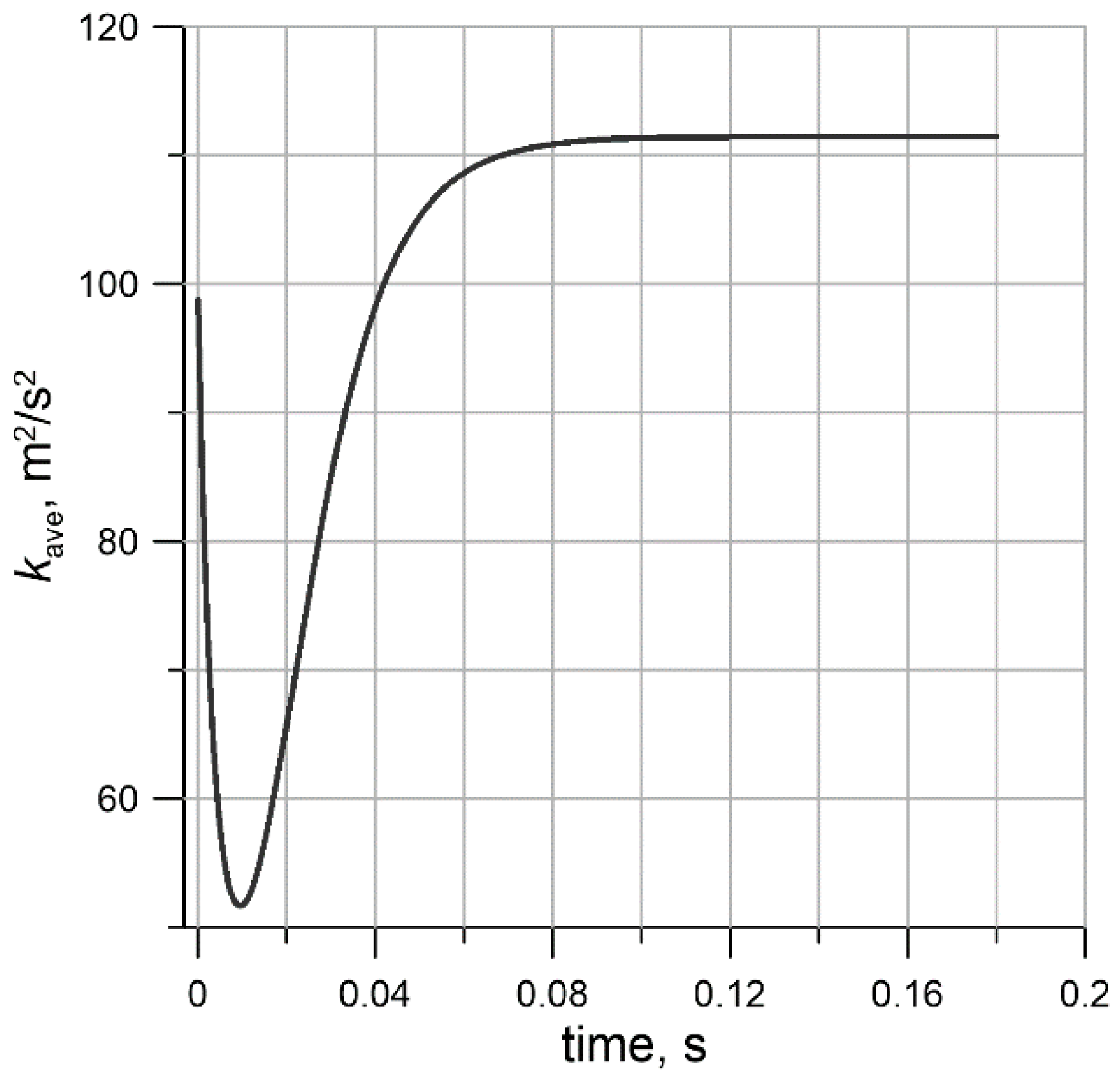
• Initial integral time scale, $T_0$, is estimated as $T_0=L_0/\sqrt{\frac{2}{3}{E}_{k0}}\approx 0.06s$. All simulations are carried out up to physical time $2T_0\approx 0.12s$. The energy spectrum of the turbulence is assumed to reach an equilibrium shape in two large eddy turnover times, and this shape at the final moment of time is determined only by the properties of the subgrid model and the numerical method.

4. Results

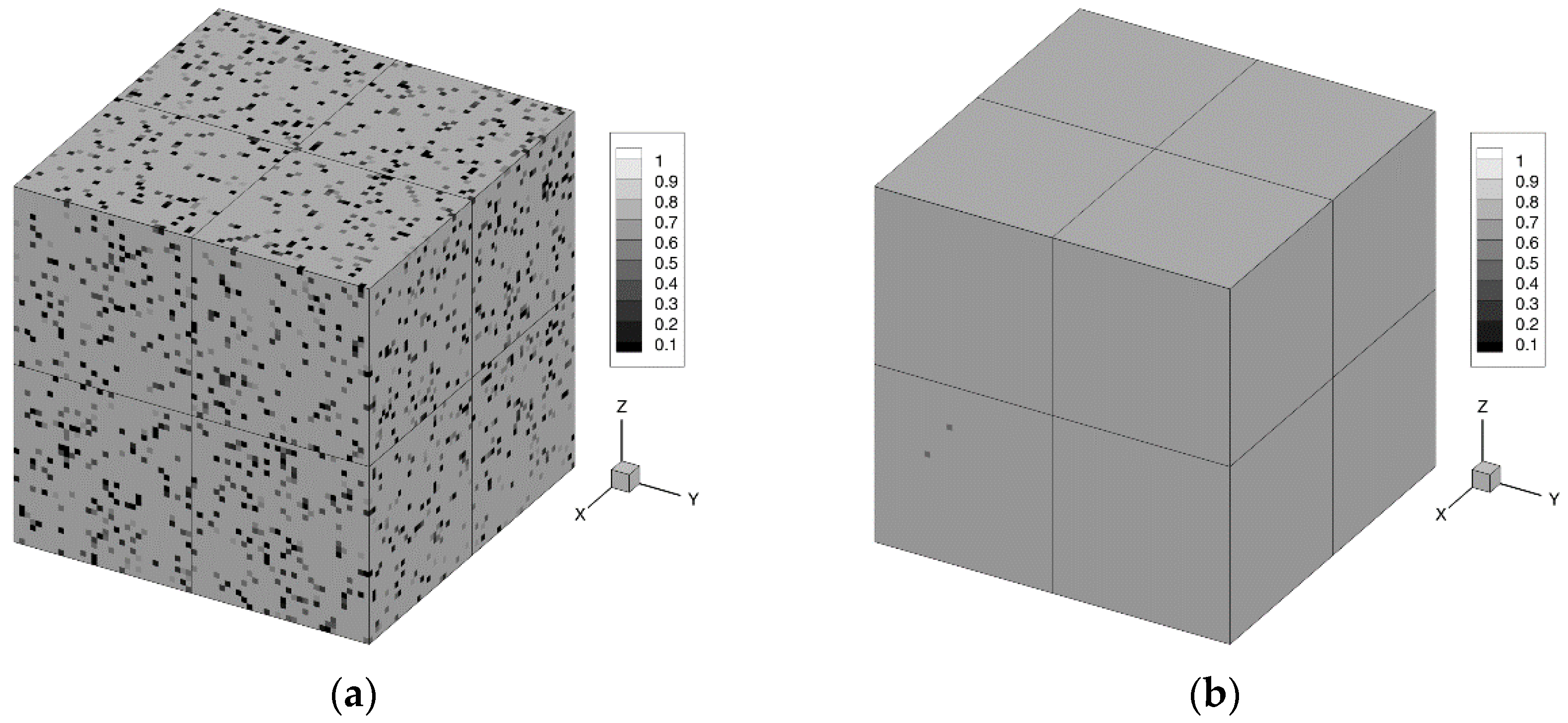
4.1. Consistent Initial Field Problem

The problem of specifying the initial fields of the subgrid-scale turbulence parameters consistent with the resolved flow field is described in [13,16]. In [13], use of the Smagorinsky model is proposed [3] to determine the turbulent viscosity at each cell of the computational domain. Further, the subgrid-scale kinetic energy, k, is proposed to be considered as the difference between the total turbulence energy (obtained theoretically by integrating the one-dimensional spectrum provided from the Comte-Bellot and Corrsin experiment [30,31] over the whole wavenumber range) and the kinetic energy of the resolved scales. After that, the characteristic subgrid-scale frequency value $\omega$ can be estimated as $\omega =k/{\nu }_t$. In our viewpoint, this method is relatively laborious. Moreover, it is worth noting that the procedure of obtaining a consistent initial field must be applied to all unsteady flows. This means that a more general approach is needed (especially in cases when total turbulence energy is unknown). In this paper, an original method based on [16] was used. To obtain the initial field, only the equations for the subgrid-scale turbulence parameters were solved (none of the rest of the flow parameters changed during the simulation); the fields of these parameters trended toward a stationary state consistent with the resolved velocity field obtained from the turbulence generator. However, the convergence algorithm was simplified; the approach to the stationary state was tracked using the subgrid-scale kinetic energy averaged over the computational domain. The $\omega$ field relaxation was not tracked, since it was found to reach a stationary state several times more quickly than did the $k$ field. Figure 2 shows the dependence of the volume-averaged subgrid-scale kinetic energy, $k_{ave}$, on physical time with use of a central-difference scheme and the standard value $C_{DES2}=0.61$ (see Section 1) on a mesh of 64³ cells. The value $k_{ave}$ was seen to significantly change during the first integral time scale, $t\le T_0\approx 0.06$ s. By the time equal to $2T_0\approx 0.12$ s, the $k_{ave}$ value had almost stopped changing (changes occurred in the fifth significant digit). A similar behavior was observed for other $C_{DES2}$ values on the same mesh. As a result, it was decided to carry out this procedure up to a time equal to $3T_0\approx 0.18$ s, assuming that for this time period on any of the considered meshes and for any values of the subgrid-scale parameter field, there would be enough time to adjust to the initial resolved field. At the same time, each value of the $C_{DES2}$ constant corresponds to its own established value, $k_{ave}$.

Another observation that can be made from Figure 2 is that the initial subgrid turbulent energy with $C_{DES2}=0.61$ took on a value of about 11% of the resolved turbulent energy. This corresponds to a relation that is typical for LES [32].

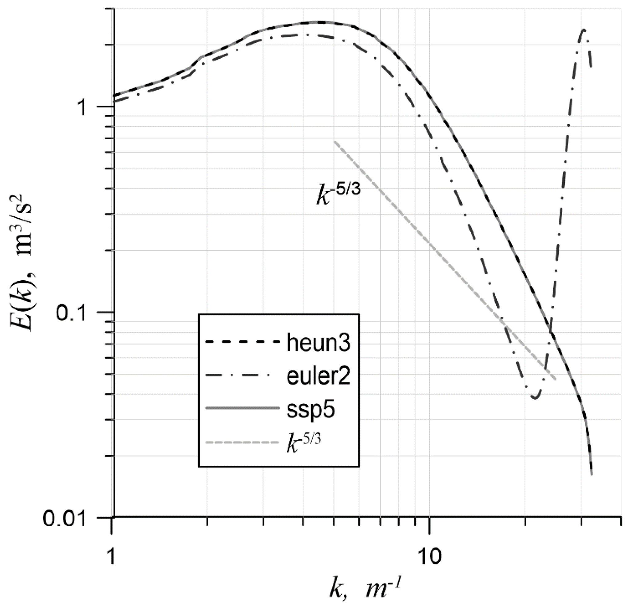
4.2. Choice of Temporal Approximation

The first series of simulations was devoted to a comparison and the choice of a temporal approximation. For this, a mesh with 64 cells in each direction and the value of $C_{DES2}=1$ (value 1 was found to be optimal in [16]) were used, and convective fluxes were approximated with CD-4. All three of the time schemes mentioned in Section 2 were considered. The time step did not exceed $8\times {10}^{-5}$ s. in any case. Figure 3 shows the energy spectra for these schemes at the end of each simulation. The euler2 scheme was seen to create an overshoot of energy in the short-wavelength spectrum region. Thus, it is less stable within the framework of the test problem in comparison with the other two schemes. The heun3 and ssp5 schemes made it possible to obtain identical spectrum shapes, which indicates a negligible contribution of their residual terms to the equations’ balance. This means that the heun3 scheme is sufficient for further simulations. We noted an additional benefit of the heun3 scheme compared to ssp5: it has three intermediate stages at each step rather than five. As a result, it is possible to advance in time more efficiently. Another conclusion that can be drawn from Figure 3 is that the chosen preliminary value of the constant $C_{DES2}=1$ turned out to be too high; the inertial interval $k^{-5/3}$ was not maintained in the spectra.

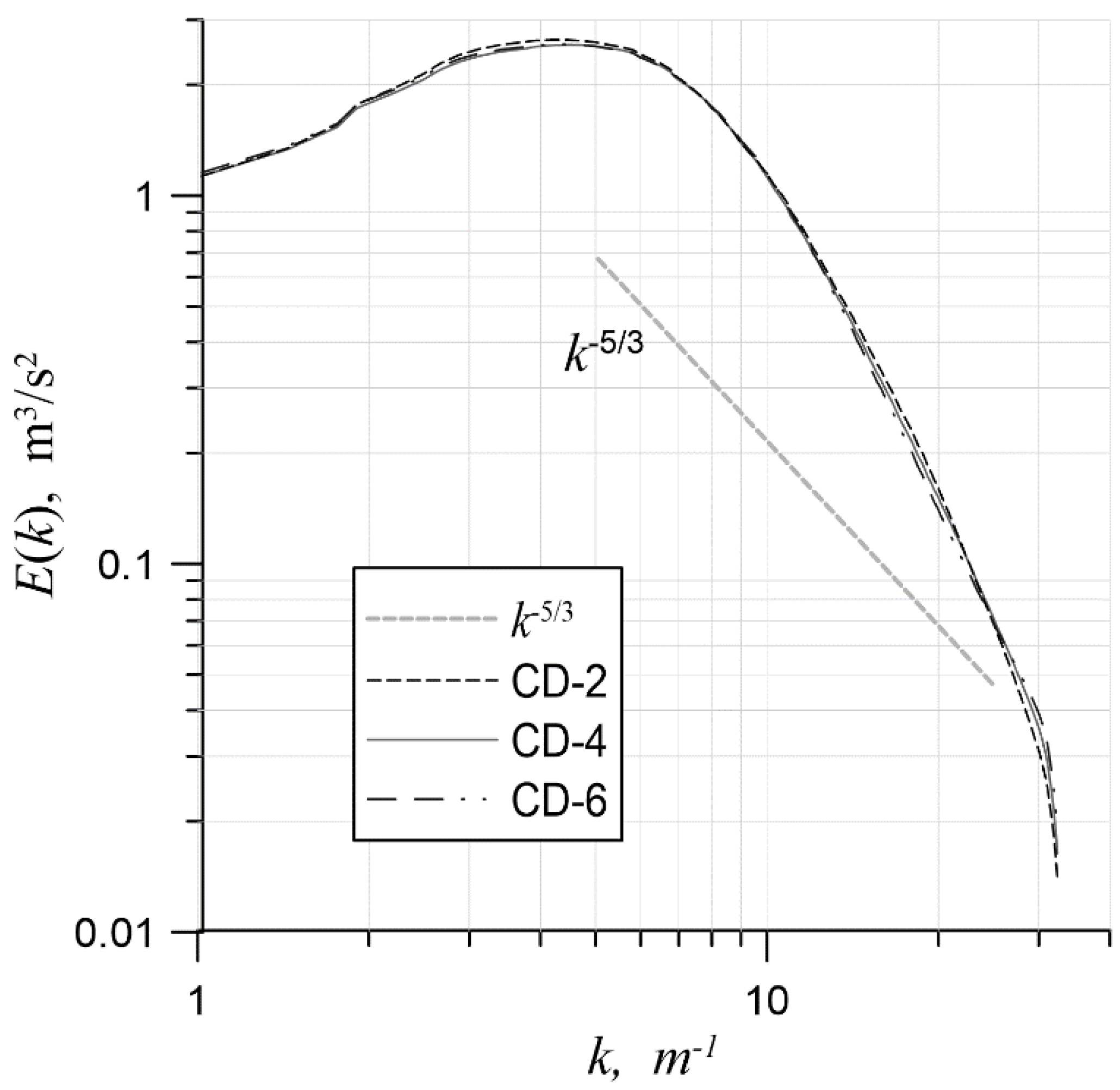
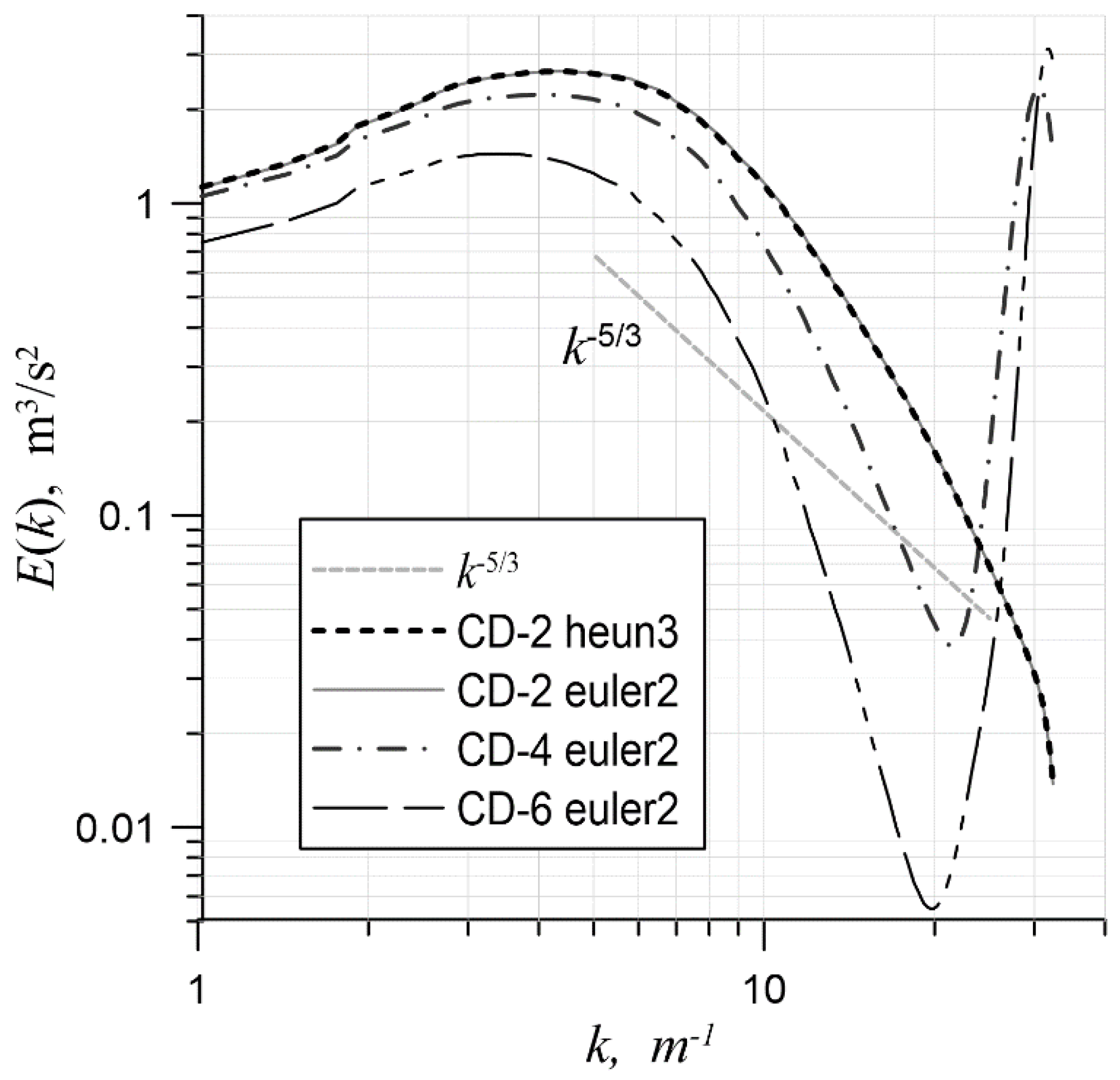
4.3. Choice of Central Differences

In the second series of simulations, the central-difference scheme was varied, with a fixed heun3 time scheme (Figure 4). Interestingly, all three of the central-difference schemes gave similar results. This was probably due to the fact that solution reconstruction was carried out independently along the mesh directions and one quadrature point was taken on each face. This led to a restriction on the order of the scheme when equations were solved in a multidimensional case. It should also be noted that when the euler2 time scheme was used, simulations with spatial approximations CD-2, CD-4 and CD-6 gave significantly different results (Figure 5).

It turns out that with an increase in the order of the central-difference scheme, its stability decreases. This can also be demonstrated using the convection equation $u_t+c\cdot u_x=0$, where c is speed of convection, with the help of the von Neumann stability analysis. It is convenient to represent the solution at the j-th cell on the n-th time layer in the spectral form: $u_j^n={\lambda }^n\cdot e^{ij\alpha }$, where $e^{ij\alpha }$ is an eigenfunction of the numerical operator of transition to a new time layer and $\lambda$ is an eigenvalue. The necessary condition for stability has the following form: $\underset{{}^{\lambda }}{\max }\left|\lambda \right|\le 1+O(\tau )$ when $\tau ,h\to 0$. In consideration of the euler2 time scheme, it is possible in the case of CD-2 to substitute approximations and express $u_j^{n+1}$:

$$u_j^{n+1}=u_j^n-\frac{c\tau }{2h}\left[u_{j+1}^n-u_{j-1}^n-\frac{c\tau }{4h}\left(u_{j+2}^n+u_{j-2}^n-2u_j^n\right)\right].$$

Therefore,

$$\lambda =1-\frac{c\tau }{2h}\left[e^{i\alpha }-e^{-i\alpha }-\frac{c\tau }{4h}\left(e^{2i\alpha }+e^{-2i\alpha }-2\right)\right]=1-\frac{c\tau }{2h}\left[2i\sin \alpha +\frac{c\tau }{h}{\sin }^2\alpha \right],$$

From which it follows that

$$\left|\lambda \right|=\sqrt{{\left(1-\frac{1}{2}{\left(\frac{c\tau \sin \alpha }{h}\right)}^2\right)}^2+{\left(\frac{c\tau \sin \alpha }{h}\right)}^2}=\sqrt{1+\frac{1}{4}{\left(\frac{c\tau \sin \alpha }{h}\right)}^4}.$$

Obviously, $\max \left|\lambda \right|=\sqrt{1+\frac{1}{4}{c}^{4}r\tau }\le 1+\frac{c^{4}r}{8}\tau$ when $\tau =r^{1/3}{h}^{4/3}$; r is a dimensional constant coefficient. This means that the scheme is conditionally stable [33]. The following can be similarly obtained for CD-4: $\max \left|\lambda \right|=\sqrt{1+\frac{64}{81}{\left(\frac{c\tau }{h}\right)}^4}=\sqrt{1+\frac{64}{81}{c}^{4}r\tau }\le 1+\frac{32c^{4}r}{81}\tau$. Thus, in the spectral plane, the set of points that correspond to the growing solution amplitude of CD-2 scheme is within the corresponding set of the CD-4 scheme. This means that in the case of CD-4, bigger harmonics can appear at each time step. Through use of the heun3 scheme for CD-2, it is possible to obtain the following:

$$\begin{gathered} \left|\lambda \right|=\sqrt{{\left(1-\frac{1}{2}{\left(\frac{c\tau \sin \alpha }{h}\right)}^2\right)}^2+{\left(\frac{c\tau \sin \alpha }{h}-\frac{1}{6}{\left(\frac{c\tau \sin \alpha }{h}\right)}^3\right)}^2} \\ =\sqrt{1+\frac{1}{36}{\left(\frac{c\tau \sin \alpha }{h}\right)}^4\cdot \left[{\left(\frac{c\tau \sin \alpha }{h}\right)}^2-3\right]}. \end{gathered}$$

The value of $\left|\lambda \right|$ reaches a maximum when $\sin \alpha =1$. In this case, it is possible to obtain a stronger stability condition: $\left|\lambda \right|<1$. To attain this, it is necessary for the right factor of the radicand to be less than or equal to 0: ${\left(\frac{c\tau }{h}\right)}^2-3\le 0$. Therefore, the scheme is conditionally stable at $\tau \le \frac{\sqrt{3}}{c}h$. Interestingly, the relationship between the time step, $\tau$, and the mesh spacing, $h$, turned out to be linear here (the linear dependence that is used in solving practical problems, including the problem of isotropic turbulence decay). In the case of CD-4 and the heun3 scheme, it is possible to write the expression for $\left|\lambda \right|$ as follows:

$$\left|\lambda \right|=\sqrt{1+{\left(\frac{c\tau }{3h}(4-\cos \alpha )\sin \alpha \right)}^4\frac{1}{36}\left[{\left(\frac{c\tau }{3h}(4-\cos \alpha )\sin \alpha \right)}^2-3\right]}.$$

The expression in the second set of parentheses attains its maximum at $\cos \alpha =1-\sqrt{3/2}$. The stability condition may be expressed as: $\tau \le 3\sqrt{\frac{12}{\xi }}\frac{h}{c},$ where $\xi =4\left(2\sqrt{\frac{3}{2}}-\frac{3}{2}\right)\cdot {\left(3+\sqrt{\frac{3}{2}}\right)}^2\approx 67.79$. Therefore, the limit on $\tau$ is approximately $1.26\frac{h}{c}$. As a result, CD-4 has a stricter stability condition than CD-2.

In Figure 5, it can be seen that only in the case of CD-2, the spectrum obtained using the euler2 scheme is similar to the spectra obtained using other temporal approximations. However, the more accurate spatial schemes were observed to suffer from the effect of energy pumping in the short-wavelength region. With this taken into account, the CD-2 scheme was chosen for all further simulations. The heun3 scheme was chosen as a temporal approximation, since in the case of the convection equation, unlike the Euler methods, it is stable when $\tau$ and $h$ are linearly related and when central-difference spatial approximations are used.

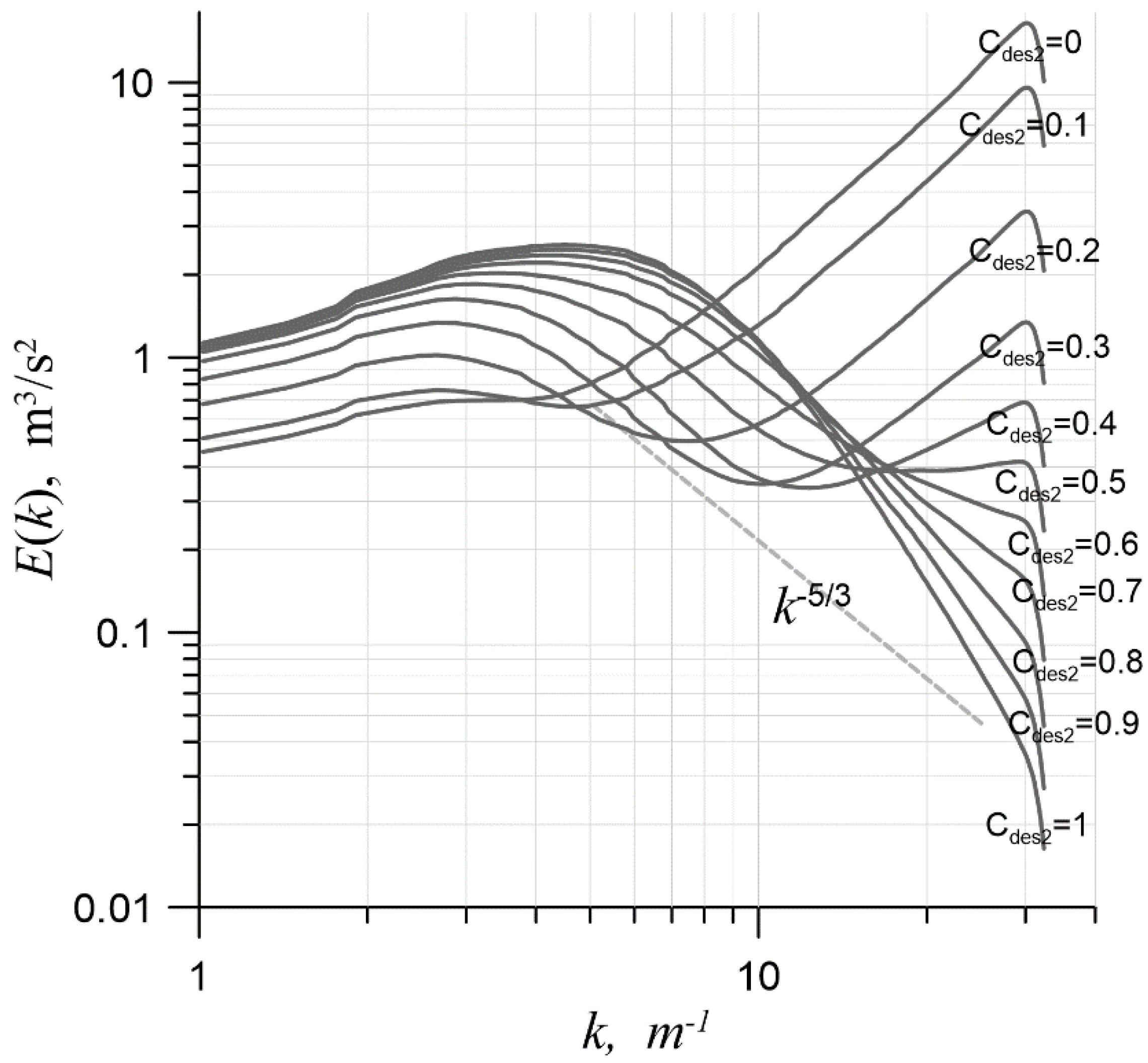
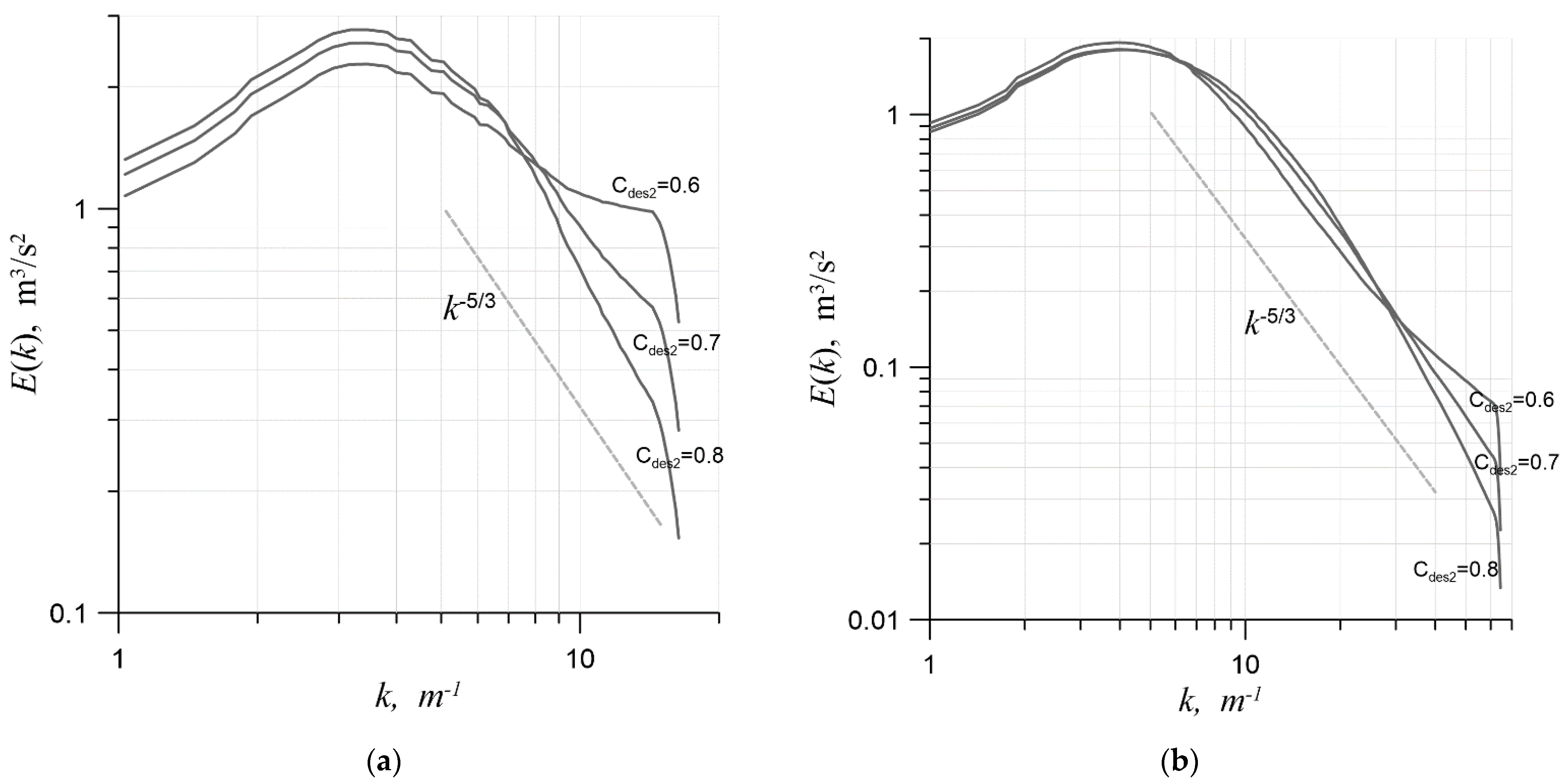
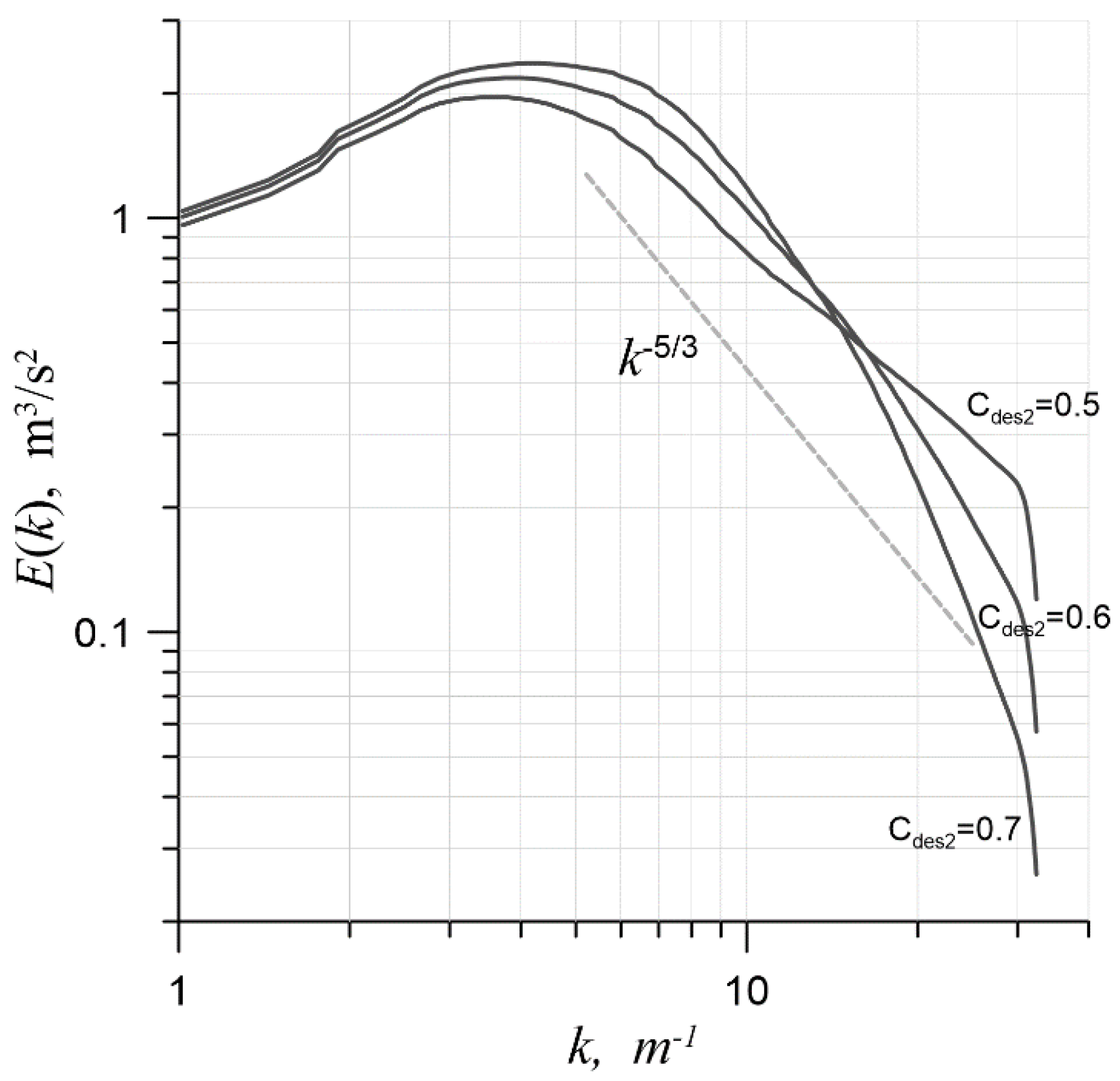
4.4. Constant Calibration

The third series of simulations was devoted to the calibration of the subgrid model constant $C_{DES2}$ while using the previously chosen CD-2 central-difference scheme and the heun3 temporal approximation. The method for choosing the optimal value of $C_{DES2}$ is described below. A series of simulations was carried out with different values of the constant, ranging from 0 to 1 with a step of 0.1. After that, a power-law range was found on the energy spectrum graph, and the exponent $E\left(k\right)~k^{\alpha }$ was determined for it. Then, an error function, $\epsilon$, was introduced as the difference between the exponent and the theoretical value $-5/3$. If the condition $\left|\epsilon \right|<0.01$ was satisfied for some of the spectra, then the corresponding value of the constant $C_{DES2}$ would be declared optimal. Otherwise, a parabola would be constructed from the three values of $\epsilon$ closest to 0, depending on $C_{DES2}$. Furthermore, the point at which the parabola took on a value of zero was declared optimal, and an additional simulation was carried out with a new value of $C_{DES2}$.

Figure 6 shows the spectra obtained at various values of $C_{DES2}$ on a mesh with 64³ cells. It can be seen that as $C_{DES2}$ increased, the level of dissipation in the short-wavelength region of the spectrum became larger due to growing influence of the subgrid model. Visually, the theoretical slope corresponded to values $C_{DES2}=0.7$ and $0.8$; however, according to the method described above, for both cases, the error exceeded the specified threshold of $0.01$. As a result of a parabolic interpolation, the optimal value of $C_{DES2}$ turned out to be $0.69$. It is worth noting that in [16], the optimal value of the constant was equal to $1.2$. This difference can be explained by the fact that VTM averaging was not used in [16] (Figure 1). This led to a decrease in the value of $\Delta$ in a certain set of cells; this was compensated by an increase in $C_{DES2}$. It is worth noting that regardless of the local VTM averaging, the global average values over the computational domain were close to 1: $\overline{F_{KH}(\mathrm{VTM})}\approx 0.930$ and $\overline{F_{KH}(<\mathrm{VTM}>)}\approx 0.999$. Meanwhile, the optimal values of the constants differed by a factor of 1.7.

Figure 7a shows the spectra closest to optimal on a mesh with 32³ cells; they correspond to the values $C_{DES2}=0.6$, $0.7$ and $0.8$. A similar result is shown in Figure 7b for a mesh with 128³ cells. On the coarse mesh, the optimal value turned out to be $0.70$, and on the most refined mesh, it was $0.68$. The optimal value of $C_{DES2}$ barely depended on mesh spacing, which is a good sign that the methods were used within their ranges of applicability in this problem; therefore, the obtained values of the coefficient can be trusted.

Figure 8 shows the energy spectrum obtained in the simulation with the use of the CD-2 scheme with the optimal value of the coefficient $C_{DES2}=0.69$ (solid line). The extended inertial interval is clearly visible almost up to the cutoff wavenumber, $k_{cut}$ (for the given mesh, $k_{cut}=32$).

$C_{DES2}$ calibration was also carried out for the above-described hybrid scheme (as before, the heun3 scheme was used as the temporal approximation). Figure 9 shows the spectra on a mesh with 64³ cells at $C_{DES2}=0.5$, $0.6$ and $0.7$. The optimal value of $C_{DES2}$ in the presence of upwind approximations turned out to be smaller than that of a pure central-difference scheme: namely, 0.56. The spectrum obtained with this value of the constant in the case of a hybrid scheme is shown in Figure 8 (dashed line). The inertial interval was as wide as it would have been in the case of a pure central-difference approximation (solid curve, Figure 8), although a slight upward convexity could be seen upon closer consideration. Despite this remark, the hybrid scheme is of the most interest for practical simulations. Indeed, in the presence of RANS regions and non-turbulent regions far from the domain of study, switching to the upwind scheme is a necessary condition for stable simulation [23].

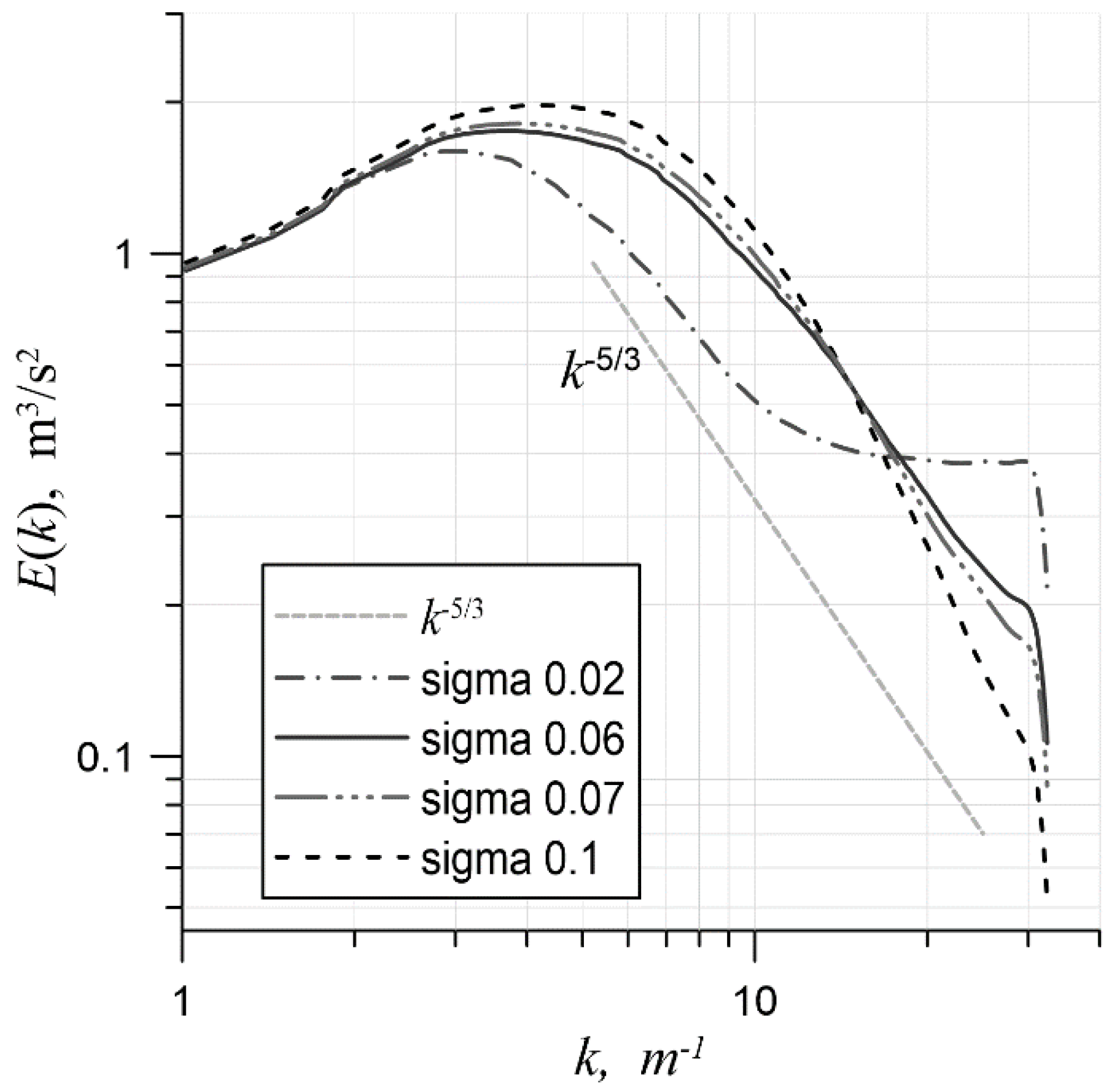
4.5. Determining the Maximum Weight of the Upwind Scheme

In the final series of simulations, a numerical experiment was carried out. Its task was to determine the maximum constant weight of the upwind scheme at which the influence of the explicit subgrid model was still present in the solution. The practical interest of this experiment was that the critical value of the upwind scheme weight, $\sigma *$, would be determined. For all values over $\sigma *$, it would be possible to conduct an LES using a more economical ILES (implicit large eddy simulation) method without the risk of energy pumping in the short-wavelength region.

This problem was reduced to finding a constant weight, $\sigma *$, at which the simulation where $C_{DES2}=0$ would make it possible to obtain a solution with a sufficiently small error in the power law $E\left(k\right)~k^{-5/3}$ on the inertial interval. Simulations were carried out on a mesh with 64³ cells. Formally, the subgrid model was included, but taking $C_{DES2}$ to be equal to ${10}^{-3}$ resulted in the model working in ILES mode.

Figure 10 shows the spectra for several different $\sigma$ values. At $\sigma =0.02$, an energy overshoot can still be seen in the short-wavelength region of the spectrum, and at $\sigma =0.1$, the scheme had already turned out to be excessively dissipative. Simulations with values of $\sigma$ equal to 0.06 and 0.07 were close to the correct slope of the spectrum. The fact that the threshold value turned out to be very small ($\sigma *\in \left[0.06,0.07\right]$) suggests that the optimal values of $C_{DES2}$ obtained above are relevant only to those schemes whose behavior is very close to that of the central difference. When the approximation of the convective term reaches 6–7 percent of the upwind scheme, the coefficient $C_{DES2}$ in the simulation should be assumed to be equal to 0.

5. Conclusions

Hybrid upwind-central spatial approximations and time-integration schemes were analyzed and optimized for a modern version of detached eddy simulation: namely, SST-DDES. A method for selecting the appropriate level of subgrid viscosity was proposed. A series of LES simulations of homogeneous isotropic turbulence decay was carried out. The issue of generating a consistent initial field of subgrid variables was considered. The conducted research led to the following conclusions:

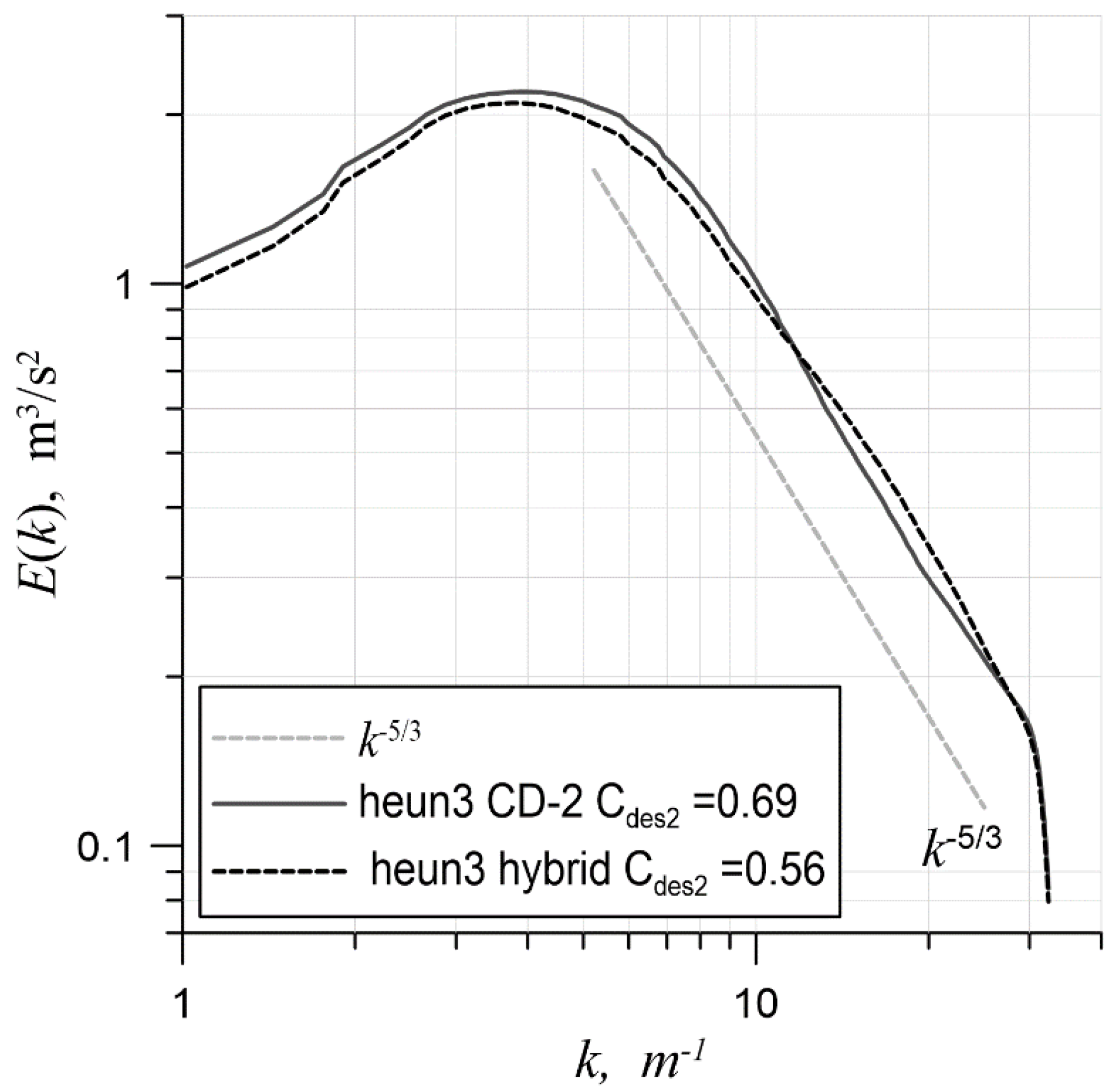
• Firstly, for simulations using the current implementation of DDES in zFlare, a hybrid scheme based on a central-difference scheme of the second order of accuracy and the explicit three-step Heun method (which has a weaker time-step constraint than the midpoint method) is recommended to maximize computational efficiency, at least if the computational mesh is close to uniform;
• Secondly, with the recommended hybrid numerical method, the optimal value of $C_{DES2}$ was found to be 0.56. This value was almost independent of the mesh spacing, at least if its cutoff scale fell within the inertial interval. At the same time, the optimal value of $C_{DES2}$ for a pure central-difference scheme of the second order of accuracy equal to 0.69 was found;
• Thirdly, the influence of the subgrid model very quickly decreased with an increase in the weight of the upwind part of the numerical scheme. It became insignificant at values as low as $\sigma =0.07$, which indicates a possibility of using these schemes with the ILES method in eddy-resolving regions.

References

1. Spalart, P.R. Strategies for turbulence modelling and simulations. Int. J. Heat Fluid Flow 2000, 21, 252–263. [Google Scholar] [CrossRef]
2. Reynolds, O. On the Dynamical Theory of Incompressible Viscous Fluids and the Determination of the Criterion. Phil. Trans. R. Soc. Lond. 1895, 186, 123–164. [Google Scholar]
3. Smagorinsky, J. General circulation experiments with the primitive equations: I. The basic experiment. Mon. Weather. Rev. 1963, 91, 99–164. [Google Scholar] [CrossRef]
4. Lilly, D.K. The Representation of Small-Scale Turbulence in Numerical Simulation Experiments; IBM Form: Yorktown Heights, NY, USA, 1967; pp. 195–210. [Google Scholar]
5. Deardorff, J.W. A numerical study of three-dimensional turbulent channel flow at large Reynolds numbers. J. Fluid Mech. 1970, 41, 453–480. [Google Scholar] [CrossRef]
6. Kolmogorov, A.N. The local structure of turbulence in incompressible viscous fluid for very large Reynolds numbers. CR Acad. Sci. USSR 1941, 30, 301–305. [Google Scholar]
7. Chaouat, B. The state of the art of hybrid RANS/LES modeling for the simulation of turbulent flows. Flow Turbul. Combust. 2017, 99, 279–327. [Google Scholar] [CrossRef] [Green Version]
8. Shur, M.; Spalart, P.R.; Strelets, M.; Travin, A. Detached-eddy simulation of an airfoil at high angle of attack. In Engineering Turbulence Modelling and Experiments 4; Elsevier Science Ltd.: Amsterdam, The Netherlands, 1999; pp. 669–678. [Google Scholar] [CrossRef]
9. Spalart, P.R.; Deck, S.; Shur, M.L.; Squires, K.D.; Strelets, M.K.; Travin, A. A new version of detached-eddy simulation, resistant to ambiguous grid densities. Theor. Comput. Fluid Dyn. 2006, 20, 181–195. [Google Scholar] [CrossRef]
10. Travin, A.; Shur, M.; Strelets, M.; Spalart, P.R. Physical and Numerical Upgrades in the Detached-Eddy Simulation of Complex Turbulent Flows. Fluid Mech. Appl. 2002, 65, 239–254. [Google Scholar] [CrossRef]
11. Gritskevich, M.S.; Garbaruk, A.V.; Schütze, J.; Menter, F.R. Development of DDES and IDDES Formulations for the k-ω Shear Stress Transport Model. Flow Turbul. Combust. 2012, 88, 431–449. [Google Scholar] [CrossRef]
12. Yu, H.; Grimaji, S.S.; Luo, L.S. DNS and LES of decaying isotropic turbulence with and without frame rotation using lattice Boltzmann. J. Comp. Phys. 2005, 209, 599–616. [Google Scholar] [CrossRef]
13. Hansen, A.; Sørensen, N.N.; Johansen, J.; Michelsen, J.A. Detached-eddy simulation of decaying homogeneous isotropic turbulence. In Proceedings of the 43rd AIAA Aerospace Sciences Meeting and Exhibit 2005, Reno, NV, USA, 10–13 January 2005; p. 885. [Google Scholar] [CrossRef]
14. Chumakov, S.G.; Rutland, C.J. Dynamic structure subgrid-scale models for large eddy simulation. Int. J. Numer. Methods Fluids 2005, 47, 911–923. [Google Scholar] [CrossRef]
15. Zhou, Z.; He, G.; Wang, S.; Jin, G. Subgrid-scale model for large-eddy simulation of isotropic turbulent flows using an artificial neural network. Comput. Fluids 2019, 195, 104319. [Google Scholar] [CrossRef] [Green Version]
16. Bakhne, S. Comparison of convective terms’ approximations in DES family methods. Math. Model. Comput. Sim. 2022, 14, 99–109. [Google Scholar] [CrossRef]
17. Bakhne, S.; Bosniakov, S.M.; Mikhailov, S.V.; Troshin, A.I. Comparison of gradient approximation methods in schemes designed for scale-resolving simulations. Math. Model. Comput. Sim. 2020, 12, 357–367. [Google Scholar] [CrossRef]
18. Troshin, A.; Bakhne, S.; Sabelnikov, V. Numerical and physical aspects of large-eddy simulation of turbulent mixing in a helium-air supersonic co-flowing jet. In Progress in Turbulence IX; Örlü, R., Talamelli, A., Peinke, J., Oberlack, M., Eds.; Springer: Berlin/Heidelberg, Germany, 2021; pp. 297–302. [Google Scholar] [CrossRef]
19. Bosnyakov, S.; Kursakov, I.; Lysenkov, A.; Matyash, S.; Mikhailov, S.; Vlasenko, V.; Quest, J. Computational tools for supporting the testing of civil aircraft configurations in wind tunnels. Prog. Aerosp. Sci. 2008, 44, 67–120. [Google Scholar] [CrossRef]
20. Zhang, R.; Zhang, M.; Shu, C.W. On the order of accuracy and numerical performance of two classes of finite volume WENO schemes. Commun. Comput. Phys. 2011, 9, 807–827. [Google Scholar] [CrossRef] [Green Version]
21. Suresh, A.; Huynh, H. Accurate Monotonicity-Preserving Schemes with Runge–Kutta Time Stepping. J. Comput. Phys. 1997, 136, 83–99. [Google Scholar] [CrossRef] [Green Version]
22. Godunov, S.K.; Zabrodin, A.V.; Ivanov, M.I.; Kraiko, A.N.; Prokopov, G.P. Numerical Solution of Multidimensional Problems of Gas Dynamics; Nauka: Moscow, Russia, 1976; p. 400. [Google Scholar]
23. Guseva, E.K.; Garbaruk, A.V.; Strelets, M.K. An automatic hybrid numerical scheme for global RANS-LES approaches. J. Phys. Conf. Ser. 2017, 929, 83–99. [Google Scholar] [CrossRef] [Green Version]
24. Fornberg, B. Generation of Finite Difference Formulas on Arbitrarily Spaced Grids. Math. Comput. 1988, 51, 699–706. [Google Scholar] [CrossRef]
25. van Leer, B.; Lee, W.T.; Roe, P.L.; Powell, K.G.; Tai, C.H. Design of Optimally Smoothing Multistage Schemes for the Euler Equations. Commun. Appl. Numer. Methods 1992, 8, 761–769. [Google Scholar] [CrossRef] [Green Version]
26. Shur, M.L.; Spalart, P.R.; Strelets, M.K.; Travin, A.K. An Enhanced Version of DES with Rapid Transition from RANS to LES in Separated Flows. Flow Turbul. Combust. 2015, 95, 709–737. [Google Scholar] [CrossRef]
27. Batchelor, G.K. The Theory of Homogeneous Turbulence; Cambridge University Press: Cambridge, UK, 1953; 197p. [Google Scholar]
28. Shur, M.L.; Spalart, P.R.; Strelets, M.K.; Travin, A.K. Synthetic Turbulence Generators for RANS-LES Interfaces in Zonal Simulations of Aerodynamic and Aeroacoustic Problems. Flow Turbul. Combust. 2014, 93, 63–92. [Google Scholar] [CrossRef]
29. Etkin, B. Dynamics of Atmospheric Flight; John Wiley & Sons, Inc.: New York, NY, USA, 1972; 340p. [Google Scholar]
30. Comte-Bellot, G.; Corrsin, S. The use of a contraction to improve the isotropy of grid-generated turbulence. J. Fluid Mech. 1966, 25, 657–682. [Google Scholar] [CrossRef]
31. Comte-Bellot, G.; Corrsin, S. Simple Eulerian time correlation of full- and narrow-band velocity signals in grid-generated, ‘isotropic’ turbulence. J. Fluid Mech. 1971, 48, 273–337. [Google Scholar] [CrossRef]
32. Sagaut, P. Large Eddy Simulation for Incompressible Flows: An Introduction, 3rd ed.; Springer Science & Business Media: Berlin/Heidelberg, Germany, 2006. [Google Scholar]
33. Godunov, S.K.; Ryabenkii, V.S. Difference Schemes an Introduction to the Underlying Theory; Elsevier Science Publ.: Amsterdam, The Netherlands, 1987; 490p. [Google Scholar]
Figure 1. The field of the weight, F K H ( VTM ) , on mesh with 643 cells. (a) Without VTM averaging; (b) with VTM averaging.
Fluids 07 00376 g001
Figure 2. The evolution of k a v e with C D E S 2 = 0.61 on the mesh with 643 cells.
Fluids 07 00376 g002
Figure 3. The turbulent-energy spectrum for three different time schemes on the mesh with 643 cells; C D E S 2 = 1 .
Fluids 07 00376 g003
Figure 4. The energy spectrum for various central-difference approximations on a mesh with 643 cells and heun3; C D E S 2 = 1 .
Fluids 07 00376 g004
Figure 5. The energy spectrum for various central-difference approximations on a mesh with 643 cells and euler2; C D E S 2 = 1 .
Fluids 07 00376 g005
Figure 6. The spectrum on a mesh with 643 cells, with different C D E S 2 values.
Fluids 07 00376 g006
Figure 7. The energy spectrum with different C D E S 2 values: (a) on a mesh with 323 cells and (b) on a mesh with 1283 cells.
Fluids 07 00376 g007
Figure 8. The energy spectra at optimal values of C D E S 2 (0.69 for CD-2 and 0.56 for the hybrid scheme) on a mesh with 643 cells.
Fluids 07 00376 g008
Figure 9. The energy spectra on a mesh with 643 cells at different values (0.5, 0.6, 0.7) using a hybrid scheme.
Fluids 07 00376 g009
Figure 10. The energy spectra in a series of ILES at various constant values of σ on a mesh with 643 cells.
Fluids 07 00376 g010
Publisher’s Note: MDPI stays neutral with regard to jurisdictional claims in published maps and institutional affiliations.