Article

CFD Investigation into the Effects of Surrounding Particle Location on the Drag Coefficient

1
Department of Mechanical and Product Design Engineering, Swinburne University of Technology, Hawthorn, VIC 3122, Australia
2
Department of Biomedical Engineering, The University of Melbourne, Carlton, VIC 3010, Australia
*
Author to whom correspondence should be addressed.
Fluids 2022, 7(10), 331; https://doi.org/10.3390/fluids7100331
Submission received: 10 September 2022 / Revised: 10 October 2022 / Accepted: 13 October 2022 / Published: 17 October 2022
(This article belongs to the Special Issue Recent Advances in Fluid Mechanics: Feature Papers, 2022)

Abstract

:
In the simulation of dilute gas-solid flows such as those seen in many industrial applications, the Lagrangian Particle Tracking method is used to track packets of individual particles through a converged fluid field. In the tracking of these particles, the most dominant forces acting upon the particles are those of gravity and drag. In order to accurately predict particle motion, the determination of the aforementioned forces become of the upmost importance, and hence an improved drag force formula was developed to incorporate the effects of particle concentration and particle Reynolds number. The present CFD study examines the individual effects of particles located both perpendicular and parallel to the flow direction, as well as the effect of a particle entrain within an infinite matrix of evenly distributed particles. Results show that neighbouring particles perpendicular to the flow (Model 2) have an effect of increasing the drag force at close separation distances, but this becomes negligible between 5–10 particle diameters depending on particle Reynolds number (Rep). When entrained in an infinite line of particles co-aligned with the flow (Model 1), the drag force is remarkably reduced at close separation distances and increases as the distance increases. The results of the infinite matrix of particles (Model 3) show that, although not apparent in the individual model, the effect of side particles is experienced many particle diameters downstream.

1. Introduction

Dilute gas-solid flows are of considerable importance in many technical and industrial processes to efficiently transport solid particles that have a wide range of sizes (few µm to few mm) and density [1,2]. The application includes, but not limited to pneumatic conveying, fluidised beds, vertical risers, classifiers, cyclones, and flow mixing devices [3,4]. Pneumatic conveying, due to its many advantages such as simplicity and flexibility in operation, environmental compliance, and inherent safety, is widely used in the chemical, food processing, and cement industries and also in order to transport pulverised coal in thermal power plants [5]. This wide application has led to extensive research on pneumatic conveying of solids through the different pipe elements [6,7]. Despite its wide application, the design of the pipe network for pneumatic conveying is still a challenge because ostensibly small changes in the system or product frequently cause significant changes in the system performance or design [8]. Furthermore, during the flowing, these fine particles have not only the interactions with gas phase but also the collisions with each other and the wall of the pipes [9,10]. Therefore, the flow phenomena of gas–solid two-phase flows are very complex. Computational Fluid Dynamics (CFD) is usually used for modelling the flow in these systems for a number reasons ranging from the design stage to monitoring flows where experimental measurements are unavailable.
The CFD modelling relies heavily on a strong knowledge base of the fluid flow under consideration, and as such, the behaviour of particle motion is of the utmost importance when trying to simulate gas particle flows [11]. Over the years, many researchers have looked into the CFD modelling of gas-particle flows and the degree of accuracy has greatly improved with advances in turbulence modelling and computing power [12,13,14]. In many applications, the importance of the drag force in accurately predicting particle motion cannot be understated [15,16]. When looking at gas driven flows, the drag force is responsible for the acceleration of the particles. In CFD simulations, especially using the Lagrangian framework [17], the most common approach to determine the drag force on a particle is using the standard drag coefficient curve, which is based on experimental studies of a sphere in unbounded fluid flow. The most commonly accepted approximation of this curve is given by the following equation [18]:
C D = 24 Re 1 + 0.15 Re 0.687 Re < 1000
As it can be seen, the above equation is solely a function of the local particle Reynolds number, and as such, discounts other effects that may affect the drag on a particle. In a situation whereby particles are relatively spread out, this assumption can be correctly employed to accurately predict particle motion, but in many industrial flows, it is impossible to assume that the distribution will be such that particles will not interact and in turn will affect each other’s motion.
A number of researchers have tried to measure the influence on the drag force of a particle in the presence of other particles. Liang, Hong and Fan [19] proved that altering the position of surrounding particles experienced drastic changes in drag coefficient. A configuration of three-coaligned particles led to a reduction of drag experienced by the centre particle compared with that of the leading particle at a separation distance of 2–3 dp. Cheng and Papanicolaou [20] calculated the analytical force on an array of particles at low Reynolds numbers and volume fraction. The analytical results showed good comparison with the phenomenological results available at the time of this work. Kim, Elghobashi and Sirignano [21] solved the full Navier–Stokes equations for spherical particle motion at a range of Reynolds numbers and particle-to-fluid density ratios. The full Navier–Stokes solution showed considerable differences to some of the more commonly used particle motion formulas and resulted in the authors proposing their own new particle motion formula. Zhang and Fan [16] proposed a new semi analytical expression for the drag force of an interactive particle due to wake effect. This work was based on the experimental findings of Liang, Hong and Fan [19] looking at separation distances up to 7 particle diameters and particle Reynolds number ranging from 54–154. Zhang and Fan [22] used the above work as a basis to predict the rise of interactive bubbles in liquids. The work showed that the new drag model and the inclusion of both the added mass and basset force provided the best agreement with the available experimental data [23].
The work of Liang, Hong and Fan [19] looked at three particles co-aligned and at separation distances up to 7 particle diameters, which corresponds to a particle volume fraction of approximately 10−3. In order to extend this work to investigate the effects at lower concentration values, 10−4, which is common in many dilute phase industrial flows, a full CFD study of this work was undertaken. The aim of this study was to produce a new drag force relation that considered the influence of particle concentration as well as particle Reynolds number. The new relation needed to be a generic equation which relied on the particle concentration or particle volume fraction, α, because the Lagrangian particle tracking method tracks individual representative isolated particles without considering the position of surrounding particles. An assumption was made that because no particle position is actually known, the particles in any given cell are evenly distributed in a cubic formation, see Figure 1. Utilising this assumption, the volume fraction can be transformed into particles separated by a uniform distance in all directions.
ε = V o l u m e o f p a r t i c l e s V o l u m e o f c e l l = 1 6 π d 3 L 3 = π d 3 6 L 3 = π d 3 6 l d 3 = π 6 l 3
where L is the distance between particle centres and l is the distance between particle centres as a ratio of particle diameter.

2. Mathematical Models

This section covers the numerical methods used to solve the motion of both the continuous fluid and the dispersed particle motion. The continuous fluid phase is calculated by solving the governing equations. The dispersed phase is solved in the Lagrangian framework using Newton’s law to describe individual representative particle motion. In present work, CFD technique is used as a tool to develop a new particle drag force equation that considered the influence of particle concentration (α) as well as particle Reynolds number. This paper used the CFX-5 package to replicate experimental work of Liang, Hong and Fan [19].

2.1. Governing Equations

A general form of the transport equation used in CFD model is shown in Equation (3). This equation describes the instantaneous transport of any variable quantity ϕ, which may be mass, momentum, heat, or a scalar quantity such as turbulent kinetic energy.
ρ t ϕ + ρ u i x i ϕ = x i Γ ϕ x i + S
where ρ is the fluid density, x is the distance in the ith, u is the velocity in the ith, Γ is the diffusion coefficient of the variable ϕ and S is a source or sink term for the variable ϕ. For a fluid with constant density, the Navier–Stokes system of equations consist of the continuity Equation (4), derived from the principle of conservation of mass, and three equations derived from the principle of the conservation of momentum (5).
ρ t + x j ρ u i = 0
ρ u i t + ρ u j x j u i = p x i + x j 2 μ s i j
where Sij is the strain tensor, defined as:
s i j = 1 2 u i x j + u j x i

2.2. Turbulence Model

In the present study, the Reynolds Averaged Navier–Stokes (RANS) equation was used to describe turbulent flows. The RANS can be used with approximations based on knowledge of the properties of flow turbulence to give approximate time-averaged solutions to the Navier-Stokes equations. The RANS equation can be written in the following form:
ρ U i t + ρ x j U i U j = p x i + x j 2 μ s i j ρ u i u j ¯
which only differs from the laminar form by the term ρ u i u j ¯ . The quantity is known as the Reynolds stress tensor and has six independent components. As the Reynolds stress tensor contains six unknown quantities combined with the unknown velocity and pressure terms, we now have 10 unknowns and only 4 equations (3 momentum and the continuity) to solve. In order to analytically solve these equations, a form of turbulence closure method is required. The turbulence model used to simulate the experimental results was the standard k-ε model [13]. A Reynolds stress turbulence model was also used in the simulation and compared for accuracy purposes only.

2.3. Particle Phase Model

The calculation of the particle motion comes directly from Newton’s second law, which states:
m d u d t = F
where F is the force on the particle, and m is the mass of the particle. Although this F is made up of a few different forces, the major contributing factor during dilute phase flow is the drag force between the continuum and the dispersed phases.

2.3.1. Drag Force Model

The drag force generally takes the form:
F D = 1 2 A C S ρ C D V Re l V Re l
where A C S is the cross-sectional area perpendicular to the velocity direction, ρ is the density of the continuum medium, V R e l is the relative velocity between the particle and the continuum phase and C D is the coefficient of drag of the particle. The standard model by [24] employed by CFX-5 is given by:
C D = 24 Re 1 + 0.15 Re 0.687
were
Re = ρ V Re l d μ
here d is the diameter of the particle, ρ is the fluid density and μ is the viscosity. This relation for the drag coefficient only relates the amount of drag to the relative velocity. For extremely dilute flows whereby the particles are well dispersed, this relation is adequate, but when the volume fraction of particles increases, the effects of neighbouring particles cannot be excluded. The following section covers the development of a new particle drag coefficient formula considering the effect of neighbouring particles on the drag force particles entrained in particle streams.

2.3.2. Turbulent Dispersion

The effect of the fluid turbulence on the particle motion is considered via the turbulent dispersion method. As the fluid flow is calculated as a time averaged steady-state flow, the velocity at any point can be quantified as a mean and fluctuating component of velocities. The fluctuating components of velocity are calculated using Gaussian probability distribution of zero mean and standard deviation of:
s d = 2 3 k
where k is the kinetic energy of the fluid in a particular cell. This calculated fluctuating component combined with the time-averaged mean value at that point are used to predict particle motion in that immediate area.

2.3.3. Particle-Wall Collision Model

The standard particle-wall collision based of the work of Shuen, Solomon, Zhang and Faeth [25] included in CFX-5 consists of particle being reflected off the wall surface based on the coefficient of restitution. This coefficient is a direct measure of the amount of energy lost during the collision process and effectively reduces the normal velocity of the rebounding particle. The figure shows the relationship between the pre and post collision velocities, both parallel and normal to wall. To model particle wall collision a rough-wall collision model similar to that of Sommerfeld [26] was implemented. This model considers the effects of slight undulations in the wall surface. These slight undulations result in slightly modified impact angles by introducing a virtual wall as seen in Figure 2.
The calculation for post collision velocities is approached the same as normal wall, but the incoming velocities are adjusted to incorporate the slight impact angle change. The formulas to calculate the post-collision velocities for both sliding and non-sliding collisions are as follows:
Non-sliding collision
u 2 = 5 7 u 1
v 2 = e v 1
Sliding collision
u 2 = u 1 + μ d 1 + e v 1
v 2 = e v 1
where u 1 and u 2 represents the corresponding velocities pre and post collision in the tangential direction with respect to the collision, v are the velocities normal to the wall, e is the coefficient of restitution and μ is the coefficient of friction. A non-sliding collision occurs when the following condition is valid:
u 1 7 2 μ o 1 + e v 1
The equations for the standard model and improved are identical, but the incoming velocities for the improved model have been modified according the roughness angle based on the work of [26].

2.3.4. Particle-Particle Collision Model

The standard CFX-5 software [27] package does not account for particle-particle collision as part of the Lagrangian framework. As a consequence, the software needed to be modified to consider the effect of particle collisions through different flow systems. The modelling method implemented into the program is based on the model developed and refined by Sommerfeld [28]. The basis of this method is the creation of a fictitious particle that is used for the calculation of collision probability and if required the collision process.
As the Lagrangian particles are tracked individually through the flow domain, sampling the average particle velocities through a particular computational cell creates a fictitious particle. With the fictitious particle created, the collision probability of collisions occurring between the tracked and fictitious particles is calculated using a similar method for that of the kinetic theory of gases. The formula for the collision probability is as follows:
P c o l l = π 4 D p , r e a l + D p , f i c t 2 u p , r e a l u p , f i c t n p Δ t ,
where D is the diameter of the relevant particle, u the velocity of the relevant particle, n p is the number of particles per unit volume and Δ t is the time step. After the collision probability is calculated, this probability is compared with a random number (RN) that is generated. A collision is to be simulated if the generated RN is less than the P c o l l . When a collision is to be simulated, the location of collision point on the real particle is determined randomly and the resulting post collision velocities calculated using the follows formulas:
u 1 = u 1 1 1 + e 1 + m 1 m 2
where u 1 and u 1 are the pre and post collision velocities, respectively, in the tangential direction relative to the collision vector between particle center at the time of impact, e is the coefficient of restitution between the two particles, and m1 and m2 are the respective masses. In the normal direction, during the collision process, a particle may slide against the wall surface or depending on the friction between the faces, the particle may rotate in a non-sliding collision. The effects of the two sliding conditions are accounted for by:
non-sliding collision
v 1 = v 1 1 2 7 1 + m 1 m 2
sliding collision
v 1 = v 1 1 μ 1 + e u 1 v 1 1 1 + m 1 m 2
where e is the coefficient of restitution, μ is the coefficient of friction and m 1 and m 2 are the respective masses of the considered particles.

3. Numerical Simulation Overview

3.1. Description of the Simulated Cases

The experimental work of Liang, Hong and Fan [19] was used in the present work for numerical method. In their work, four different orientations were investigated. The first considered the effect of varying angle with respect to the flow direction at given separation distance. The second configuration looked a three co-aligned particle in the flow direction. The third test case considered a central test particle surrounded by 6 equally spaced particles in hexagonal configuration. The final case looked at a central test particle surround by 8 particles in cubic orientation. As previously mentioned the three co-aligned particles work forms the basis of the following study whereby separation distances from 0.25 to 7 x/d were investigated where the results for 0–3 x/d were compared with the experimental data of [19]. The published results considered the flow conditions where the particle Reynolds number equalled 54. The set up consists for the CFD model replicates those dimensions seen in the experimental work, with a pipe diameter of 15.24 cm and a particle diameter of 1.58 cm. The particles are co-aligned along the centreline of the pipe. The present CFD geometry based on the [19] experiments and inlet velocity profile is given in Figure 3. Figure 4 shows a section through the mid-plane of the pipe highlighting the mesh densities used. The mesh for these simulations was unstructured for the bulk of the domain, but regions close to the pipe wall and particle surfaces were structured in nature. These are the areas of greater gradients of flow variables. Beyond the structured region, heavy unstructured refinement was enforced around the particle surfaces and along the centreline of the pipe as this are the regions of most interest and the areas where the greater velocity gradients occur. To obtain an acceptable accuracy with acceptable computational time, various grid independency tests were conducted with different mesh resolutions. The predicted results were verified to have been no significant impact of the grid resolution on the results. A time step of 0.01 s was used in the present model.

3.2. Boundary Conditions

To accurately replicate the experimental conditions of Liang, Hong and Fan [19], a fully developed laminar pipe flow condition is used at the inlet boundary:
u = u 0 1 r 2 R 2
Both the pipe wall and particle surfaces were set as no-slip boundary conditions with the velocity equal to zero. Outlet of the pipe was set to an opening type with a static pressure value equal to atmospheric pressure since it gives better convergence results. In present work the convergence criteria for all numerical simulations of all the residual were taken as 10 4 for each scaled residual component. A glycerine/water solution of approximately 82 wt% glycerine was used in this study. Fluid properties were set according to the values given in Table 1.

4. Results and Discussion

Figure 5 shows the good agreement between the experimental study of Liang, Hong and Fan [19] co aligned particle work and the present CFD validation work, where cd is the drag force coefficient on the test particle and cd0 is the drag force coefficient on an isolated particle. The CFD model was able to predict the drag force accurately on all three particles.
The results also accurately predicted the transition of drag force whereby the drag on the middle particle surpasses that of the trailing particle. 
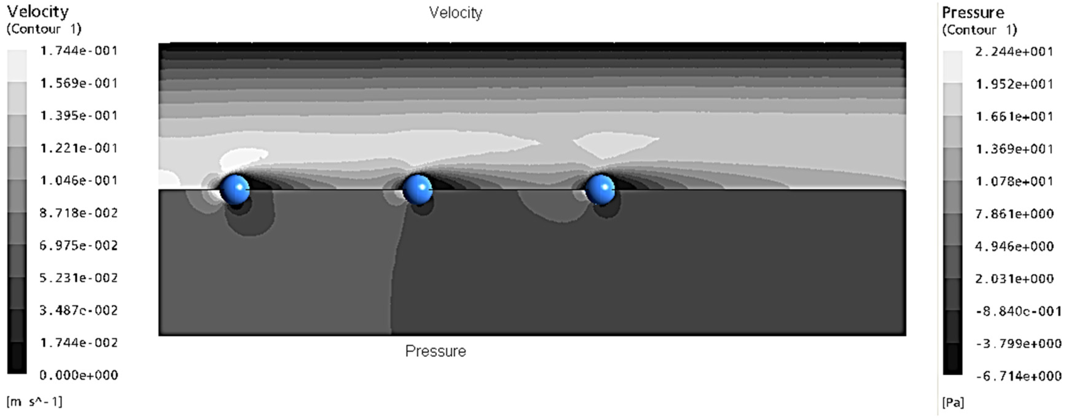
Figure 6 shows the velocity contour plot of the present CFD study at a separation distance of 5 particle diameters and a Reynolds number of 54. The leading particle is subjected to higher velocities than the trailing particles which in turn leads to the higher drag force.
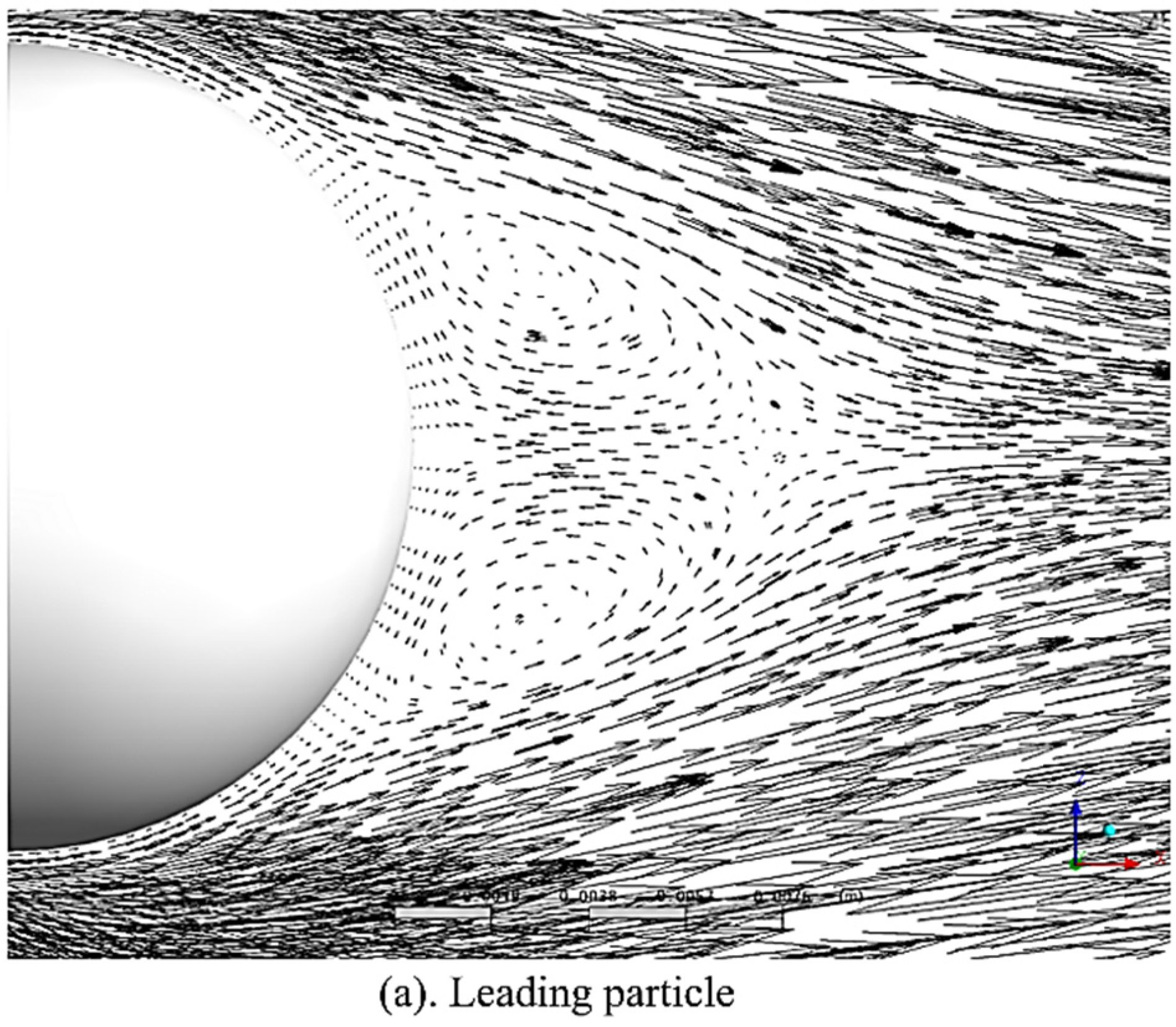
Figure 7 shows a close-up view of the recirculation area behind the three particles. The leading particle, due to the higher incoming velocity, has a larger recirculation area and results in higher drag forces. Due to the close agreement of the predicting ability of the CFD model, it is valid to assume an accurate extension of this work could be undertaken.
To fully help understand the phenomenon at work in the particle drag of clusters of particles, it is necessary to consider various cases. In the present work, three different cases were investigated:
  • Model 1 investigates the drag force of an average particle within an infinite line of particles co aligned with the flow direction. This model will highlight the effects of inline wake characteristics.
  • Model 2 considers a particle surrounded by an infinite plane of particles aligned perpendicular to the flow to investigate the influence of neighbouring particles.
  • Model 3 investigates an infinite matrix of particles, which is a combination and extension of the previous two models.
The results of cases 1 and two are for comparative purposes only and necessary to fully understand the effect of position and location of particles on surrounding particles.

4.1. Particles Aligned with Flow (Model 1)

Model 1 looks at the case of infinite number particles co-aligned with the direction of flow (see, Figure 8a). This Model highlights the influence of particle wake on the drag force when aligned with the flow direction. The ranges of the simulations completed for this Model 1 include particle separation distances of 1 to 20 particle diameters and particle Reynolds numbers varying from 1 to 50.
In order to accurately model an infinite number of particles in flow direction, the inlet and outlet regions (see, Figure 8b), require a periodic boundary condition. The periodic boundary condition forces the quantities leaving the domain to be reintroduced into the domain through the inlet patch. The drag force created by the fluid moving passed the particles results in an energy loss due to friction between the shearing layers of fluid adjacent to the particle surface. The periodic boundary condition forms an endless loop of fluid that unless corrected will eventually stall. To overcome this phenomenon an equal amount of momentum is introduce evenly throughout the domain to ensure continuous flow.
To test the introduction of firstly the momentum introduction method and the periodic boundary condition, a pseudo-isolated particle was simulated (separation distance of 80 pd) at various Reynolds numbers and compared with commonly accepted relation for drag force of isolated particles ( F D = 1 2 C D ρ A V 2 where C D = 24 Re 1 + 0.15 Re 0.687 ). Figure 9 shows the close agreement between the theoretical value based on an isolated particle and the CFD simulations. In the cross-stream direction, the effects of the wall on the flow characteristics needed to be removed so a series of geometries were tested at varying distances to determine the minimum distance from the wall for the simulation. It was found the use of 20 d wall distance removed all wall effects from the flow. At a distance of 20 d, a symmetry boundary or free slip (shear stress = 0) was used. This kind of boundary condition removed the drag due to wall friction as is seen in pipe flows.
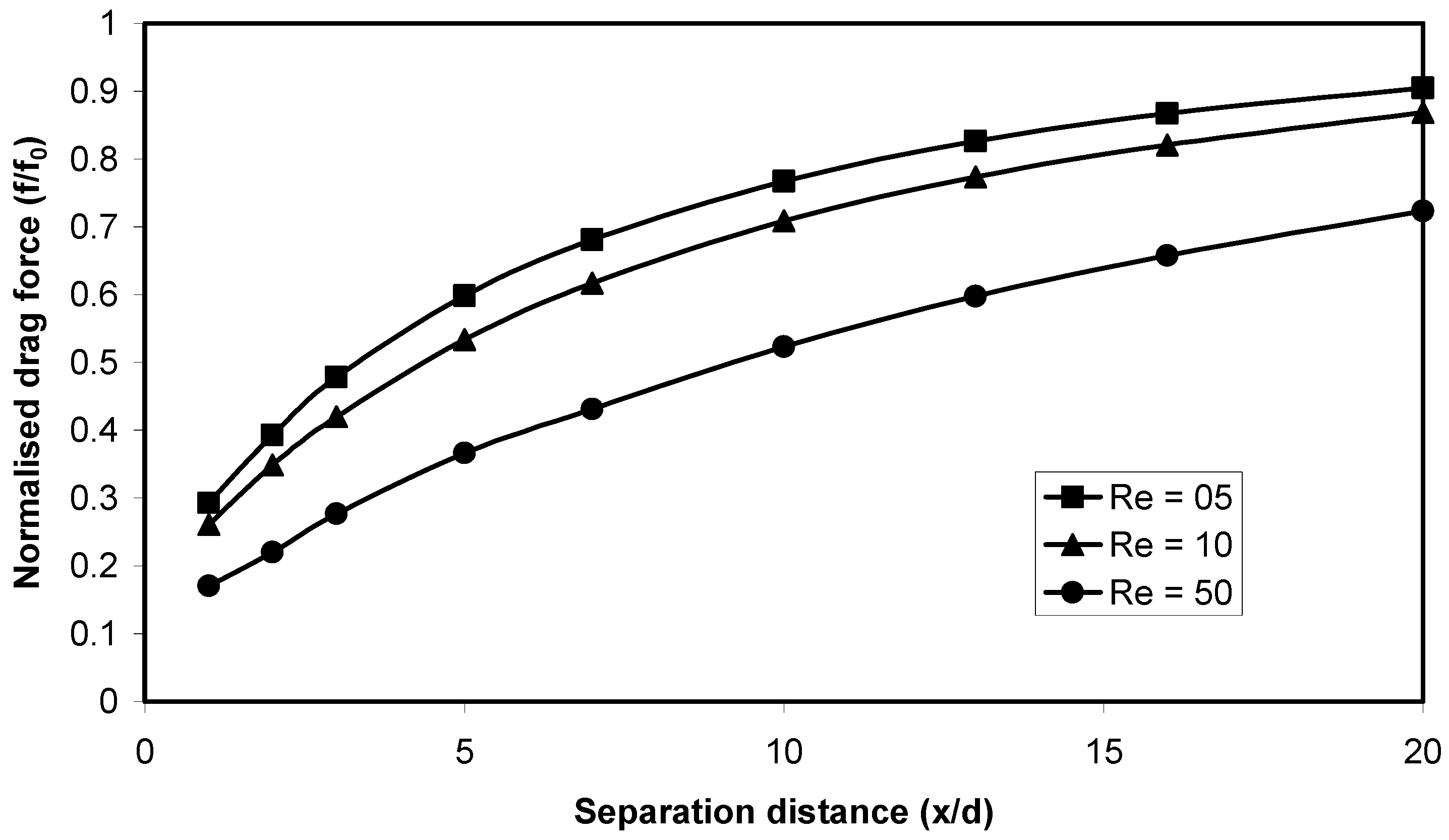
Figure 10 shows the normalised drag force plot for Model 1, where f is the predicted drag force on the test particle and f0 is the corresponding drag force for an isolated particle. It can be noted that at very small separation distances, which represents high particle volume fractions, the reduction of drag is large for all Reynolds numbers. The larger the Reynolds numbers the greater the reduction in drag force. At a separation distance of 1 particle diameter and a Reynolds number of 50, the average particle drag force is approximately 18% of that of an isolated particle at the same Reynolds number. This is the phenomenon that is used by birds to fly great distance by sharing the drag force between the birds. The experimental work of Katz and Meneveau [29] experimentally studied the rise velocity of interactive bubbles and considered the relative between two identical bubble and several separation distances. The results suggest the relative velocity between the particles increased at smaller separation distances. This is consistent with the CFD predictions shown whereby a reduction in drag force would correspond to an increase velocity of the trailing bubble leading to greater relative velocity between to the two bubbles.
The velocity contours for some limited cases of Model 1 are shown in Figure 11. These plots highlight the reason the drag force at smaller separation distances. At 1 particle diameter separation distance, the wake from the previous particle engulfs the trailing particle leading to lower oncoming fluid flow velocity and consequentially lower drag force.

4.2. Particles Perpendicular to Flow (Model 2)

Model 2 investigates the effects of particles located perpendicular to the flow (see, Figure 12a). The range of separation distance for this case includes 1 to 20 particle diameters. Model 2 focussed on the influence of neighbouring particle perpendicular to the flow direction and as such the cross-sectional dimensions were important. The length of the geometry was set to double the separation distance of the particle to the side boundaries. The geometrical design yields little effect on the drag force with the outlet set at this ratio to the side boundaries. This case required an infinite plane of particles perpendicular to the flow to be simulated. This plane is the product of using symmetry boundaries again on the wall regions parallel with the flow, but with this case, the distance to the symmetry boundary will varying accordingly to the separation distance being modelled. (See Figure 12b).
Looking at the drag force results for Model 2 (see, Figure 13), the drag force on the test particle sharply increased compared to that of an isolated particle at the smallest separation distance whereas all the results showed a normalised drag force greater than unity with the greater separation distances showing very little difference from unity. The main reason the increase in drag force is due to the higher velocity experienced by the particle due to the fact that the cross section for the flow to move through decreases past the particle causing the velocity to increase to conserve continuity. This would explain why the results for the smallest geometry are so extreme because this is the case where the flow reduces the most. For example, the case of a separation distance of 1 particle diameter reduces the cross-sectional area past the particle by approximately 20%. Following along the same lines of thinking the smaller Reynolds number results provide greater force increases because the rate of change of drag coefficient and hence drag force with respect to Reynolds number is greater at lower numbers thereby leading to higher experienced drag force as the increase in seen velocity results in higher Reynolds numbers.
The increased drag force attributed to the squeezing of the flow or the ‘nozzle’ effect was also noted by Chen and Lu [30]. In their experimental work, the drag force on 2 and 3 particles positioned side-by-side in the oncoming flow were measured. Their results suggest that at smaller separation distances, the drag force increases, which they primary conclude is based on the nozzle effect, which causes a rise in local Reynolds numbers. Although there is some difference in the magnitude of force increase between the predicted CFD results and those of the experimental work (see, Figure 14), it is noticeable from their work, that the case of three particle yielded slightly higher drag force increase compared with those of the two-particle case. With this in mind, the infinite array of particles perpendicular to flow in these CFD predictions would naturally expect to produce higher drag forces due to introduction of additional particles.
The velocity contour plots of Figure 15 show how the smaller separation distance greatly increases the maximum normalized velocity. The case of separation distance of 10 x/d shows almost a constant normalized velocity of close to unity resulting in a drag force ratio of approximately the same magnitude. This highlights the importance of the “nozzle” effect on the drag force for the smaller geometries caused by close neighbouring particles.

4.3. Infinite Matrix of Particles (Model 3)

The final model consisted of a combination of Models 1 and 2 to form an infinite matrix of particles from which a new drag force was developed (see, Figure 16a). The geometry for Model 3 consisted of a cubic shape of dimensions based on separation distance. As would be expected being a combination of Models 1 and 2, the combination of boundary conditions were also applied to this model. As in Model 1, the periodic boundary condition and introduced momentum were used in Model 3. From Model 2, the symmetry boundary conditions were used (see, Figure 16).
Results for the drag force of Model 3 are seen in Figure 17. For all the cases, there was a sharp increase in drag force at the smaller separation distances similar to that noted for Model 2. This increase again is caused due the increase of perceived velocity seen at the particle due to the constriction in the flow due to the physical presence of the particle. This would also explain why the effect is less noticeable at the greater separation distances. Also of interest is that as the Reynolds number increases the constriction effect is dramatically reduced mainly in part to fact that as rate of change of drag coefficient with respect to Reynolds decreases dramatically at higher Re.
Figure 18 shows the velocity contour plots at various separation distances ranging from 10 to 1 x/d. At the smallest separation distance, it can be easily seen that the wake of the previous particle continues to the next, generally, this result in a reduction of drag force but due to the constriction effect previously discussed, the drag is higher. The constriction effect is highlighted in the contour’s plots, as the normalised velocity of the smaller separation cases is higher than those of the 10 x/d case.
A series of comparison graphs of the three models are shown in Figure 19. The first graph shows that at low Reynolds numbers, the results for Model 3 and Model 2 are almost identical. This is due mainly to the constriction effect discussed early in the chapter. At a Reynolds number of 5 and above it is clear to see distinction between the models. Again, all the results show the sudden increase of drag at smaller separation distances due to the change of flow area, something that is not seen in Model 1 because the wall boundaries were set far enough away to minimise any area change to negligible proportions. For the higher Reynolds number cases it can be seen that apart from the sudden increase at smaller separation distance, as the particles spread, the results replicate the trends seen in Model 1 with the magnitudes of the drag force reduction slightly smaller as it approaches unity.
Figure 20 shows the differences between Model 1 and 3 under the same flow conditions. It can be seen that the wake length produce in Model 1 is greater than that produced by Model 3. The difference in the models is the effect produced by the introduction of neighbouring particles upstream. It is interesting to note that effect of Model 2 beyond 5 particle diameters of separation distance was seen to be negligible, further downstream these particles impact on the wake length shortening and consequential drag force increase. The normalised drag coefficients shown in Figure 21 reinforce the influence of neighbouring particles from Model 2 as there is a clear differential between Model 1 and 3.
The fitment of an equation to predict the drag coefficient of a spherical considering both Reynolds number and particle concentration (α) is based on the results seen in Figure 22. The equation development is based on Reynolds number between 1 and 50 and separation distance of 5 to 20 x/d. The separation distance corresponds particle volume fractions of 10−2 and 5 × 10⁻⁵. To generate an equation for the data obtained from the present CFD prediction in the previous sub sections, a least squares method was utilised. A generic form of the equation was generated as seen in Equation (9). The least squares regression program solved for the constant A, B, C and D.
C D = 24 Re 1 + 0.15 Re 0.687 + A Log π 6 α 3 B + C [ Log ( Re ) ] D
Substituting in the values from Table 2, the generic equation takes the form of Equation (9).
C D = 24 Re 1 + 0.15 Re 0.687 + 0.000353 Log π 6 α 3 15.93 0.16 [ Log ( Re ) ] 3.62
The results were more accurately predicted for those particles whose sizes were closest to the average diameter. Of the three different particle size ranges, the medium particle with an average of 226 μm produced the best CFD predictions with almost perfect predictions. The cases of the larger and smaller particle sizes (342 μm and 136 μm respectively) while still showing improved predictions; they were not as prominent as the medium case. Several limitations to this newly developed drag model need to be acknowledged. Firstly, the particle concentration (α) range for this formula is considered to be adequate for the purpose of modelling dilute flows using the Lagrangian framework. In simulated flows where regions exceed the 0.01 volume fraction, limitations on the newly developed drag force, require the particle drag to be calculated using the standard drag model. This is not considered to be such a problem because at high particle concentrations (α) the particle motion is governed predominately by inter-particle collisions and less by drag force. Secondly, the limitation set on the particle Reynolds number is also considered to be adequate for the use in industrial type flows where the transport of small particles (less than 1 mm) is to be considered whereby generally the local particle Reynolds number would rarely exceed 50. In the case of larger particles producing the particle Reynolds numbers greater than 50 the new drag force will not be used, and the standard drag model would then be used. Finally, the present developed drag force formula has been calculated on a study of the relationship between the drag forces of mono-sized particles. Particles of differing diameter will obviously affect the resulting wake size and consequently the amount of drag reduction seen by trailing particles. A smaller particle (i.e., dp ≥ 136 μm) will not reduce the drag force as significantly on a larger particle (i.e., dp ≤ 342 μm) as would be expected if the situation were reversed. With this in mind, narrow particle size distributions are best suited for use with this formula, as the particles would be considered almost mono-sized. Any particles outside of this narrow band would be subject to incorrect reductions in drag force, particularly smaller particles, which may lead to variations from any validating experimental data. Although this limitation would exclude many applications if the new formula were to be used although the reductions in drag force may not be entirely accurate, it would still yield improvement over the standard drag force model.

5. Summary and Conclusions

The present work accurately reproduced the drag force results seen in the Liang, Hong and Fan [19] experimental study of three co-aligned particle at various separation distances. An extension of this work resulted in the CFD study of three models of varying particle configurations. Model 1 highlighted the important influence that particle wake has on the drag force of trailing particles. From this study, it was found that a trailing particle at small separation distances and a Reynolds number of 50 experience a reduction of up to 80% of drag force. Although not as prominent as this case all scenarios resulted in reduction of the seen drag force with this model. Model 2 considered the effect of neighbouring particle perpendicular to the flow. In all cases, the drag force increased due to a squeezing of the flow at the constriction, as expected this was much more prominent at the smaller separation distance. Most notably at a separation distance of 1 and a Reynolds number also 1 the drag force increased by over 250%. Beyond about 5 particle diameters this effect was almost negligible with drag approximating those of isolated particles at the same Reynolds numbers. For Model 3 for which the new drag equation was developed, at smaller separation distances its behaviour mimics that of Model 2 again because of the squeezing of flow. As the separation distance increased, the results followed more of the results seen for Model1. For both extremes, the increase or reduction of drag force were never as high as the results seen the models whose behaviour it was following. As the application of a new drag force model is to be used primarily for Lagrangian particle tracking where dilute flows are of most interest the range of separation distance was reduced to 5 to 20 particle diameters. This firstly made the fitment of a curve to the data easier and more accurate and secondly the importance of the drag force in dense phase flow becomes secondary to those of particle-particle collisions above and beyond a volume fraction of 0.01, which represents 5 particle diameters of separation distance.

Author Contributions

D.D. and J.N. conceived of the presented idea. D.D. developed the theory and A.A.R.S. performed the computations. D.D. and A.A.R.S. verified the analytical methods. J.N. supervised the findings of this work. All authors have read and agreed to the published version of the manuscript.

Funding

This research received no external funding.

Institutional Review Board Statement

Not applicable.

Informed Consent Statement

Not applicable.

Data Availability Statement

Data available on request from the authors.

Conflicts of Interest

The authors have no conflict of interest to declare that are relevant to the content of this article.

Nomenclature

Asurface area of the particle
ACScross-sectional area perpendicular to the velocity direction
CDcoefficient of drag of the particle
Dpparticle diameter
eRestitution coefficient
Fforce on the particle
FDdrag force
kkinetic energy of the fluid in a particular cell
Ldistance between particle centres
mpparticle mass
npnumber of particles per unit volume
Pcollcollision probability
RepParticle Reynolds number
Sϕ, SPϕsource terms
Sijstrain tensor
uvelocity in the ith
Up,gvelocity of particle and gas respectively
VRelrelative velocity
xdistance in the ith
Greek letters
ρ density of the continuum medium
εvolume fraction
ϕvariable quantity
Γϕdiffusion quantity
μViscosity

References

  1. Yan, F.; Luo, C.S.; Zhu, R.; Wang, Z.Y. Experimental and Numerical Study of a Horizontal-Vertical Gas-Solid Two-Phase System with Self-Excited Oscillatory Flow. Adv. Powder Technol. 2019, 30, 843–853. [Google Scholar] [CrossRef]
  2. Senapati, S.K.; Dash, S.K. Dilute Gas-Particle Flow through Thin and Thick Orifice: A Computational Study through Two Fluid Model. Part. Sci. Technol. 2020, 38, 711–725. [Google Scholar] [CrossRef]
  3. Liu, J.; BaKeDaShi, W.; Li, Z.; Xu, Y.; Ji, W.; Zhang, C.; Cui, G.; Zhang, R. Effect of Flow Velocity on Erosion–Corrosion of 90-Degree Horizontal Elbow. Wear 2017, 376–377, 516–525. [Google Scholar] [CrossRef]
  4. Chinenye-Kanu, N.M.; Hossain, M.; Droubi, M.G.; Islam, S.Z. Numerical Investigation of Two-Phase Flow Induced Local Fluctuations and Interactions of Flow Properties Through Elbow. In Proceedings of the 1st International Conference on Numerical Modelling in Engineering, Ghent, Belgium, 28–29 August 2018; Abdel Wahab, M., Ed.; Springer: Singapore, 2019; pp. 124–141. [Google Scholar]
  5. Ariyaratne, W.K.H.; Ratnayake, C.; Melaaen, M.C. CFD Modeling of Dilute Phase Pneumatic Conveying in a Horizontal Pipe Using Euler–Euler Approach. Part. Sci. Technol. 2018, 37, 1015–1023. [Google Scholar] [CrossRef]
  6. Hu, D.F.; Huang, Z.L.; Sun, J.Y.; Wang, J.D.; Liao, Z.W.; Jiang, B.B.; Yang, J.; Yang, Y.R. Numerical Simulation of Gas-Liquid Flow through a 90° Duct Bend with a Gradual Contraction Pipe. J. Zhejiang Univ.-SCIENCE A 2017, 18, 212–224. [Google Scholar] [CrossRef]
  7. Zhou, H.; Huang, Y.; Yang, Y.; Mo, G.; Li, J.; Cen, K. Experimental Measurements of Gas–Solid Flow and Splitting Mechanisms of a Coal Pipe Splitter with a Perpendicularly Arranged Upstream Elbow. Particuology 2016, 25, 143–150. [Google Scholar] [CrossRef]
  8. Kumar Senapati, S.; Kumar Dash, S. Computation of Pressure Drop and Heat Transfer in Gas-Solid Suspension with Small Sized Particles in a Horizontal Pipe. Part. Sci. Technol. 2020, 38, 985–998. [Google Scholar] [CrossRef]
  9. Zhao, H.; Zhao, Y. CFD–DEM Simulation of Pneumatic Conveying in a Horizontal Channel. Int. J. Multiph. Flow 2019, 118, 64–74. [Google Scholar] [CrossRef]
  10. Jain, R.; Tschisgale, S.; Frohlich, J. A Collision Model for DNS with Ellipsoidal Particles in Viscous Fluid. Int. J. Multiph. Flow 2019, 120, 103087. [Google Scholar] [CrossRef]
  11. Kaushal, D.R.; Thinglas, T.; Tomita, Y.; Kuchii, S.; Tsukamoto, H. CFD Modeling for Pipeline Flow of Fine Particles at High Concentration. Int. J. Multiph. Flow 2012, 43, 85–100. [Google Scholar] [CrossRef]
  12. Tu, J.Y.; Fletcher, C.A.J. Numerical Computation of Turbulent Gas-Solid Particle Flow in a 90° Bend. AIChE J. 1995, 41, 2187–2197. [Google Scholar] [CrossRef]
  13. Jones, W.P.; Launder, B.E. The Prediction of Laminarization with a Two-Equation Model of Turbulence. Int. J. Heat Mass Transf. 1972, 15, 301–314. [Google Scholar] [CrossRef]
  14. Banakermani, M.R.; Naderan, H.; Saffar-Avval, M. An Investigation of Erosion Prediction for 15° to 90° Elbows by Numerical Simulation of Gas-Solid Flow. Powder Technol. 2018, 334, 9–26. [Google Scholar] [CrossRef]
  15. Chen, Y.; Third, J.R.; Muller, C.R. A Drag Force Correlation for Approximately Cubic Particles Constructed from Identical Spheres. Chem. Eng. Sci. 2015, 123, 146–154. [Google Scholar] [CrossRef]
  16. Zhang, J.; Fan, L.S. A semianalytical expression for the drag force of an interactive particle due to wake effect. Ind. Eng. Chem. Res. 2002, 41, 5094–5097. [Google Scholar] [CrossRef]
  17. Shang, Z.; Lou, J.; Li, H. CFD of Dilute Gas–Solid Two-Phase Flow Using Lagrangian Algebraic Slip Mixture Model. Powder Technol. 2014, 266, 120–128. [Google Scholar] [CrossRef]
  18. Miao, Z.; Kuang, S.B.; Zughbi, H.; Yu, A.B. CFD simulation of Dilute-Phase Pneumatic Conveying of Powders. Powder Technol. 2019, 349, 70–83. [Google Scholar] [CrossRef]
  19. Liang, S.C.; Hong, T.; Fan, L.S. Effects of Particle Arrangements on the Drag Force of a Particle in the Intermediate Flow Regime. Int. J. Multiph. Flow 1996, 22, 285–306. [Google Scholar] [CrossRef]
  20. Cheng, H.W.; Papanicolaou, G. Flow Past Periodic Arrays of Spheres at Low Reynolds Number. J. Fluid Mech. 1997, 335, 189–212. [Google Scholar] [CrossRef] [Green Version]
  21. Kim, I.; Elghobashi, S.; Sirignano, W.A. On the Equation for Spherical-Particle Motion: Effect of Reynolds and Acceleration Numbers. J. Fluid Mech. 1998, 367, 221–253. [Google Scholar] [CrossRef]
  22. Zhang, J.; Fan, L.S. On the Rise Velocity of an Interactive Bubble in Liquids. Chem. Eng. J. 2003, 92, 169–176. [Google Scholar] [CrossRef]
  23. Dodds, D.; Naser, J. The Effect of Particle Concentration on the Coefficient of Drag of a Spherical Particle. In Proceedings of the 15th Australian Mechanics Conference, Sydney, Australia, 13–17 December 2004; pp. 13–17. [Google Scholar]
  24. Clift, R.; Grace, J.R.; Weber, M.E. Bubbles, Drops, and Particles; Academic Press: Cambridge, MA, USA, 1978. [Google Scholar]
  25. Shuen, J.S.; Solomon, A.S.P.; Zhang, Q.F.; Faeth, G.M. Structure of Particle-Laden Jets-Measurements and Predictions. Aiaa J. 1985, 23, 396–404. [Google Scholar] [CrossRef]
  26. Sommerfeld, M. Modeling of Particle Wall Collisions in Confined Gas Particle Flows. Int. J. Multiph. Flow 1992, 18, 905–926. [Google Scholar] [CrossRef]
  27. ANSYS, CFX-5, Canonsburg, USA. 2005. Available online: https://www.ansys.com/products/fluids/ansys-cfx (accessed on 10 September 2022).
  28. Sommerfeld, M. Validation of a Stochastic Lagrangian Modelling Approach for Inter-Particle Collisions in Homogeneous Isotropic Turbulence. Int. J. Multiph. Flow 2001, 27, 1829–1858. [Google Scholar] [CrossRef]
  29. Katz, J.; Meneveau, C. Wake-Induced Relative Motion of Bubbles Rising in Line. Int. J. Multiph. Flow 1996, 22, 239–258. [Google Scholar] [CrossRef]
  30. Chen, R.C.; Lu, Y.N. The flow characteristics of an interactive particle at low Reynolds numbers. Int. J. Multiphase Flow 1999, 25, 1645–1655. [Google Scholar] [CrossRef]
Figure 1. Uniform particle distribution.
Fluids 07 00331 g001
Figure 2. The effect of the virtual wall inclination on the post collision properties.
Fluids 07 00331 g002
Figure 3. Present CFD geometry based on the work of Liang (1996) and inlet velocity.
Fluids 07 00331 g003
Figure 4. Mesh configuration for the present CFD geometry.
Fluids 07 00331 g004
Figure 5. Validation of the Liang experiment for three co-aligned particles at Re = 54.
Fluids 07 00331 g005
Figure 6. Velocity and pressure contours plot of Liang experiment at a separation distance of 5 particle diameters and Re = 54.
Fluids 07 00331 g006
Figure 7. Velocity vector plot of (a). leading particle, (b). middle particle, (c). trailing particle at x/d = 5d and Re = 54.
Fluids 07 00331 g007aFluids 07 00331 g007b
Figure 8. (a). Configuration for Model 1, (b). Model 1 boundary conditions.
Fluids 07 00331 g008
Figure 9. Validation of periodic boundary conditions.
Fluids 07 00331 g009
Figure 10. Normalised drag force of Model 1.
Fluids 07 00331 g010
Figure 11. Velocity contour plots for separation distances x/d = 10, 5, 2 and 1 at Re= 50.
Fluids 07 00331 g011
Figure 12. (a). Configuration for Model 2, (b). Model 2 boundary conditions.
Fluids 07 00331 g012
Figure 13. Normalised drag force of Model 2.
Fluids 07 00331 g013
Figure 14. Comparison of CFD simulation results for Model 2 and available experimental data.
Fluids 07 00331 g014
Figure 15. Velocity contour plots of Model 2 for separation distances x/d = 10, 5, 2 and 1 at Re = 50.
Fluids 07 00331 g015
Figure 16. (a). Configuration for Model 3, (b). Model 3 boundary conditions.
Fluids 07 00331 g016
Figure 17. Normalised drag force of Model 3.
Fluids 07 00331 g017
Figure 18. Velocity contour plots for Model 3 at Re = 50 and separation distances x/d = 10, 5, 2 and 1.
Fluids 07 00331 g018
Figure 19. Comparison of the normalised drag force of different models at different Reynolds number.
Fluids 07 00331 g019
Figure 20. Comparison of Models 1 and 3 at separation distance x/d = 16 and Re = 50.
Fluids 07 00331 g020
Figure 21. Comparison of normalised drag coefficients for the three different models at a Re = 5.
Fluids 07 00331 g021
Figure 22. Drag coefficients for various Reynolds number of Model 3.
Fluids 07 00331 g022
Table 1. Fluid properties for Liang (1996) experimental replication work.
ρ (kg/m3)µ (kg/m.s)dp (m)Dpipe (m)u0 (m/s) at Re = 54
12060.0570.0158750.1540.16
Table 2. Calculated constants for generic equation.
ABCDRMS Error
15.940.000353−0.163.620.0439
Publisher’s Note: MDPI stays neutral with regard to jurisdictional claims in published maps and institutional affiliations.

