
Analysis of Carleman Linearization of Lattice Boltzmann


1
Tandon School of Engineering, New York University, Brooklyn, New York, NY 11201, USA
2
Fondazione Istituto Italiano di Tecnologia, Center for Life Nano-Neuroscience at la Sapienza, Viale Regina Elena 291, 00161 Roma, Italy
3
Physics Department, Harvard University, Oxford Street, 17, Cambridge, MA 02138, USA
*
Author to whom correspondence should be addressed.
Fluids 2022, 7(1), 24; https://doi.org/10.3390/fluids7010024
Submission received: 25 November 2021
/
Revised: 23 December 2021
/
Accepted: 30 December 2021
/
Published: 5 January 2022
(This article belongs to the Special Issue Rarefied Gas Dynamics)
Abstract
:We explore the Carleman linearization of the collision term of the lattice Boltzmann formulation, as a first step towards formulating a quantum lattice Boltzmann algorithm. Specifically, we deal with the case of a single, incompressible fluid with the Bhatnagar Gross and Krook equilibrium function. Under this assumption, the error in the velocities is proportional to the square of the Mach number. Then, we showcase the Carleman linearization technique for the system under study. We compute an upper bound to the number of variables as a function of the order of the Carleman linearization. We study both collision and streaming steps of the lattice Boltzmann formulation under Carleman linearization. We analytically show why linearizing the collision step sacrifices the exactness of streaming in lattice Boltzmann, while also contributing to the blow up in the number of Carleman variables in the classical algorithm. The error arising from Carleman linearization has been shown analytically and numerically to improve exponentially with the Carleman linearization order. This bodes well for the development of a corresponding quantum computing algorithm based on the lattice Boltzmann equation.
1. Introduction
Computational Fluid Dynamics (CFD) has accompanied computers as an application since their infancy, starting with von Neumann’s program to simulate the weather on the ENIAC machine around the 1950s. Even earlier, in 1922, Richardson described “human” computers computing the weather by hand, estimating that 64,000 of them, each calculating at a speed of 0.01 Flops/s, would be sufficient to predict the weather in real time [1]. Leaving aside human calculators, electronic ones have made a spectacular trek so far, from the few hundred Flops of ENIAC to the exaflop peak performance of the Sunway Oceanlite supercomputer [2]. This has spanned sixteen orders of magnitude in 70 years, close to a sustained Moore’s law rate, doubling every 1.5 years! Amazingly, CFD has been consistently on the forefront of the journey, and it continues to be to the present day. However, when it comes to quantum computing, CFD is yet to capture the limelight it deserves. In this paper, we present a brief survey of current ongoing research work in this direction and a preparatory technique, known as Carleman linearization, aimed at the development of a quantum computing algorithm for the lattice Boltzmann method for fluid flows.
1.1. Early Attempts for Quantum Simulation of Fluids
The earliest attempts at quantum simulation of fluids have been based on the lattice gas or lattice Boltzmann algorithms. The first quantum lattice Boltzmann scheme dates back to the 1990s [3,4]. Around the turn of the millenium, Yepez demonstrated fluid dynamic simulations on a special-purpose quantum computer based on nuclear magnetic resonance (NMR) [5], using the quantum lattice gas algorithm [6,7]. Leading the trail, Yepez has also investigated Burger’s equation [8,9], and entropic lattice Boltzmann models [10]. The latter has found its use in simulation of quantum fluid dynamics and other quantum systems [6]. We have recently seen a divergence towards citing Navier-Stokes as a future direction for papers discussing solving nonlinear differential equations on quantum computers, away from the early physically-motivated algorithms for fluid simulation, as the quantum lattice gas one mentioned above [5,7,8,9]. However, the attempts to revive the physically-motivated algorithms beyond quantum systems [11], by [12,13,14,15] and others, are promising. The work of [13] stands out as it presents itself as a method not of quantum computation per se, but of quantum simulation. The latter leverages the correspondence between the Dirac and lattice Boltzmann equations. We, thus, find a compelling reason [16] to explore lattice Boltzmann as the basis for quantum simulation of fluids, starting with its linearization, explored classically in this paper.
1.2. Carleman Linearization
Carleman linearization appears to cast linearization of a function through Taylor series expansion into matrix form, suitable for use in defining state estimator of a non-linear system of known dynamics as part of the Koopman operator approach, in what is known as Carleman-Koopman operator. The basic idea of Carleman linearization is to introduce powers of the original variable as a variables in the system. The recurrence through which the new equations in the system is defined leads to an infinite dimensional system. The latter is prone to admitting solutions different than those of the original system [17]. The linearization is achieved at the cost of infinite-dimensions. Upon truncation of the resulting infinite-dimensional upper-triangular matrix [18], the accuracy of the approximation also suffers, deteriorating with time, making the truncated system most suitable for asymptotically stable stationary solutions [19]. The error bound for a Carleman-linearized polynomial ODE reduced to quadratic form has been shown, through a power series approach [18], to depend on the initial condition as well as exponentially on time. They recommend discretizing the solution in time, and evaluating other basis functions. Their work has readily been extended by [20] for a quantum algorithm. Apart from discussing the complexity and error bounds of a quantum Carleman algorithm, [20] presented the results for a classical Carleman linearization of Burger’s equation.
2. Lattice Boltzmann
Between the Navier-Stokes equations which model the flow at a continuum level, and molecular dynamics which treat the microscale, LB stands out, representing the fluid as an ensemble of particles at the mesoscale. It stems from the minimal discretization of the Boltzmann kinetic equation. The lattice Boltzmann formulation is readily extensible for a range of physics, from the quantum to the relativistic, giving the method a versatility about which books could be written [21].
The Boltzmann Equation (1) describes the probability density f of the fluid in the position-momentum space, driven by advection due to continuum particle velocity and collision across space spanned by , and time t. To arrive at the lattice Boltzmann formulation, the probability density f from the Boltzmann equation Equation (1) is discretized into Q density distributions, each describing the fraction of fictitious particles: moving in a given D-dimensional lattice, with restricted to speeds , , defined in the directions of the lattice vectors s.
The discretized lattice Botlzmann equation takes the form
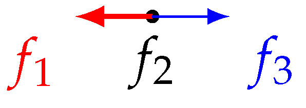
for the simple case of a single-phase fluid, which components are permeable to each other such that they can be considered well-mixed and homogeneous [22]. The discrete probability density is the fundamental variable of the lattice Boltzmann approach. It describes the probability of finding a fictitious fluid particle at a given point defined by the position vector , at a given instant of time t, with a particular speed [23]. Implicit, in the discretization of the Boltzmann equation, is the discretization of the phase-space, involving discrete position and velocity values. The lattice Boltzmann proceeds by updating the discrete probability densities at each cell in two steps: collision and advection/streaming shown in Figure 1. This is the collision step:
The streaming step is:
Collision is practically a relaxation towards equilibrium, a nonlinear operation dependent on terms local to each cell. On the other hand, streaming involves the transfer of the discrete densities to nearby cells, a nonlocal linear operation. The equilibrium distribution is written as a function of the lattice speeds, the fluid density , the lattice vectors , and the flow velocity .
flow velocity :
weights w which sum to unity. A common model for the equilibrium function is:
Replacing the expression for the equilibrium expression for the incompressible case, we have:
We note that the lattice vectors , do not correspond to unit vectors, and are generally not orthonormal. In a single dimension, the left and right vectors have nonzero inner product of . In higher dimensions, we can identify such a pair for each direction, in addition to nonzero inner products with and between diagonal lattice vectors shown in Figure 2. For example, in D1Q3, we have:
thereby:
Continuing with the consideration of the D1Q3 case, by introducing the vectors of first-order and second-order products of the discrete densities appearing in the lattice Boltzmann formulation, denoted and respectively:
we may write as a second-order “polynomial” with matrix-valued coefficients, similar to the form introduced by [18].
where and , for the D1Q3 are:
and:
The constant vector appearing could be absorbed with a fixed variable, say to account for constants. It could easily be defined with a zero derivative adding an empty row to the bottom of and . The constants appearing in any polynomial entry of the vector could be, thus, defined as 1 or multiplied by some coefficient. Therefore, they should not affect the norm of or considered below.
The fact that the rows and columns of sum up to unity, whereas those sum to zero is at heart of the favourable error bounds obtained in Section 3.4, and that in presence of uniform initial conditions or absence of streaming, the method becomes exact. It is well-known that Equation (8) is inconsistent with the incompressible assumption, , and density fluctuations around unity are expected to arise during evolution [24]. Neglecting these fluctuations amounts to an error in the velocity components proportional to the square of the Mach number . This is due to the fact that this standard lattice Boltzmann formulation recovers the compressible Navier-Stokes upon expansion. More sophisticated formulations have been developed for incompressible and nearly incompressible flows [25]. The particles with random motion, are restricted to the lattice nodes with microscopic velocities defined over lattice directions, allowing us to model the collision of particles and their streaming in seperate, uncoupled steps. The latter forces the nonlinearity of fluid flow, captured in the collision term, to be local, whereas the non-local streaming terms remain linear. Moreover, streaming is exact.
Nonlinearity Ratio
We define the nonlinearity ratio R as a measure of how much Equation (8) deviates from a complete linear behavior. It is defined as
where is the matrix of linear coefficients of Equation (8) and is the matrix of the second order terms. Here we have considered the supremum norm of a matrix or a vector as
and as the largest eigenvalue in modulo of . Note that for a linear system such that one has no nonlinearity. This makes R “qualitatively” similar to the Reynolds number which is a ratio of nonlinear convective forces to linear viscous forces. When we rescale a matrix by a constant, its eigenvalues get rescaled as well as the norm. As such, we see that the factor cancels out from the nonlinearity ratio. This is not surprising given that R is practically a measure of the relative weight of nonlinear terms to linear terms. However, this independence of R on a critical parameter, , should be taken with cautiously, as the it role is more nuanced in the lattice Boltzmann formulation.
We may proceed by calculating it for the case of , and it remains valid otherwise.
In the case of D1Q3, the two different norms taken for and both give unity, such that:
where it is less than or equal to 1 by definition of a probability distribution, and where the equality holds in the unlikely case that the distribution is initialized such that a single discrete density is unity. The fact that lattice Boltzmann’s variables are formulated as probability densities is indeed advantageous. While a similar feat could be achieved by rescaling variables for a well-posed problem, as suggested by [20], their relative values and numerical accuracy used limit the effectiveness of such an approach. Moreover, , this means that both conditions set by [20] for arbitrary time-convergence are met. Another advantage of the lattice Boltzmann method is that it is by definition discretized, such that the error arising from discretizing the equation, the forward Euler for time derivative for example as discussed in [20], is irrelevant.
3. Carleman Linearization for Lattice Boltzmann
The basic tenant of Carleman linearization is a change of variables done such that the variables of the original nonlinear system, , are replaced by a larger set of variables . The original variables form a subset of the larger set of Carleman variables. The additional variables are monomials up to order of the original .
Denoting the vector of Carlemann variables of kth order as , and a vector of some polynomial functions of kth order in Carlemann variables, using the numbering scheme shown in Figure 3, we may write:
For lattice Boltzmann with the BGK equilibrium function, we see that the time evolution of each set of monomial of discrete density variables of given order could be written as a function of variables of same order, all preceding orders, and an order above. In Equation (19), we see that those of first order monomials are written in terms of first and second order monomials, and those of second order monomials are written in terms of first, second and third order monomials.
Carleman embedding involves, then, choosing an order of linearization and neglecting higher-order terms from the driving functions of ODEs. This is what we refer to as truncation, and it is demonstrated in Equation (20) to second order, where third-order terms otherwise required for the time evolution of second order terms are dropped.
The Carlemann variables are then introduced to replace the remaining monomials, as shown in Equation (21).
An example of additional variables of second order is shown in Table 1 for a D1Q3 lattice, taking into account the model in Equation (8).
The dynamics of the extended system are then derived from the original system of a single phase, homogeneous, fluid, with terms beyond a chosen order dropped.
which is linearized into the total derivative of the Carleman variables vector equating a constant coefficient matrix, the Carleman linearization matrix C, multiplying the Carleman variables vector:
where the Carleman linearization matrix C is obtained by deriving the following system of equations:
and identifying the variables on the right hand side of Equation (24).
3.1. Number of Variables
An upper bound for the number of Carleman variables for a desired order , when considering N original lattice variables, is
This is an upper bound to the number of Carleman variables used in the linearized system because in practice some terms of order do not appear in the linearized equations. For example, from Table 1 , the second order term for the rest particles density, does not appear in the D1Q3 formulation. In general, the exact number of variables is given after specifying a lattice structure and an equilibrium function.
3.2. Carleman Linearization of Collision Step
The collision operator Equation (3) can be expressed as a function of the Carleman variables, s. To do that, we go back to Equation (1), and consider collision sans streaming. The total derivative of the discrete densities is described by the nonlinear collision operator on the right-hand side.
This assumes that the obtained solution for the discrete density distribution at each site is streamed exactly, and the nonlinear terms recalculated to evolve the system. While this allows us to isolate the error from the linearization of the collision step, it is undesirable in practice. On another note, the linearization of the collision step allows one to explore other discretization scheme to arrive at the LB formulation from the Boltzmann equation Equation (1). In particular, we conjecture that an implicit scheme for the time discretization would improve the error bounds at the cost of the sparsity of the resulting matrix.
3.3. Carleman Linearization of Streaming Step
Instead, we need to consider Equation (1). Another limitation of considering only a traditional one-dimensional model, such as Burger’s is that the problem of streaming the coupled terms of the Carleman linearization is avoided [20]. The forward and backward directions of the velocity are accounted for in one velocity variable with its negative and positive values, and derivatives of the velocity are discretized in terms of that one variable as well.
We have thus far considered linearization of the collision step solely. However, for a self-contained quantum fluid simulation algorithm, Carleman streaming must be considered, which leads us to a modified Boltzmann equation for the Carleman variables:
If the partial derivatives are left undiscretized, we have to include additional variables to account for the new terms appearing, contributing to the blowup of variables, and subjecting a description of streaming to truncation. On the other hand, following the same discretization scheme typical of LB, in similarity to the derivation of Equation (2), we arrive at the a modified LB equation where the coefficients of the partial derivatives of the original variables now show dependence on the variables themselves after replacing the expressions of the Carleman variables and computing their partial derivatives. Equation (27) shows an example:
For D1Q3 second order linearization, with , we have :
where we see new terms unaccounted for in the Carleman variables appear combining both nonlocality, and nonlinearity.
Another way to explain the above is that the discrete densities of the particles are weighted by their contribution to the Carleman variables, the new variables of the system , when streamed. When discretizing the equation describing the evolution of the Carleman variables, a coupling between terms at different locations appears due to the different partial derivatives appearing in the term. Therefore, classical Carleman linearization of the lattice Boltzmann formulation exchanges the local nonlinearity of the collision step, with nonlocal linearity of the streaming step to which the linearized collision term is coupled. We note that additional V variables must introduced for the nonlocal coupled terms, i.e., to keep the system linear. This is indeed used for the Burger’s equation in previous literature [20]. However, this further exacerbates the blowup in variable count for the classical Carleman scheme.
This leads to the fact that streaming is also described by an infinite differential system that must also be truncated. That is, the exactness of streaming, a major advantage of the lattice Boltzmann method, is lost. On a classical computer, to study the collision step, it is possible to recalculate the nonlinear terms to achieve exact streaming. Remarkably, while Carleman linearization slashes out the exact streaming advantage of lattice Boltzmann, we are able to retrieve it by going into the quantum paradigm Itani et al. [26].
3.4. Error Bound
In Equation (8), we see that LB fits into a generalized quadratic ODE considered by [18,20], and it is a multi-population extension of the logistic equation suggested by [20] for treatment.
For a given system of differential equations in terms of a set of variables represented by a vector , of which LB is an example, we denote the solution of the exact system as , and that of the Carleman linearized system as . We use the same definition of the error from [18,20], in terms of the max supremum over time of the vector difference of exact and approximate solution normalized by their respective supremum norms:
As we integrate the system of equations, we define the maximum error made as
When using Carleman linearization and the Euler time discretization as in Equation (2), they require [20] the minimum number of Carleman variables N will be a function of as be:
and the largest time-step :
given that all the eigenvalues of are negative real, and .
The above formulas are derived for a single variable quadratic ODE system, , for which and . Furthermore, in [20], it is shown that the dependence of N and with the error is of the form Equations (31) and (32) even when for the Burgers equation. Note that for the LB problem the bounds of Equations (2), (31) and (32) are not valid as the quadratic system is always multivariate--and for typical choices of the equilibrium function, as for a single-phase fluid in Equation (8).
Now we prove that the leading order in the error improves exponentially with the Carleman order, for 1,2 and 3D systems.
Let denote a Carleman variable of rth order, , such that describes the matrix coefficient describing the contribution of to . We have:
and:
such that when streaming is considered:
For the collision-only setup considered for the classically linearized collision term, = 0, such that one is able to verify:
for D1Q3, D2Q9 and D3Q27, “full” lattices, for which the expressions become linear in Carleman variables up to second order. Equation (35) then reduces to:
Dropping the E term, and with further replacements similar to above, one can see that the first order terms depend only on the initial conditions of the second order terms in the whole domain, not only neighbouring cells, and no third order terms are needed. This is to say that turning off streaming resolves the nonlinearity of the problem, as expected.
With streaming, a simple Taylor expansion of Equation (35) shows that Carleman linearization of order yields a solution with error of the order:
If we initialize the flow to be uniform, the inclusion of streaming does not introduce errors as above, as Equation (37) still holds for the initial conditions at the cells are identical, and so is the collision step, such that . At the boundaries, this still holds if they were periodic, but the latter amounts to the trivial case where the kinetic energy of the flow relaxes to zero. The argument for identical evolution for a uniform initial field under periodic boundaries is visualized in Figure 4. Periodic boundaries refer to a fully periodic domain, in all its dimensions, i.e., triply periodic in , which is typically useful for fundamental studies of homogeneous turbulence.
If (one of) boundaries are not periodic, the error is first generated in the collision step at the boundary, and propagated to the interior of the domain. As illustrated in Figure 5, with each time cycle, the error grows, and it propagates further inside, such that we may speak of a numerical error boundary layer. For example, in a pipe with periodic flow, where the error is first generated at the walls of the pipe, rather than the periodic inlet and outlet.
4. Numerical Results
4.1. Logistic Equation
To demonstrate the utility of Carleman linearization, we consider the logistic equation, as suggested by [20].
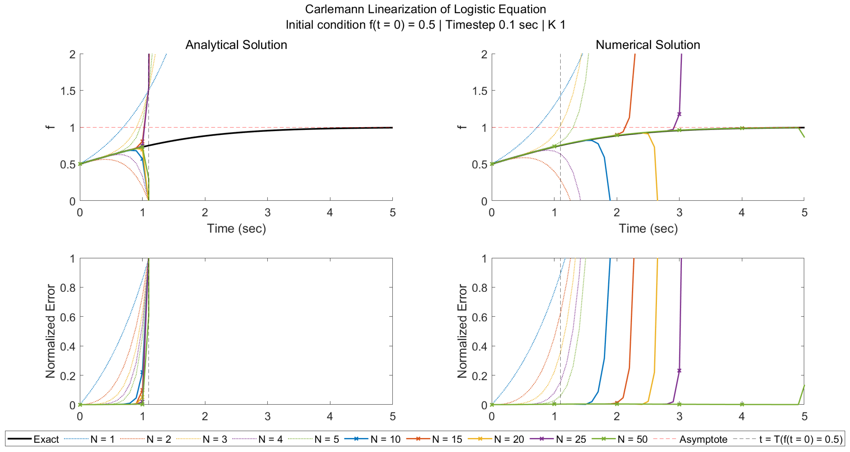
We note that the K factor appears for both first and second order terms, and, thus, cancels out in the calculation of R which remains dependent on the initial conditions solely. In the results, we take . We still see an abrupt cut-off in the utility of the linearization for the resulting analytical solution. This is explained by the fact that even though , the coefficient of the first-order term is definite positive, unity, thereby fulfilling neither [20] nor [18], the conditions set to gurantee error convergence. According to [18,20], this explains the blow-up in the error shown in the analytical solution. Namely, we restate upper-bounds for time T using the power-series method of [18]:
which predicts the time of validity for the linearization as shown in Table 2, and with which the results agree, as the analytical solutions presented in Figure 6.
However, for the numerical solution computed through time-discretization of the equation, we note the error shows slower evolution, giving a longer effective time-period to work with, as could be seen with the numerical solutions extending well-beyond their analytical counterparts before blowing up in Figure 6. Namely, we note that such that their ratio is independent of K, but when the equation is discretized becomes dependent on and the original driving function scaled by , . Thus, the choice of K and weigh on the contribution of nonlinear terms in the discretized equation, such that we expect more accurate solutions for smaller and/or K. This is in line with the findings for the validity of the linearization of the Burger’s equation with , and an invitation for more applied, rather than analytical, work in the field. In terms of lattice Boltzmann, which is defined as a discretized problem, this reveals a shortcoming of using the analytical bounds presented for a general quadratic equation. However, given that Carlemann linearization is exact for a collision-only scheme, and the exacerbation of the blowup of variables when streaming is considerd, as discussed in Section 3.3, this is not investigated on a classical computer, and the results presented for a D1Q3 lattice are limited to a collision-only scheme.
4.2. D1Q3
We now concern ourselves with the results of linearizing the collision term of a D1Q3 lattice Boltzmann formulation. As mentioned in methodology section, exact streaming of the linearized system is only possible on a classical computer with the explicit computation of the nonlinear terms, which defies the purpose of a linearization scheme. Therefore, we restrict ourselves to the collision step only. The test case involves two steps, the first is initializing the discrete densities of a single cell, and the second is performing successive collisions.
where plays a role since we have the contribution of the identity matrix arising from the discretization which does not scale by whereas , as well as and do for that matter.
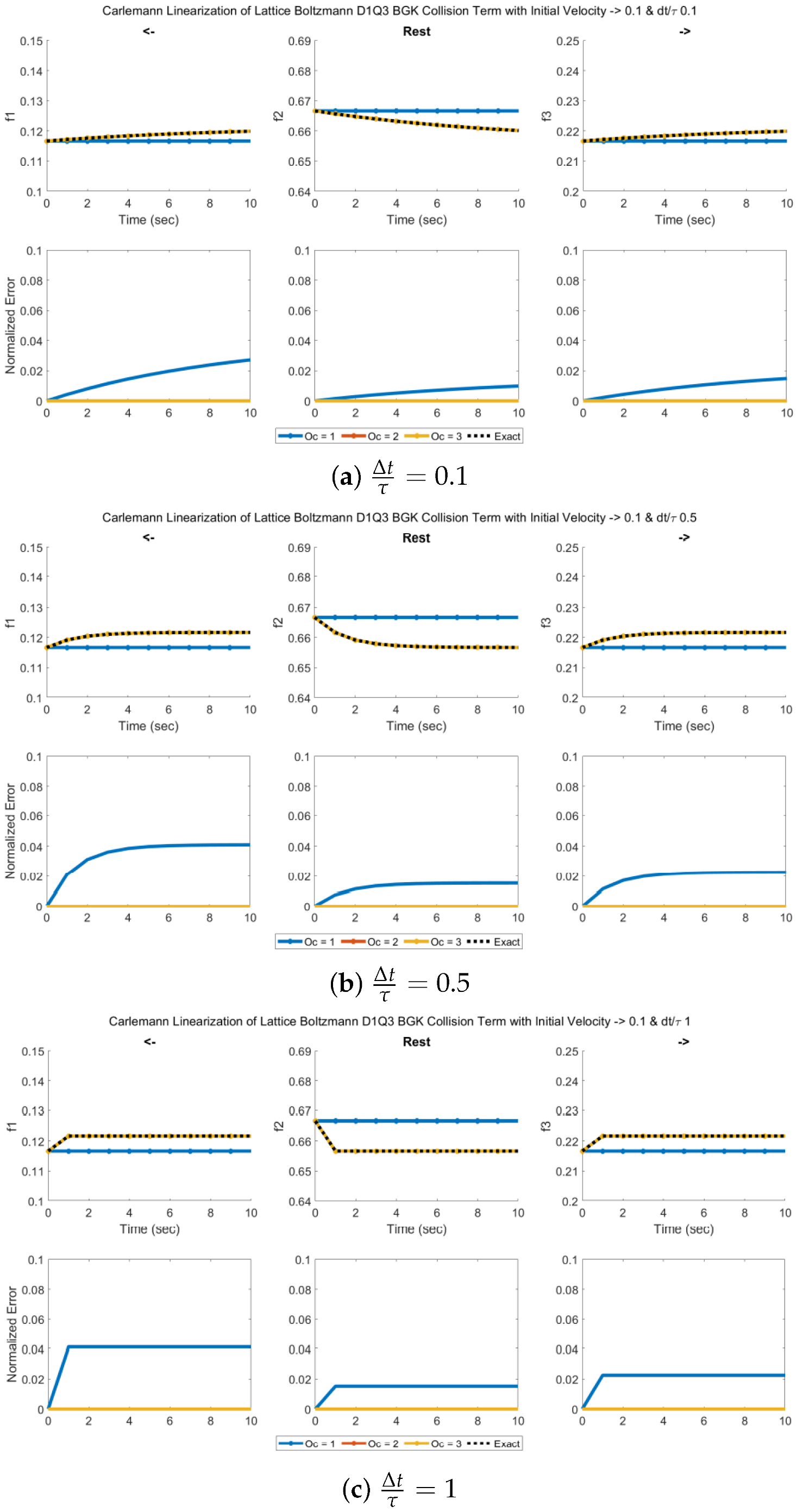
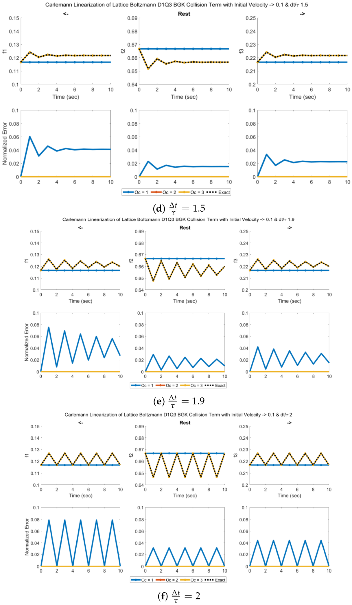
The discrete densities are initialized to differ from the weights of the model by the velocity, chosen to be . In the results shown in Figure 7, the difference has been distributed amongst the left and right discrete densities, such that their difference is u, . We note that this symmetric initialization yields the constant first-order solution shown in blue, but it is not necessary, choosing , for example, has also yielded exact solution from second order during our runs. Apart from the initial velocity, we also experiment with different timestep-relaxation time ratios, varying them between and 2, and we see that the exactness holds. The choice of 2 as a maximum ratio is due to the limitations of the lattice Boltzmann scheme under considerations, as would be discussed below. In the absence of streaming, we see in Figure 7 that the solution is exact for all orders of linearization starting from the second.
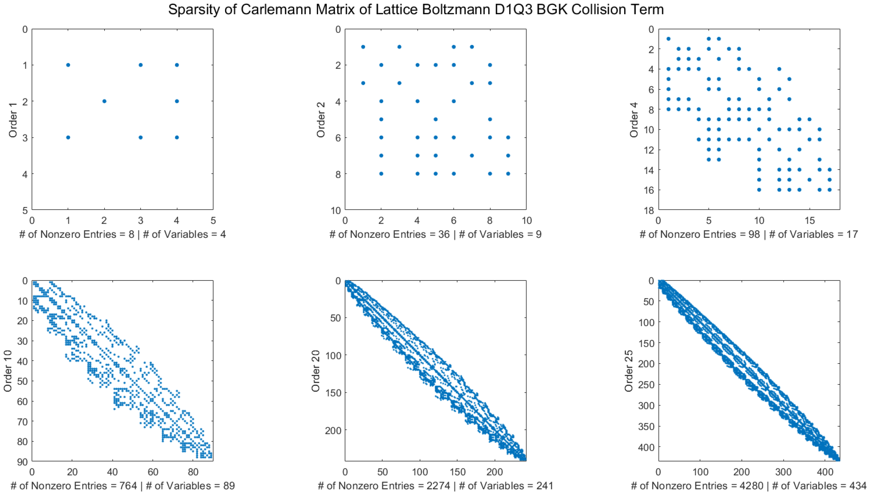
In terms of computing the Carleman linearization matrices, a different approach is used for the lattice Boltzmann scheme than for the logistic equation. In the presence of a single variable, we know apriori the variables that would appear in the linearization, and their derivatives are easily defined either recursively, in relation to one another, or explictly. However, in the case of the lattice Boltzmann formulation, we have found it more efficient to symbolically express the derivatives of each order, starting with the first, identify the variables that do appear in the expression, and then compute the derivatives of the new ones amongst them. As such, we avoid calculating the derivatives of all monomials, some of which never appear in the formulations, such that we have been able to compute the linearization up to 25th order within a handful of minutes on a regular Intel i7-8750H laptop. Apart from the details of the implementation, setting up the Carlemann linearization matrices allows for parallel in time computation, such that one is able to exploit algorithms to calculate powers of matrices, to precompute the matrix for each timestep, irrespective of the initial data.
Moreover, as could be inferred from Figure 8, with increasing linearization order, the Carleman matrix increases in sparsity and approaches a diagonal matrix, becoming more desirable in terms of numerical stability, and even quantum matrix-inversion algorithms.
Dynamic similarity holds for the lattice Boltzmann model of flow under consideration, such that the Reynold’s number is equal in lattice and physical units. In lattice units, we may write it as:
For the single cell considered, without streaming, there is no characteristic length scale. We may instead define it using the characteristic velocity U and the relaxation constant time . The problem setup is that of a flow of decaying velocity, such that we may use the initial velocity u as the characteristic velocity U. Moreover, the kinematic viscosity is defined in lattice units as:
It becomes immediately obvious that is a limitation of the model, or in lattice units, . Even in the vicinity of 2, the model is considered unstable. However, we note that the Carleman linearized system still tracks the original system exactly beyond the range of stability of the lattice Boltzmann model. If we define the Reynolds number for the grid [27]:
and consider the low-Mach number requirement for the incompressibility assumption, typically , we may arrive at the fact that the grid Reynolds number should be of order , which in fact, for a given , is another way of saying that should be chosen in physical units as small enough to capture the long-range structure that arises [27]. As for , the recommendation is that it is slightly larger than unity. Put together, they indicate that the lattice Boltzmann scheme under consideration is fit for . We take the chance here to reiterate the findings that Carleman linearization still exactly tracks the unstable lattice Boltzmann system. Therefore, the limitations on Reynolds number arise from the inherent limitations of the lattice Boltzmann scheme considered. While we expect our findings to extend to other lattice Boltzmann models, this is conditional upon the equations of the extended models and the resulting structure of the coefficient matrices. This paper should be taken as a motivation to investigate other flavours of the lattice Boltzmann method beyond the vanilla flavour considered here.
In terms of Carleman linearization, a larger than unity in lattice units spells good news for the method. It means that the nonlinearity ratio remains bounded by unity even when considering the time discretization:
5. Conclusions
The classical algorithm suffers from a blowup in variable count and sacrifices the exactness of streaming. However, we have shown that the error of the classical Carleman technique could be mitigated, even effaced, in specific applications. On the bright side, we have shown that, at least for the case explored in this paper, the error of the Carleman linearization decreases exponentially with the order of the linearization. This bodes well for the development of a quantum LB algorithm based on Carleman linearization [26].
Author Contributions
Conceptualization, S.S. and W.I.; Methodology, S.S. and W.I.; Software, W.I.; Formal Analysis, S.S. and W.I.; Investigation, S.S. and W.I.; Writing—Original Draft Preparation, S.S. and W.I.; Writing—Review & Editing, S.S. and W.I.; Visualization, W.I.; Supervision, S.S.; Project Administration, S.S.; Funding Acquisition, S.S. All authors have read and agreed to the published version of the manuscript.
Funding
Sauro Succi acknowledges funding from the European Research Council under the European Union’s Horizon 2020 Framework Programme (No. FP/2014-2020) ERC Grant Agreement No.739964 (COPMAT). Wael Itani acknowledges funding from New York University Tandon School of Engineering under the School of Engineering Fellowship 2021.
Data Availability Statement
The MATLAB codes developed for this study are openly available in GitHub at https://github.com/waelitani/Carleman-linearization-lattice-boltzmann (accessed on 27 October 2021).
Acknowledgments
The authors would like to acknowledge Antonio Mezzacapo for the long, fruitful discussions without which major findings of this paper would not have been possible.
Conflicts of Interest
The authors declare no conflict of interest.
Nomenclature
| Continuum particle velocity | |
| Discrete velocity in the ith direction | |
| Q | Number of discrete velocities number of modes at each lattice site, indexed by i |
| D | Number of dimensions of the lattice |
| x | Dimensions of the lattice, indexed by d, independent position vector variable |
| N | Number of Carleman variables |
| Number of sites across the dth dimension of the lattice | |
| G | Volume of the lattice in the units obtained by the product of the number of sites in each dimension |
| Discrete density distribution weight | |
| Collision operator defined by | |
| Weight of the ith discrete density | |
| Truncation order in Carleman linearization | |
| R | Ratio providing measure of nonlinearity parametrizing the error bound of the Carleman technique |
| Coefficient vector of zero-order terms in a quadratic ODE | |
| Coefficient matrix of first-order terms in a quadratic ODE | |
| Coefficient matrix of second-order terms in a quadratic ODE | |
| t | Independent time variable |
| Flow velocity | |
| Local fluid density in lattice units | |
| c | Lattice speed |
| C | Carleman linearization matrix |
| Norm of the solution error | |
| Approximated solution of the system | |
| Discrete timestep | |
| V | Vector of Carleman variables |
| Lattice vectors | |
| Mach number | |
| K | Scaling factor of the logistic equation |
| T | Total integration time |
| p | Order of the polynomial describing the driving function |
| a vector of polynomial functions of kth order in Carlemann variables | |
| Reynold’s number | |
| L | Characteristic length scale defined in units of |
| U | Characteristic velocity in lattice units |
| Kinematic viscosity in lattice units | |
| Speed of sound in lattice units |
References
- Nitzberg, B. Weather Forecasting Gets Real, Thanks to High-Performance Computing. 2017. Available online: https://www.altair.com/c2r/ws2017/weather-forecasting-gets-real-thanks-high-performance-computing (accessed on 25 November 2021).
- Moss, S. China May Already Have Two Exascale Supercomputers. 2021. Available online: https://www.datacenterdynamics.com/en/news/china-may-already-have-two-exascale-supercomputers/ (accessed on 25 November 2021).
- Benzi, R.; Succi, S.; Vergassola, M. The lattice Boltzmann equation: Theory and applications. Phys. Rep. 1992, 222, 145–197. [Google Scholar] [CrossRef]
- Succi, S.; Benzi, R. Lattice Boltzmann equation for quantum mechanics. Phys. D Nonlinear Phenom. 1993, 69, 327–332. [Google Scholar] [CrossRef]
- Yepez, J. Quantum Computation of Fluid Dynamics. In Quantum Computing and Quantum Communications; Williams, C.P., Goos, G., Hartmanis, J., van Leeuwen, J., Eds.; Series Title: Lecture Notes in Computer Science; Springer: Berlin/Heidelberg, Germany, 1999; Volume 1509, pp. 34–60. [Google Scholar] [CrossRef]
- Vahala, G.; Yepez, J.; Vahala, L. Quantum Lattice Gas Algorithm for Quantum Turbulence and Vortex Reconnection in the Gross-Pitaevskii Equation. In Proceedings of the 2008 SPIE Quantum Information and Computation VI, Orlando, FL, USA, 23 April 2008; Volume 6976. [Google Scholar] [CrossRef]
- Yepez, J. Lattice-Gas Quantum Computation. Int. J. Mod. Phys. C 1998, 9, 1587–1596. [Google Scholar] [CrossRef] [Green Version]
- Yepez, J. An efficient quantum algorithm for the one-dimensional Burgers equation. arXiv 2002, arXiv:0210092. [Google Scholar]
- Yepez, J. Open quantum system model of the one-dimensional Burgers equation with tunable shear viscosity. Phys. Rev. A 2006, 74, 042322. [Google Scholar] [CrossRef] [Green Version]
- Boghosian, B.M.; Yepez, J.; Coveney, P.V.; Wager, A. Entropic lattice Boltzmann methods. Proc. R. Soc. London Ser. A Math. Phys. Eng. Sci. 2001, 457, 717–766. [Google Scholar] [CrossRef] [Green Version]
- Boghosian, B.M.; Taylor, W. Simulating quantum mechanics on a quantum computer. Phys. D Nonlinear Phenom. 1998, 120, 30–42. [Google Scholar] [CrossRef] [Green Version]
- Steijl, R. Quantum Algorithms for Fluid Simulations. In Advances in Quantum Communication and Information; Bulnes, F.N., Stavrou, V., Morozov, O.V., Bourdine, A., Eds.; IntechOpen: Rijeka, Licko-Senjska, Croatia, 2020. [Google Scholar] [CrossRef] [Green Version]
- Mezzacapo, A.; Sanz, M.; Lamata, L.; Egusquiza, I.L.; Succi, S.; Solano, E. Quantum Simulator for Transport Phenomena in Fluid Flows. Sci. Rep. 2015, 5, 13153. [Google Scholar] [CrossRef] [PubMed] [Green Version]
- Budinski, L. Quantum algorithm for the advection—Diffusion equation simulated with the lattice Boltzmann method. Quantum Inf. Process. 2021, 20, 57. [Google Scholar] [CrossRef]
- Lloyd, S.; De Palma, G.; Gokler, C.; Kiani, B.; Liu, Z.W.; Marvian, M.; Tennie, F.; Palmer, T. Quantum algorithm for nonlinear differential equations. arXiv 2020, arXiv:2011.06571. [Google Scholar]
- Succi, S. Lattice Boltzmann 2038. EPL Europhys. Lett. 2015, 109, 50001. [Google Scholar] [CrossRef]
- Steeb, W.H. Linearization Procedure and Nonlinear Systems of Differential and Difference Equations. In Nonlinear Phenomena in Chemical Dynamics; Vidal, C., Pacault, A., Eds.; Springer Series in Synergetics; Springer: Berlin/Heidelberg, Germany, 1981; p. 275. [Google Scholar] [CrossRef]
- Forets, M.; Pouly, A. Explicit Error Bounds for Carleman Linearization. arXiv 2017, arXiv:1711.02552. [Google Scholar]
- Steeb, W.H. Linearization Procedure and Nonlinear Systems of DitJerential and DitJerence Equations. In Nonlinear Phenomena in Chemical Dynamics: Proceedings of an International Conference, Bordeaux, France, 7–11 September 1981; Vidal, C., Pacault, A., Haken, H., Eds.; Springer Series in Synergetics; Springer: Berlin/Heidelberg, Germany, 1981; Volume 12. [Google Scholar] [CrossRef]
- Liu, J.P.; Kolden, H.O.; Krovi, H.K.; Loureiro, N.F.; Trivisa, K.; Childs, A.M. Efficient quantum algorithm for dissipative nonlinear differential equations. arXiv 2020, arXiv:2011.03185. [Google Scholar] [CrossRef] [PubMed]
- Succi, S. The Lattice Boltzmann Equation: For Complex States of Flowing Matter, 1st ed.; Oxford University Press: Oxford, UK, 2018. [Google Scholar]
- Bill, Y.; Meskas, J. Lattice Boltzmann Method for Fluid Simulations. 1997. Available online: https://www.researchgate.net/publication/265077140_Lattice_Boltzmann_Method_for_Fluid_Simulations/ (accessed on 25 November 2021).
- Randles, A.P.; Kale, V.; Hammond, J.; Gropp, W.; Kaxiras, E. Performance Analysis of the Lattice Boltzmann Model Beyond Navier-Stokes. In Proceedings of the 2013 IEEE 27th International Symposium on Parallel and Distributed Processing, Boston, MA, USA, 20–24 May 2013; IEEE: Cambridge, MA, USA, 2013; pp. 1063–1074. [Google Scholar] [CrossRef] [Green Version]
- He, X.; Luo, L.S. Lattice Boltzmann Model for the Incompressible Navier—Stokes Equation. J. Stat. Phys. 1997, 88, 927–944. [Google Scholar] [CrossRef]
- Lallemand, P.; Luo, L.S.; Krafczyk, M.; Yong, W.A. The lattice Boltzmann method for nearly incompressible flows. J. Comput. Phys. 2021, 431, 109713. [Google Scholar] [CrossRef]
- Itani, W.; Mezzacapo, A.; Succi, S. Quantum Carlemann Algorithm for Lattice Boltzmann Fluid Simulation. 2021; In preparation. [Google Scholar]
- Krüger, T.; Kusumaatmaja, H.; Kuzmin, A.; Shardt, O.; Silva, G.; Viggen, E.M. The Lattice Boltzmann Method: Principles and Practice, 1st ed.; Graduate Texts in Physics; Springer International Publishing: Cham, Switzerland, 2017. [Google Scholar] [CrossRef]
Figure 1.
An illustration of the D1Q3 lattice Boltzmann scheme showing how the collision step is a relaxation of the discrete densities towards their equilibrium values whereas streaming involves assigning their values to neighboring cells in the respective directions.
Figure 1.
An illustration of the D1Q3 lattice Boltzmann scheme showing how the collision step is a relaxation of the discrete densities towards their equilibrium values whereas streaming involves assigning their values to neighboring cells in the respective directions.

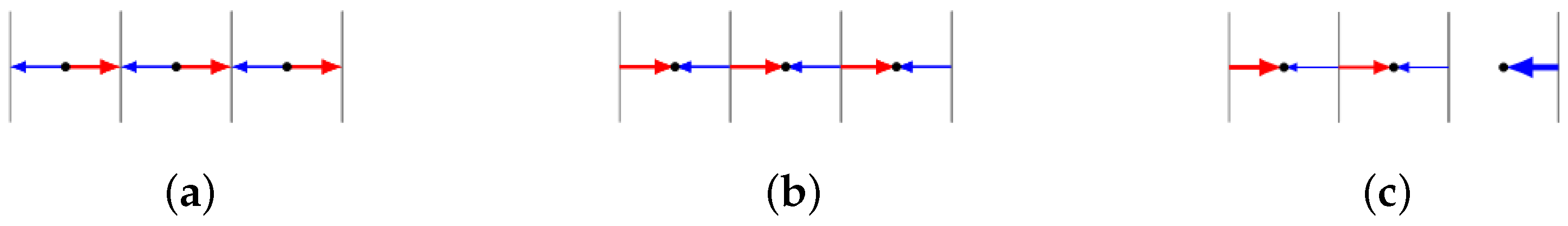
Figure 2.
Different lattice configurations in three (a), two (b) and one (c) dimensions.

Figure 3.
Numbering convention used for the discrete densities of the D1Q3 lattice Boltzmann scheme. In 1D, the lattice vectors correspond to the respective scalars .
Figure 3.
Numbering convention used for the discrete densities of the D1Q3 lattice Boltzmann scheme. In 1D, the lattice vectors correspond to the respective scalars .

Figure 4.
Illustration of how the streaming step preserves uniformity under periodic boundaries only, using D1Q2. The uniform initial flow with periodic boundaries coincides with the error-free case of collision without streaming while errors form at the boundaries when non-periodic boundary conditions are applied. We see that with the same initial conditions and periodic boundary, local and neighboring information of discrete densities are interchangeable. (a) Uniform initial flow field, (b) Periodic boundary conditions, (c) Non-periodic boundary conditions.

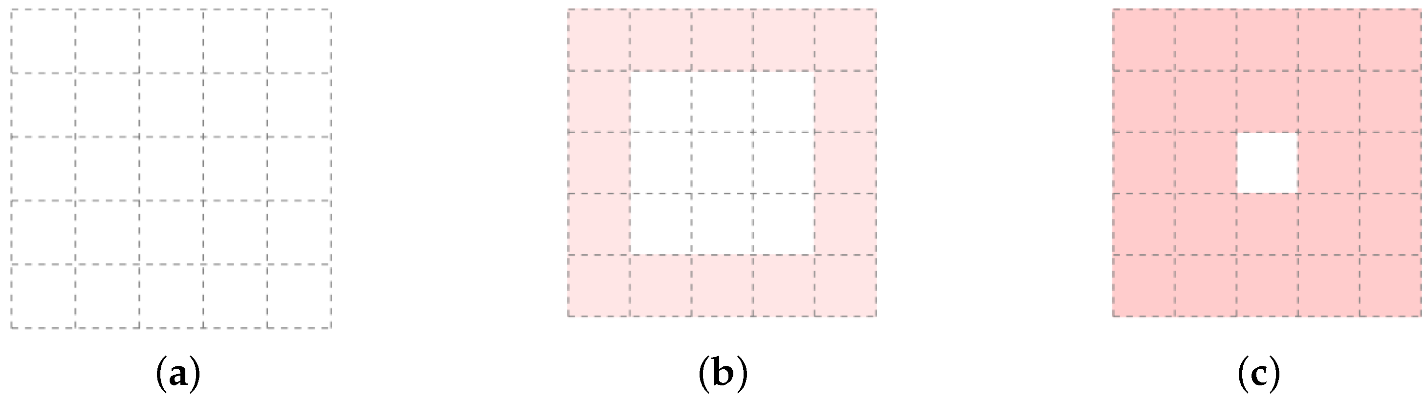
Figure 5.
Illustration of the propagation of Carleman linearization error with timestep in a two-dimensional domain with uniform initial flow and non-periodic boundaries. Lattice cells with no fill have discrete exact discrete densities whereas ones with red fill have discrete densities with error. (a) Initial condition, at , (b) After one timestep, at . (c) After two timesteps, at .

Figure 6.
The analytical (left) (analytical integration) and numerical (right) (discrete time-stepping) solutions of the Carleman-linearized logistic equation are shown with their corresponding errors (bottom) as a function of time, varying initial conditions and Carleman linearization orders. The predicted time of validity is shown as a vertical asymptote in each plot.

Figure 7.
The solution of the discrete densities of the fluid in D1Q3 for successive collisions is shown for different , for the exact and Carleman-linearized formulations as a function of time and Carleman linearization order. The bottom figures show the normalized errors for each discrete density. Note that the solution is exact beyond the first linearization order.


Figure 8.
Visualization of the sparsity of the Carleman matrix for the collision term at various orders.
Figure 8.
Visualization of the sparsity of the Carleman matrix for the collision term at various orders.


Table 1.
Example of D1Q3 expanded to a second order truncation in Carleman linearization, with Carleman variables. Note that the dummy variable is defined to simplify the form of Equation (23).
Table 1.
Example of D1Q3 expanded to a second order truncation in Carleman linearization, with Carleman variables. Note that the dummy variable is defined to simplify the form of Equation (23).
| Carleman Variables | Lattice Variables |
|---|---|
| 1 | |
Table 2.
The maximum endtime validity for Carleman linearization of the logistic equation as predicted by Equation (41).
Table 2.
The maximum endtime validity for Carleman linearization of the logistic equation as predicted by Equation (41).
| T | |
|---|---|
| 0 | ∞ |
| 0.1 | 2.40 |
| 0.2 | 1.79 |
| 0.3 | 1.47 |
| 0.4 | 1.25 |
| 0.5 | 1.10 |
| 0.6 | 0.98 |
| 0.7 | 0.89 |
| 0.8 | 0.81 |
| 0.9 | 0.75 |
| 1 | 0.69 |
Publisher’s Note: MDPI stays neutral with regard to jurisdictional claims in published maps and institutional affiliations. |
© 2022 by the authors. Licensee MDPI, Basel, Switzerland. This article is an open access article distributed under the terms and conditions of the Creative Commons Attribution (CC BY) license (https://creativecommons.org/licenses/by/4.0/).
Share and Cite
MDPI and ACS Style
Itani, W.; Succi, S. Analysis of Carleman Linearization of Lattice Boltzmann. Fluids 2022, 7, 24. https://doi.org/10.3390/fluids7010024
AMA Style
Itani W, Succi S. Analysis of Carleman Linearization of Lattice Boltzmann. Fluids. 2022; 7(1):24. https://doi.org/10.3390/fluids7010024
Chicago/Turabian StyleItani, Wael, and Sauro Succi. 2022. "Analysis of Carleman Linearization of Lattice Boltzmann" Fluids 7, no. 1: 24. https://doi.org/10.3390/fluids7010024