Article

Fluid Flow Characteristics of Healthy and Calcified Aortic Valves Using Three-Dimensional Lagrangian Coherent Structures Analysis

by
Onur Mutlu
1,†,
Huseyin Enes Salman
2,†,
Huseyin Cagatay Yalcin
1,3,* and
Ali Bahadir Olcay
4,*
1
Biomedical Research Center, Qatar University, Doha P.O. Box 2713, Qatar
2
Department of Mechanical Engineering, TOBB University of Economics and Technology, 06560 Ankara, Turkey
3
Department of Biomedical Sciences, College of Health Science-QU Health, Qatar University, Doha P.O. Box 2713, Qatar
4
Department of Mechanical Engineering, Faculty of Engineering, Yeditepe University, Kayisdagi Cad., 34755 Istanbul, Turkey
*
Authors to whom correspondence should be addressed.
Contributed equally to this work.
Fluids 2021, 6(6), 203; https://doi.org/10.3390/fluids6060203
Submission received: 19 April 2021 / Revised: 9 May 2021 / Accepted: 21 May 2021 / Published: 31 May 2021
(This article belongs to the Special Issue Computational Biofluid Mechanics)

Abstract

:
Aortic valve calcification is an important cardiovascular disorder that deteriorates the accurate functioning of the valve leaflets. The increasing stiffness due to the calcification prevents the complete closure of the valve and therefore leads to significant hemodynamic alterations. Computational fluid dynamics (CFD) modeling enables the investigation of the entire flow domain by processing medical images from aortic valve patients. In this study, we computationally modeled and simulated a 3D aortic valve using patient-specific dimensions of the aortic root and aortic sinus. Leaflet stiffness is deteriorated in aortic valve disease due to calcification. In order to investigate the influence of leaflet calcification on flow dynamics, three different leaflet-stiffness values were considered for healthy, mildly calcified, and severely calcified leaflets. Time-dependent CFD results were used for applying the Lagrangian coherent structures (LCS) technique by performing finite-time Lyapunov exponent (FTLE) computations along with Lagrangian particle residence time (PRT) analysis to identify unique vortex structures at the front and backside of the leaflets. Obtained results indicated that the peak flow velocity at the valve orifice increased with the calcification rate. For the healthy aortic valve, a low-pressure field was observed at the leaflet tips. This low-pressure field gradually expanded through the entire aortic sinus as the calcification level increased. FTLE field plots of the healthy and calcified valves showed a variety of differences in terms of flow structures. When the number of fluid particles in the healthy valve model was taken as reference, 1.59 and 1.74 times more particles accumulated in the mildly and severely calcified valves, respectively, indicating that the calcified valves were not sufficiently opened to allow normal mass flow rates.

1. Introduction

Aortic valves are highly dynamic structures in the cardiovascular system that systematically open and close about 3 billion times during the lifetime of a healthy adult [1]. The aortic valve is composed of three half-moon-shaped leaflets, which open during the left ventricle contraction to provide blood supply to the aorta and immediately close to prevent any backflow after the blood ejection. Accurate functioning of these aortic valves is critically essential for the health of the cardiovascular system. Congenital defects and progression of valve diseases prevent the accurate functioning of the leaflets [2]. Leaflet calcification is one of these diseases, in which the leaflet stiffness increases beyond the normal values, and complete valve closure is not observed during the cardiac cycle. The functional deterioration of the aortic leaflets leads to significant hemodynamic alterations, especially around the valvular region. However, clinically monitoring these hemodynamic changes within the entire valve geometry is a challenge for clinicians.
Computational fluid dynamics (CFD) provide an opportunity to numerically model the problem domain and obtain accurate hemodynamic measures for quantifying the complex flow dynamics and associated biomechanical environment developed due to the initiation and progression of the valve disease [3]. In the literature, two-dimensional (2D) [4,5] and three-dimensional (3D) [6,7] geometric models are used for determining the flow dynamics and pressures in the aortic valves. The strong fluid–solid interaction (FSI) between the blood and the leaflets is an integral part of the modeling because the deformations in the solid and fluid domains counter-interactively affect each other [8,9]. In several studies, numerical analyses were performed to determine the optimum prosthetic aortic valve design in case of a valve replacement [10,11,12,13]. Patient-specific aortic valve models were also generated to provide detailed information to clinicians in the decision-making stage, to clarify whether the case necessitated a replacement or not [8,14,15].
In FSI studies, mechanical stresses and wall shear stresses (WSS) on the leaflets are analyzed in order to capture the increase in the stresses depending on the calcific deposits and calcification growth rate [9,16]. In the numerical analysis of the leaflets, flow-induced WSS on the ventricularis surface (i.e., the leaflet surface neighboring to the left ventricle) is observed to be higher compared to the fibrosa surface (i.e., the leaflet surface neighboring to the aorta). This WSS difference between the two sides of the leaflet is considered to be related to the progression of the disease, as the spatially complex low WSS field on the fibrosa side promotes further calcification [17]. In several studies, the hemodynamic changes in the case of bicuspid valve formation were compared to the healthy tricuspid valve flow [18,19,20]. The leaflet asymmetry [21,22,23], strain concentration [3], principal stresses on the leaflets [24], effect of aortic sinus geometry on the hemodynamics [25], and mechanobiological studies [26,27,28,29] are the other fields of numerical investigations for aortic valves.
Most of the computational studies employed the finite element method to solve the governing fluid dynamics equations by utilizing the Eulerian approach. In this approach, specific spatial points in the fluid domain are the main focus of the investigation within the given time points, rather than elucidating the selected flowing particles through the entire domain of interest. The Eulerian approach used in fluid mechanics may be insufficient for an in-depth study of the fluid flow, especially for identifying unique flow regions. On the other hand, the Lagrangian method can characterize many aspects of the fluid flow, such as identifying recirculation regions, vortex structures, stagnation regions, and residence time of fluid particles, by processing CFD analysis results [30,31,32,33,34,35,36,37,38,39,40,41]. This is achieved by tracking the paths of the fluid particles. For example, the use of the Lagrangian coherent structures (LCS) technique can provide differences in the flow structures caused by aortic stenosis. We compared 2D aortic valve models with different Young’s moduli for the leaflets in our previous work, considering healthy and calcified cases using LCS analysis [30]. Once backward and forward finite-time Lyapunov exponent (FTLE) results were obtained from a 2D CFD model, unique vortex structures were determined around the valvular regions for different Young’s moduli [30]. The jet flow area at the aortic valve can be calculated more accurately with LCS analysis based on the patient-specific different stenosis scenarios, and the effectiveness of the existing clinical methods can be improved [31]. In another study, LCS analysis was performed with the data obtained from the experimental model of the heart. Direct flow (DF), delayed ejection fraction (DEF), and retained flow (RF) structures in the heart were determined using backward FTLE and Lagrangian particle residence time (PRT) analysis [32]. These studies showed that LCS is a powerful approach to analyze complex flows such as aortic valve flow accurately. Such assessments are clinically crucial to understand the progression of cardiac diseases under disturbed flows.
In this study, we concentrated on investigating disturbed flow dynamics by elucidating 3D CFD flow domains of healthy, mildly, and severely calcified aortic valve models using LCS analysis. We improved the aortic valve model presented in reference [5] to a 3D state considering the patient-specific parameters determined via B-mode echocardiography images. Highly dynamic valve flow is inherently a 3D phenomenon, and it requires adaptation of 3D geometries for determining the accurate flow structures. In the present study, three different Young’s moduli were defined as the leaflet material to mimic the level of calcification in the valve. Once time-dependent velocity vectors were obtained from the CFD results, FTLE computations, along with Lagrangian PRT analysis, were performed both in forward and backward directions to identify vortex structures and fluid recirculation zones at the front and backside of the leaflets.

2. Materials and Methods
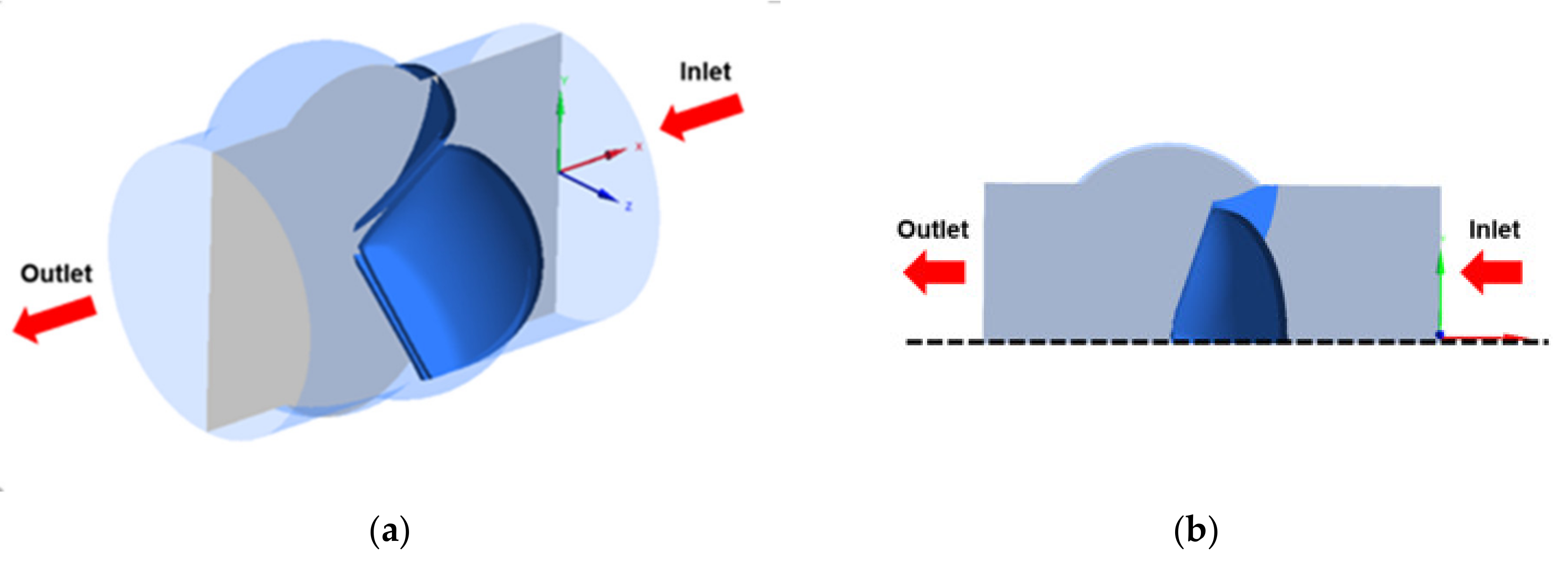
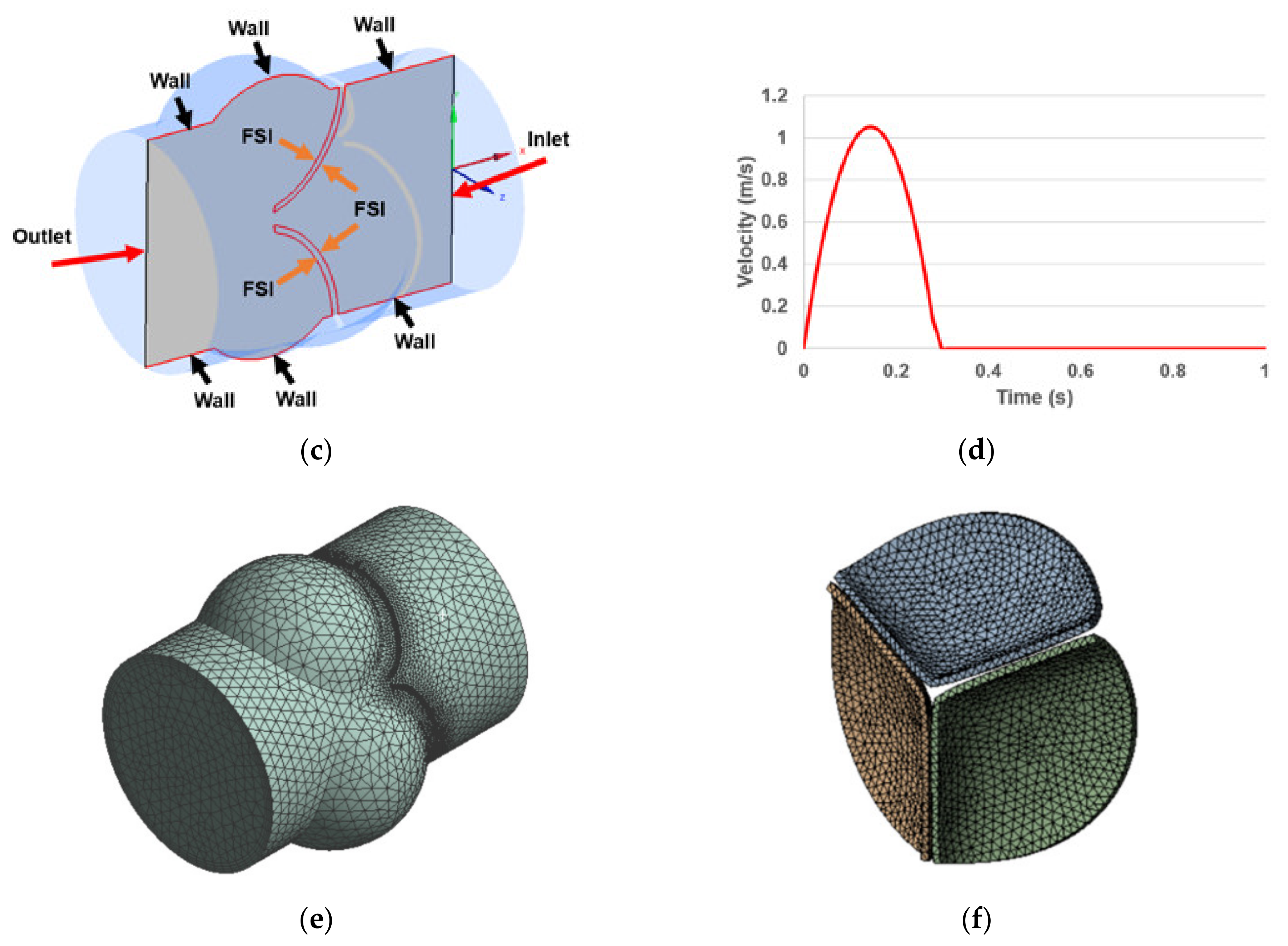
A two-way coupled FSI approach was employed to model the complex dynamic motion of the leaflets and the altered hemodynamics. The fluid and solid domains were modeled separately, and the solutions were coupled at the interaction boundaries using the system-coupling module of ANSYS Workbench 19.2 (Canonsburg, PA, USA). The fluid domain was modeled using ANSYS Fluent to determine the solution field of the flow velocity and pressure. The solid domain was modeled using the ANSYS transient structural module to simulate the leaflet deformations.

2.1. Model Geometry

Parametric dimensions were used as in a previous study [5], and were generated based on the medical images of an adult. Echocardiography imaging (GE Vivid 7 ultrasound machine) was performed to define the dimensions of the geometry using short-axis B-mode images providing the cross-sectional view of the aortic valve. In the model, patient-specific local curvatures of the valve were neglected to obtain a smoothed geometry. The aortic root diameter was measured as 18 mm and modeled with an ideal circular cross-section. Three identical aortic sinuses with spherical configurations were modeled with a diameter of 14 mm and placed at the backside of the leaflet attachment locations. Valve leaflets were modeled with a uniform thickness of 0.4 mm [42]. The aortic valve model employed in the computational analysis is presented in Figure 1.

2.2. Boundary Conditions

The inlet velocity profile of the aortic valve was determined via pulsed Doppler measurements and applied as a plug flow at the inlet boundary [5]. The transient inlet velocity profile is provided in Figure 1d. The outlet of the model was assigned as a zero-pressure boundary. The neighboring surfaces of fluid and solid domains around the leaflets were modeled as FSI boundaries. Aortic root and aortic sinuses were modeled as rigid, and only the leaflets were deformable in the valve model. The surfaces of the aortic root and aortic sinuses were set as wall boundaries. At the FSI and wall boundaries, a no-slip boundary condition was applied, since the fluid particles were stagnant, and there was no flow velocity on these surfaces. In Figure 1c, the boundary conditions are shown on a representative cross-sectional plane. The solutions were obtained for one complete cardiac cycle. A total of 400 time steps were employed with 0.0025 s increments. For the stability of the flow analysis, the CFL (Courant–Friedrichs–Lewy) condition can be checked [43]. The Courant number, which is a measure to define the time step length in the analysis, is recommended to be equal or less than 1 in order to resolve the tiny eddy scales in the domain. The Courant number is defined as U Δ t / Δ h , where U is the magnitude of the flow velocity, Δ t is the incremental time step, and Δ h is the dimension of the mesh element. In our flow analysis, the Courant number reached 10 for the peak flow instant. Since we employed a time-averaged turbulence (k-ε) model, the high value of the Courant number greater than 1 could be compensated for the stability.
It should be noted that assuming zero pressure at the outlet is a primitive modeling approach, and it neglects the flow resistance of the arteries in the body. As a more realistic boundary condition, prescribed pressures changing with time can be assigned at the outlet, and these prescribed pressures can be determined using lumped parameter models [44]. The lack of outlet pressure results in higher peak velocities in the problem domain, leading to increased forces and opening rates on the valve leaflets. Since the valve leaflet opening rates in our computational results were validated with echocardiography images, the zero-pressure outlet condition was used in further computational analyses due to its simplicity.
The solid and fluid domains were composed of 11,435 and 354,614 tetrahedral elements for the generated mesh, respectively. Mesh density was relatively increased around the regions that were close to the FSI and wall boundaries to improve the accuracy of the solution, as presented in Figure 1. Four inflation layers with a growth rate of 1.2 were used for the development of accurate boundary layers on the walls and FSI boundaries. The minimum, maximum, and average skewness of the mesh were 0.000639, 0.892, and 0.226, respectively. The minimum, maximum, and average orthogonal quality of the mesh were 0.107, 0.995, and 0.773, respectively. The convergence issues of the FSI coupling procedures limited the use of a finer mesh, and all computational analyses were performed using the mesh presented in Figure 1. The maximum and average characteristic lengths of the mesh were 0.945 mm and 0.262 mm, respectively, with a standard deviation of 0.175 mm.

2.3. Governing Equations in the Fluid and Solid Domains

The continuity and Navier–Stokes equations were solved for the incompressible flow domain as given in Equations (1) and (2), respectively. In Equation (1), v is the flow velocity vector. In Equation (2), ρ f is the fluid mass density, w is the velocity vector of the fluid domain depending on the FSI based geometric changes, and τ f is the fluid stress tensor.
v = 0
ρ f v t + ρ f v w v τ f = 0
Fluid stress tensor can be defined as given in Equations (3) and (4), where p is the flow pressure, δ ij is the Kronecker delta, μ is the dynamic viscosity of the fluid, and ε ij is the strain rate.
τ f = p δ ij + 2 μ ε ij
ε ij = 1 2 v + v T
The shear strain rate was above 50 s−1 for the large arterial diameters; therefore, the blood could be modeled as a Newtonian fluid with a constant dynamic viscosity of 3.5 cP. For the shear strain rate beyond 50 s−1, the blood behaved as a homogeneous fluid with almost constant viscosity due to the high shear environment [5,45]. The mass density of the blood was used as 1056 kg/m3 [8].
For modeling the turbulent behavior of the flow, a realizable k-ε model was employed, which provided high accuracy in the problems with circulatory flows and flow separation [46]. Realizable k-ε is a Reynolds-averaged Navier–Stokes (RANS) turbulence model based on statistical averaging. The “realizable” term indicates that the model satisfies constraints on the Reynolds stresses in accordance with the physics of turbulent flows. Large eddy simulation (LES) or direct numerical simulation (DNS) approaches can be performed for enhanced accuracy. DNS can resolve even the smallest eddies in the flow. LES computes the largest eddy scales and models the small scales. In order to capture the smallest eddies in the flow, the element dimensions in the mesh should be in the order of Kolmogorov scale ( η ). In Equation (5), the Kolmogorov scale is defined in terms of Reynolds number (Re) and characteristic length (L), which was the aortic root diameter in our problem [43]. The maximum Re reaches 5000 at the peak systolic phase of the flow. According to this peak Re value, the Kolmogorov scale is calculated as 0.03 mm, which requires high computational power. Due to our computational power limitations, we employed a RANS-based realizable k-ε turbulence model. Standard wall functions were used at the proximity of the wall and FSI boundaries to model the physical behavior in the viscous boundary layers accurately. The value of y+ in the flow analysis is recommended to be within the range of 30 to 300 for the proper functioning of the wall functions used in the k-ε turbulence model.
η = Re 3 / 4 L
A transient pressure-based flow solver was employed in ANSYS Fluent due to the incompressible nature of the flow. For the pressure-velocity coupling, the SIMPLEC solution scheme was used with no skewness correction. In this solver, the velocity field was determined from momentum equations, and the pressure field was obtained from a pressure correction equation, which was obtained by using the momentum and continuity equations. The second-order upwind scheme was used for the momentum, and the first-order upwind scheme was used for the turbulent kinetic energy and turbulent dissipation rate. The residual of the continuity equation was used as 10−5 for the solution convergence.
In the solid domain, the momentum conservation is the governing equation, as provided in Equation (6), where τ l is the stress tensor of the leaflets, ρ l is the mass density of the leaflets, and a l is the acceleration vector of the leaflets.
τ l = ρ l a l
A linearly elastic material model was employed in the solid domain with a uniform elastic modulus depending on the level of the valve calcification. For the healthy aortic valve, an elastic modulus of 1 MPa was employed. In the case of mild and severe calcification, the increased leaflet stiffness was modeled using elastic moduli of 10 MPa and 20 MPa, respectively [5]. A constant mass density of 1100 kg/m3 [9] and Poisson’s ratio of 0.45 [23] were employed for the healthy and calcified leaflets.

2.4. FSI Coupling

The dynamic motion of the leaflets is directly influenced by the hemodynamic forces in the fluid domain. Similarly, the deformed state of the leaflets changes the geometry of the fluid domain, indicating a strong coupling between the fluid and solid domains. Therefore, an implicit 2-way FSI coupling approach was adapted to accurately represent the strong interaction between the fluid and solid domains [47,48]. The vector w defined in Equation (2) represents the fluid state vector, and it is obtained by strong (implicit) synchronous coupling. FSI boundaries on the fluid and solid domains were perfectly matched to avoid any misalignment. The fluid domain was remeshed at each new time step to conform to the new deformed state of the leaflet and prevent any convergence problems related to the degenerative cells with negative volumes. For this purpose, spring-based smoothing and remeshing algorithms available in ANSYS Fluent were employed. For the mesh smoothing parameters, the spring constant factor was set as 0.01 with a convergence tolerance of 0.001. For the remeshing parameters, minimum and maximum length scales were set at 0.00127 m and 0.01983 m, with a maximum cell skewness of 0.95. In the case of large structural deformations, new fluid cells were added to the fluid mesh depending on the minimum mesh size criteria. The solution-coupling process between the solid and fluid domains was performed while considering the displacement compatibility and traction equilibrium as provided in Equations (7) and (8), where d l and d f are the solid and fluid displacement vectors, respectively; and n ^ l and n ^ f are the unit normal vectors in the solid and fluid domains, respectively [49].
d l = d f
τ l n ^ l = τ f n ^ f
During the data transfer between the fluid and solid domains, the under-relaxation factor was set at 1 in order to guarantee that the entire force generated due to the blood flow was fully transferred to the solid domain. The root mean square (RMS) convergence target was set as 0.01, and no ramping was applied. Without the use of ramping, the full data transfer value was applied to the target side of the FSI interface during all coupling iterations. At each time step, three FSI iterations were performed for the data transfer.

2.5. Finite-Time Lyapunov Exponent (FTLE) Analysis

The computation of the FTLE field is the most common approach for observing LCS. The FTLE field is a scalar quantity map, which is a measure of the maximum separation ratio between the adjacent particle orbits near each point and is calculated at each point in a computational volume [33]. LCS can be effectively identified when the FTLE fields are calculated by considering the positions of the particles forming the flow relative to each other. LCS can also be seen as equivalent-size structures that maximize FTLE size [50,51,52]. In this study, FTLE fields were calculated by using the velocity results and location information obtained from a plane passing over the centerline of the 3D aortic valve geometry, as seen in Figure 1c. Shadden et al. provided more information on the LCS approach; indeed, the LCS technique was briefly discussed here to illustrate how FTLE fields were obtained for the sake of completeness [51]. The velocity field v(x, t) is obtained by solving the Navier–Stokes equations, in which particle velocity changes with position and time. The positioning of each fluid flow particle as a function of time is thought to be governed by:
x ˙ t ; t 0 , x 0 = v x t ; t 0 , x 0 , t x t 0 ; t 0 , x 0 = x 0
The changing position of the particle at different times gives the particle’s flow map. The flow map is obtained by integrating Equation (9) from time t 0 to time t 0 + τ :
ϕ t 0 t 0 + τ x 0 = x t 0 + τ ; t 0 , x 0
The FTLE is actually a scaling of the right Cauchy–Green strain tensor’s largest eigenvalue. The exponential rate of separation of nearby trajectories, which is a typical characteristic of chaos, is measured by FTLE. FTLE is defined as:
σ x 0 , t 0 , τ = 1 τ t 0 ln λ max C x 0 , t 0 , τ
where λ max C x 0 , t 0 , τ   represents the maximum eigenvalue of the Cauchy–Green strain tensor C x 0 , t 0 , τ . Equation (12) represents the right Cauchy–Green strain tensor, which has a finite-time variant:
S x , t , τ = d ϕ t t + τ x t dx t T d ϕ t t + τ x t dx t
LCS is high-FTLE curves in 2D flows and high-FTLE surfaces in 3D flows [53]. Dispersion in forward time can be seen in the areas surrounding the inflowing manifold. Forward FTLE can be used to receive repelling LCS when τ   > 0. Dispersion in backward time can be seen in the areas surrounding the outflowing manifold. Backward FTLE can be used to receive attracting LCS when τ   < 0.
The particle movements in the computational domain were examined using the PRT method to interpret the LCS analysis results in more detail. Briefly, PRT is a discrete approach used to calculate residence time using particle orbit data. In this approach, massless particles are added into the boundary used in the flow analysis, and these particles are allowed to advance with fluid velocity magnitudes at their locations. PRT measures the amount of time it takes for particles to exit the predefined region and reach the time-varying starting location of the released particle. The positions of these particles are determined using the directions of the velocity vectors obtained by the flow analysis and the time step used in the flow analysis [34].
PRT x 0 , t 0 , Γ = min τ     0 , s . τ . x x 0 , t 0 + τ     Γ
In Equation (13), x 0 is the particle’s initial position, Γ is a region of interest, and the tracer position governs with   x τ = x t 0 + t 0 τ u x s , s   ds .
In this study, 104,291 particles were added to the boundary of the computational volume in every 10 time steps, and the flow of particles was examined. Thus, the PRT method provided information about the formation of the FTLE fields so that the flow hemodynamics resulting from the aortic valve motion could be better understood. In the present study, forward and backward FTLE, as well as the PRT fields, were evaluated for every 0.025 s time-step size and for the total duration of 1 s time length. The solution domain was chosen from −0.0271 to 6 × 10⁻⁵ m in the horizontal and −0.01093 to 0.01133 m in the vertical directions to include both upstream and downstream in the domain. The element size for the computations was selected to be 0.7 × 10⁻⁴; therefore, a resolution of 388 × 318 elements was employed for the analysis.

3. Results

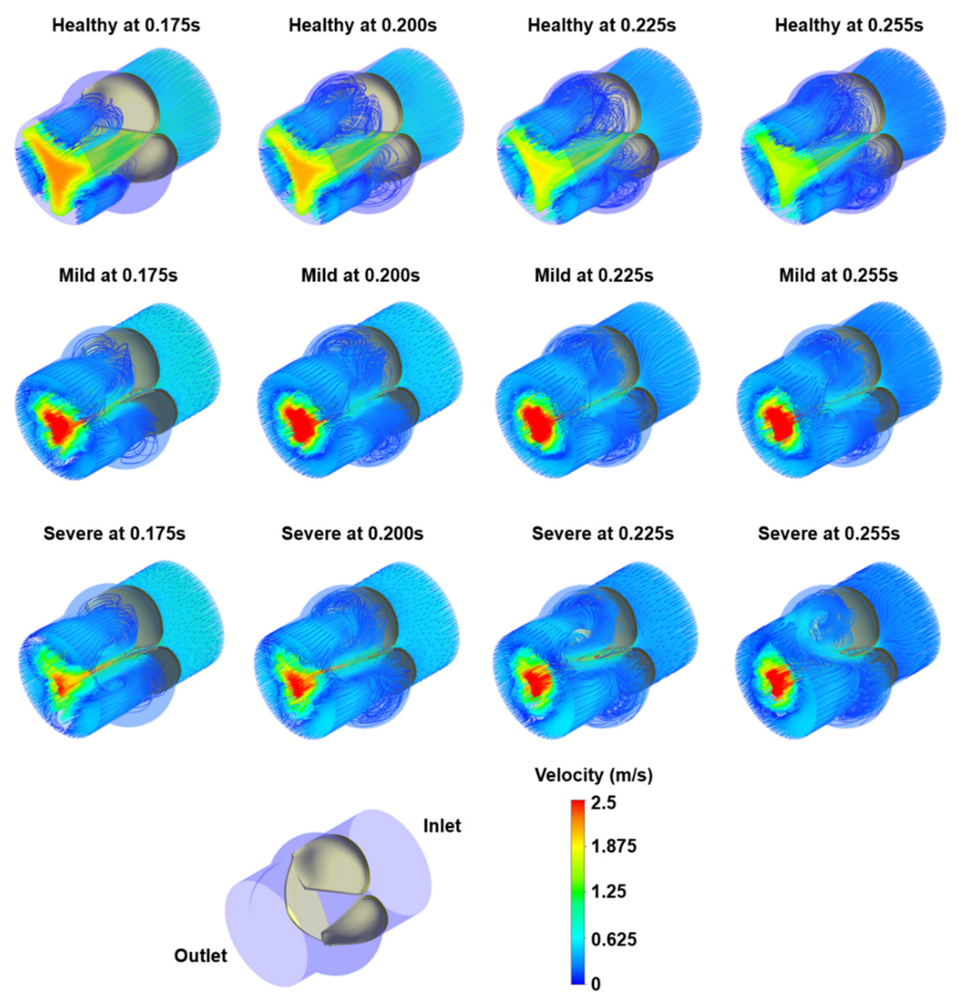
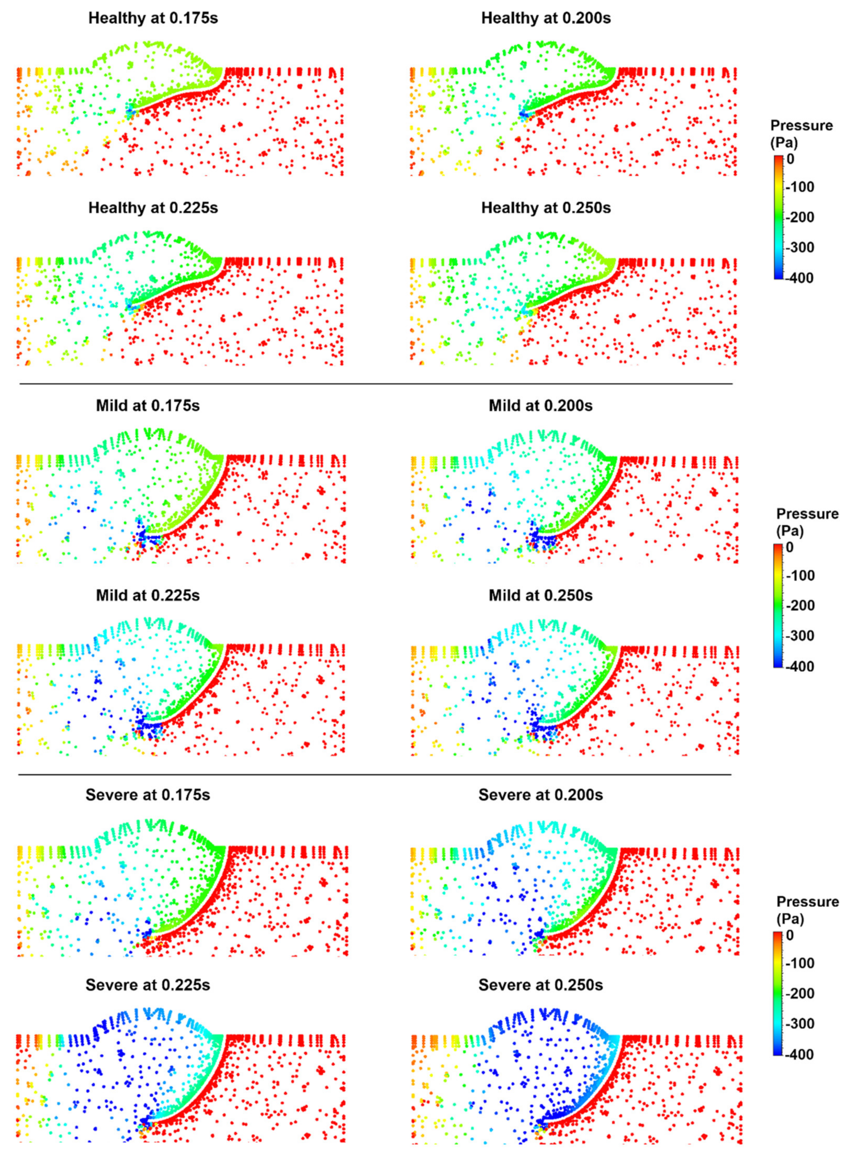
3.1. Flow Streamlines and Pressure Contours

The same inlet velocity profile was applied in all cases; however, peak valve orifice velocities were observed at different time points, indicating a certain time lag. For the healthy valve, peak orifice velocity was obtained as 2.25 m/s at the instant of 0.17 s. Peak orifice velocities were determined as 3.71 m/s and 3.82 m/s at 0.22 s and 0.25 s for the mild and severe calcifications, respectively. The increase in the peak velocity reached 60% in the case of leaflet calcification, consistent with previous findings [5]. 3D flow streamlines are provided in Figure 2 for healthy, mildly calcified, and severely calcified models, demonstrating a laminar flow regime at the upstream of the valve. After passing over the leaflets, flow behavior turned into a turbulent and chaotic form at the downstream. High-velocity jet flow occurred at the valve orifice, and as a result of limited leaflet deformation, the total duration of jet flow increased with increasing calcification. This showed that calcification increased the peak velocity and resulted in circulatory flows in the aortic sinuses. The level of turbulence was directly increased with the increasing calcification rate.
Similar conclusions can also be drawn from the pressure values in the aortic sinuses. The pressure differences with the outlet boundary are presented in Figure 3. The outlet boundary pressure was used as a reference and was set to zero. The pressure differences were plotted on the longitudinal cross-sectional plane for the selected fluid particles. There was a suction region in the aortic sinuses with negative pressure values compared to the outlet boundary pressure. As the calcification level increased, the negative pressure reached about −400 Pa. For the healthy valve, the amplitude of negative pressure was highest only around the tip of the leaflets. In the case of mild calcification, a high negative pressure amplitude spread over a wider region. On the other hand, for a severely calcified aortic valve, high negative pressure dominated almost the entire aortic sinus, with a value of around −400 Pa. These results indicated that the flow hemodynamics were significantly altered in the case of aortic valve calcification.

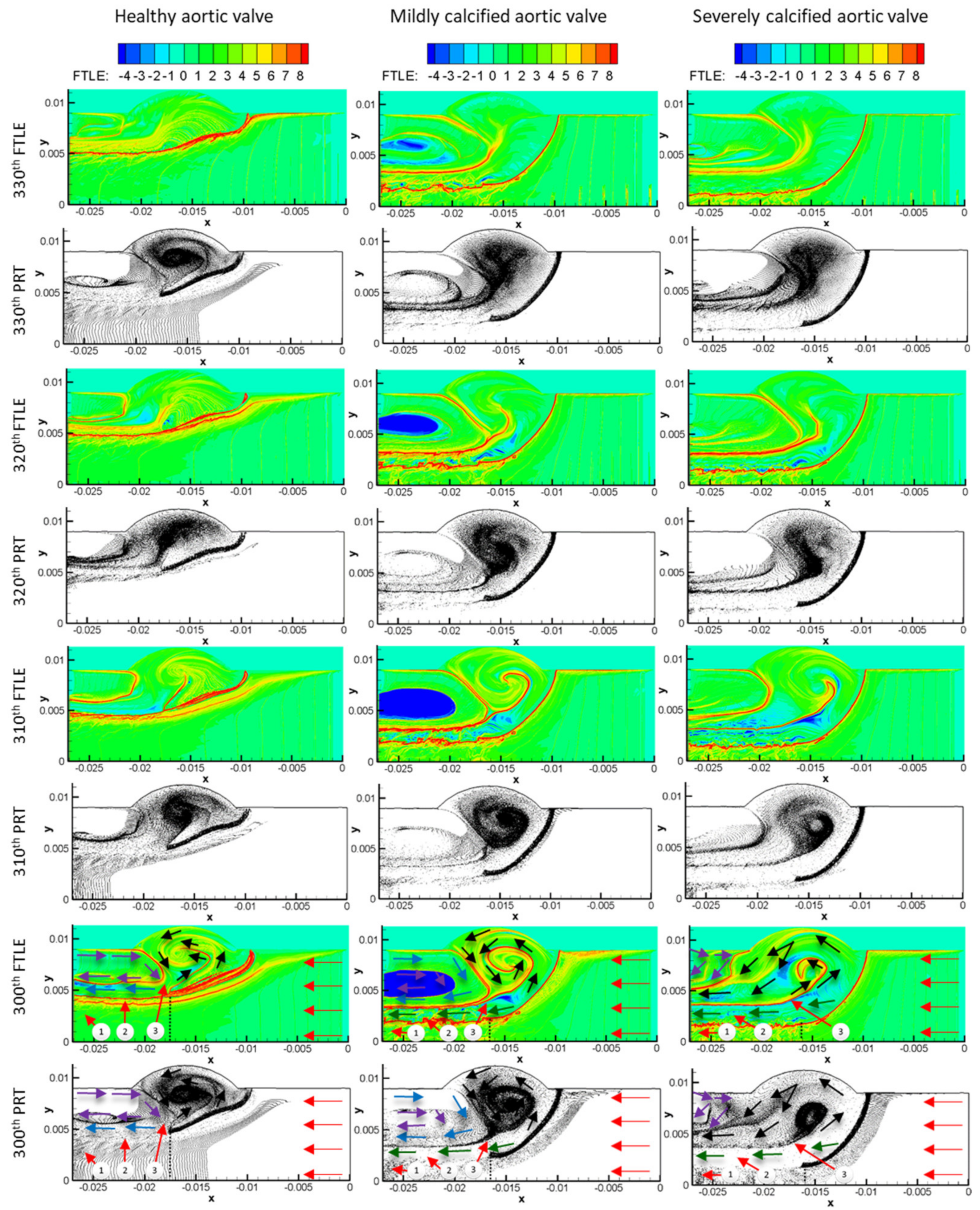
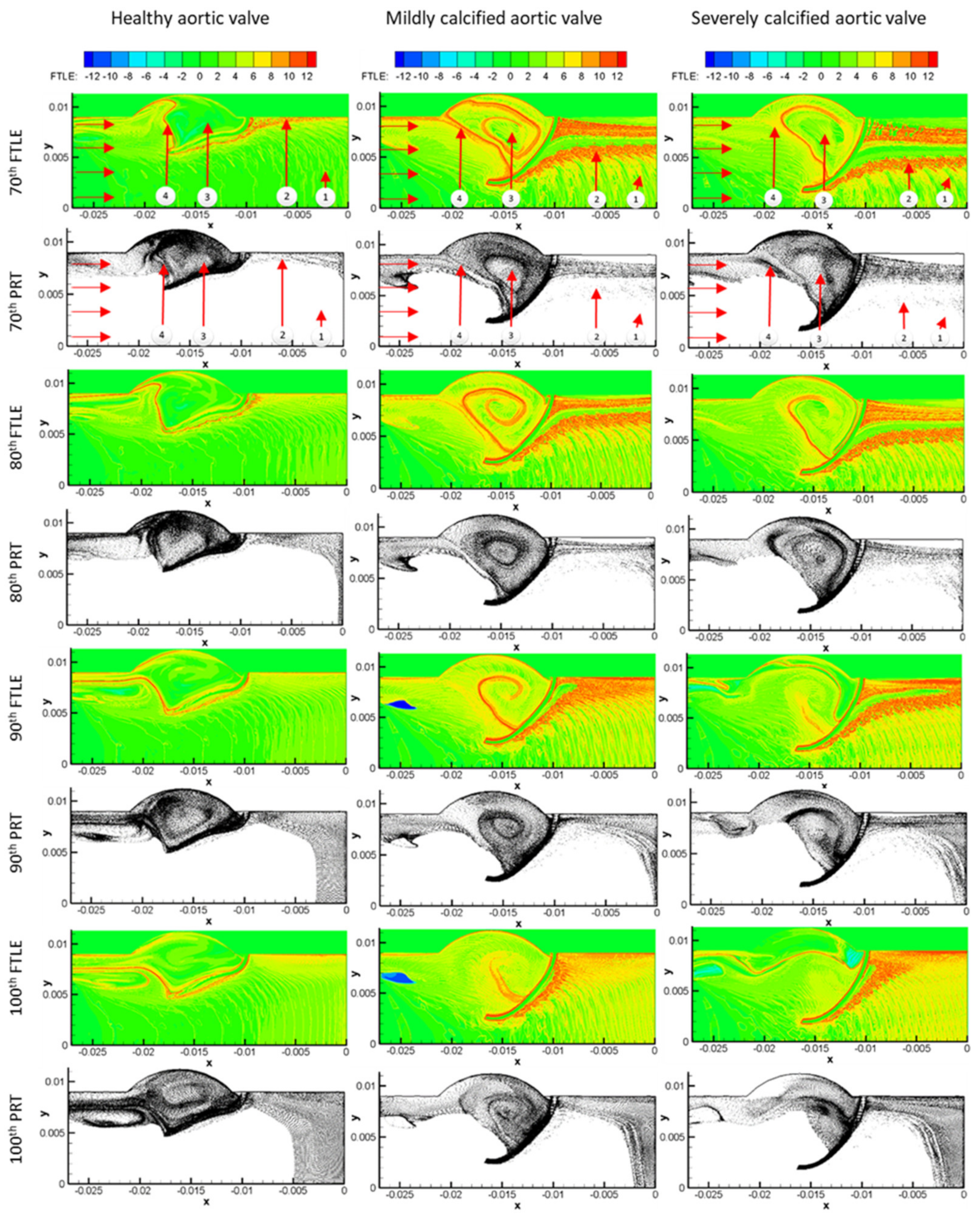
3.2. FTLE Analysis Results

In this study, FTLE analyses were performed for a total of a 1 s cardiac cycle as a result of 400 time steps, each of which took 0.0025 s. FTLE fields can be obtained in two different ways as backward and forward FTLE fields. The backward FTLE velocity vectors are integrated backward in time to form an unstable manifold, while the forward FTLE velocity vectors are integrated forward in time to create a stable manifold. Specifically, backward and forward FTLE fields in the present study were computed by taking integrals of velocity vectors in the backward direction, starting from 1 s to 0 s, and in the forward direction starting from 0 s to 1 s. As a result, the first time step in the normal flow corresponded to the 400th time step in the backward FTLE analysis, since the calculations were made from the last step in the backward FTLE analysis to the first step in the direction of the inlet boundary [51]. To be more specific, backward FTLE analysis could provide information about the future of the fluid flow while showing the flow structures and boundary regions formed by the flow that passed through the valve from the last time step to the first time step.
On the other hand, the 330th to 300th time step in the backward FTLE analysis corresponded to the 70th and 100th time periods in the forward FTLE analysis. Moreover, the forward FTLE analyses were resolved simultaneously with the normal flow time; that is, the analyses used the velocity vectors in the forward time steps starting from the 70th to the 80th time step. It should also be noted that the flow particles in the forward FTLE analysis did not enter the aortic valve, and the flow inside was pulled out from the computational domain. It can also be thought that this happened by reversing the direction of all vectors that made up the flow. For this reason, the direction of the flow moved from left to right in the forward FTLE analysis results. Therefore, the forward FTLE provided information about the flow before the fluid started to move. For example, in the backward FTLE analysis results, the flow structure information passing through the valve at later times could be obtained, while forward FTLE analysis could provide the flow at the earlier times that would eventually enter the valve later.
Figure 4 shows the results of the time evolution of the instantaneous backward FTLE analysis for healthy, mildly calcified, and severely calcified aortic valves. In the FTLE analysis, the velocity and position data were obtained between the 300th and 330th time steps. This covered the duration when the aortic valve began to close from the maximum opening. This analysis was useful to examine the effect of the movements performed by the aortic valve leaflets during the opening–closing process and the LCS regions formed due to these movements. In these graphs, the FTLEs are color-coded, and red lines indicate material line structures in which fluid particles could not cross these red lines during fluid flow. In the 300th FTLE field, the red arrows show the direction and aortic valve openings of the blood flow entering the valve, while the aortic valve openings were calculated as 9.50 mm, 4.85 mm, and 3.70 mm for the healthy, mildly calcified, and severely calcified aortic valves, respectively. These effective orifice areas matched well with the simulation results. Green, blue, purple, and black arrows show blood flow in different flow regions. When these arrows are examined, it should be understood that arrows of the same color point to similar flow regions for the healthy, mildly calcified, and severely calcified valves.
The region indicated by the number 1 arrow in the 300th FTLE, also marked by the red FTLE lines starting from the end of the valves and continuing toward the exit, shows the blood flow that passed the valve and went directly to the exit. While the 300th FTLE field provides information about flow regime and boundaries, the PRT result for the same time step reveals the amount of fluid particles past the aortic valve and residence time in the flow domain. When the number 1 arrow in the healthy valve is examined, the blood flow through the valve becomes laminar because the healthy valve was sufficiently opened by decreasing flow velocity at that section, while the blood flow velocity through the valve had to increase due to reduced area at the valve to ensure the conservation of mass for the mildly and severely calcified valve cases. Therefore, a fluctuation, namely a turbulent flow (seen by a zigzag path in the 330th to 300th FTLE fields in Figure 4), occurred from the tip of the valve toward the outlet for the calcified valves. The area indicated by arrow number 2 and the arrows in green shows the flow zone that passed right over the aortic valve and entered the region between the valve and the vessel wall.
When the 300th PRT was examined, it was seen that the reverse flow regions above the healthy aortic valve were almost absent or very small. However, these regions were more prominent in mildly and severely calcified valves. In other words, in the severely calcified aortic valve model, the inlet opening of the reverse flow zone was higher than in the mildly calcified valve model; therefore, a greater amount of blood could move above the severely calcified aortic valve than above the mildly calcified valve. The regions indicated by the number 3 arrow in the 300th FTLE field indicate the entrance boundary of the vortex structures formed by the movement of the valves between the top of the valve and the vessel wall, and the arrows in black indicate the movement of the vortex structures. When looking at area number 3 in the 300th PRT, it was observed that the vortex formed between the valve and the wall could not be fed because the entrance between the valve and the wall was partially closed. Finally, the FTLE lines formed by the vortex in the mildly and severely calcified aortic valve were more pronounced than in the healthy one, which showed that the reverse blood flow, indicated by the green arrows entering this region, accelerated the vortex.
Starting from the first time step, backward FTLE PRT analyses were performed by adding massless particles from the inlet to a solution domain every 10 time steps. The reason for massless particles to be dispatched every 10 time steps was to better examine and understand the FTLE regions formed between the valve and the vessel wall. In summary, 104,291 massless particles were released to the solution domain from the first time step. Then, 104,291 particles were continued to be added to the solution domain in the same manner every 10 time steps. Table 1 shows the number of particles added and remaining during the FTLE analysis for healthy, mildly calcified, and severely calcified valves. When all cases were examined, particles accumulated from less to more in the healthy, mildly calcified, and severely calcified aortic valve models. The low number of particles indicated that the residence time (RT) was small, and the valve could be sufficiently opened to allow normal blood flow. When the number of particles in the healthy valve model at the 300th step was taken as reference, 1.59 and 1.74 times more particles accumulated in the mildly and severely calcified valves compared to the healthy valve, respectively.
Figure 5 shows the results of the forward FTLE and PRT analyses for the healthy, mildly calcified, and severely calcified aortic valves. The forward FTLE and PRT analyses were the results of the LCS analysis obtained by pulling back the velocity vectors obtained as a result of CFD analysis starting from the last time period. In other words, the forward FTLE and PRT analyses were obtained by drawing the fluid velocity vectors from the outlet to inlet direction starting from the last time step. It was also noted that the result of the 300th time-step analysis in the backward FTLE corresponded to the 100th time step in the forward FTLE. The regions between the inlet boundary in the 70th FTLE field and the aortic valve entrance, surrounded by red FTLE borders starting from the tip of the valve and continuing towards the inlet boundary region (shown with area number 1), indicated the volume of flow that could enter the valve.
The 70th time step in the forward FTLE field shows the instant when the valve opening was around the maximum state for all three studied cases. When these results were examined, it was observed that almost all of the inlet volume in the healthy valve could pass the aortic valve. It was noticed that the flow accumulated between the vessel wall and the red FTLE line indicated by arrow number 2, since the entire volume of the flow could not exceed the valve in the mildly and severely calcified valve models. When regions 1 and 2 were examined together, it was also noted that the flow was laminar in the healthy valve model, whereas the blood velocity reached high speeds at the valve exit of mildly and severely calcified aortic valve cases to satisfy mass conservation, causing fluctuating behavior (the zigzag path in the 330th to 300th FTLE fields in Figure 4) at the downstream.
The directions of the vortex structures formed in the regions indicated by the number 3 arrow in the 70th FTLE field were the opposite of the vortex structures formed in the backward analysis. In other words, the vortex in the backward FTLE analysis results was counterclockwise, while the vortex in the forward FTLE analysis was clockwise. This was because the backward FTLE analysis flow passed the valve from right to left. In the forward FTLE analysis, since the flow was moved from left to right; that is, backwards, the vectors appeared to be in the opposite direction. When the region indicated by the number 3 arrow in the 70th FTLE field was examined, it was observed that the vortex structure did not form yet in this region for the healthy aortic valve. On the other hand, the formation of this structure had been completed for the mildly calcified valve, while this structure had continued to occur for the severely calcified valve model.
The region indicated by arrow number 4 on the 70th FTLE field shows the boundary region that separated the area between the valve and the vessel wall from the mainstream. Since this region was completely closed for the healthy valve, the area indicated by arrow 3 was separated from the other regions, and the vortex structure could not be formed due to the absence of a continuous flow to this area (i.e., the region indicated by the arrow 3). This area in the healthy valve was more stagnant compared to the mildly and severely calcified aortic valves. It was seen that this zone was partially closed in the mildly calcified valve; however, the flow that entered the area indicated by number 3 previously formed the vortex structure due to the late closure of the area represented by number 4 in the 70th FTLE field. When the hemodynamics in the mildly calcified valve was compared with the healthy valve, the high kinetic energy flow in the region indicated by number 3 of the mildly calcified valve caused elongation in the length of the forming vortex.
Since the entrance to the region represented by number 4 of the severely calcified aortic valve was not closed, this was the continuous flow coming into this region, as shown in the 70th FTLE field. The vortex structure formed in the severely calcified valve was shorter than the mildly calcified valve, since region number 3 could not reach stagnation for the severely calcified aortic valve. A red-colored manifold did not form in the region indicated by the number 3 in the healthy valve model in Figure 5, where the forward FTLE field results are presented, which indicated that fluid flow was stationary (no vortex formation). This is also supported by the results of the backward FTLE field because the blood flow at the back of the healthy valve was interrupted, and the blood flow in this region was slow. On the other hand, when the number 3 region was examined in the mildly and severely calcified valve models, it was observed that the blood flow was fast behind the valve, and the vortex was formed by the valve movement. Both backward and forward FTLE field results clearly revealed the vortex formation in the mildly and severely calcified valve models with red LCS lines. In addition, when the severely and mildly calcified valve models were compared within themselves, the number 4 line on the mildly calcified model prevented the flow that tended to enter the number 3 field. However, since line number 4 was not fully a material line (i.e., red-colored lines in FTLE fields generally behaved as a material line) in the severely calcified valve model, it was understood that there was still blood flow to region 3. Therefore, flow in the number 3 area in the severely calcified model was more mobile than the flow in the same area in other models. When the PRT fields were examined, high-density particles were represented by a stagnant flow, while low-density particles were indicated by the presence of mobile flow. Thus, PRT areas could show us the stagnant and moving flow areas between the aortic valve and the vessel wall, and the changes in these areas could be better understood using the PRT results.

4. Discussion

One of the most difficult biomedical problems is the modeling of an aortic valve. Here, while pressure and flow generated by the left ventricle deformed and moved the valve leaflets, the leaflets swept inside the flow domain, generating complex flow movements. During disease, valve leaflets become stiff and cannot open and close efficiently. Such a nonfunctioning valve disturbs flow, as well as mass transport, through the valve.
Computational modeling provides valuable information in cardiovascular flows. While the Eulerian approach provides instantaneous flow information, paths of the fluid particles can be tracked and analyzed in the Lagrangian method. LCS can demonstrate detailed flow analysis by merging flow velocities in backward and forward directions. Particles’ future locations also can be determined from backward FTLE fields when their initial positions are provided. Similarly, fluid particles’ initial positions (i.e., time = 0) can also be identified from forward FTLE fields once the fluid particles’ velocities are known at later times. Formation of flow structures and evolution of circulation zones at the valve site can be clearly identified for healthy and calcified aortic valves in FTLE fields. Furthermore, FTLE fields obtained in the present study only used velocity vector fields of the CFD model without the aortic valve shape and location information. Therefore, LCS is a very powerful technique to investigate flow dynamics through a diseased aortic valve.
LCS was utilized for aortic valve modeling previously by us and others [30]. Current work advanced this approach by incorporating 3D FSI modeling and analysis of PRT fields. In the present study, to characterize flow dynamics through the aortic valve, the LCS technique was employed in Eulerian velocity vectors retrieved from the CFD model to obtain backward FTLE, forward FTLE, and PRT fields at the aortic valve site. Red-colored lines in FTLE fields indicating material lines illustrated the formation of vortex structures around the leaflet and opening distance of the aortic valve for healthy, mildly, and severely calcified leaflet models. Once opening at the aortic valve could be accurately determined from backward FTLE field results, it was noted that the opening of the severely calcified valve was nearly 40% of the healthy valve’s opening. This implies that velocity at the severely calcified valve can be 1.7 times higher than the velocity at the healthy valve yielding fluctuations and transition to turbulent flow behavior. These types of fluctuations can cause wear on already-calcified aortic valves; therefore, amplitude and direction of fluctuations obtained from FTLE fields can be used to determine the life of a patient’s aortic valve. Furthermore, PRT fields providing particle movements can identify locations of dense particle regions at the valve site. Particle movements and eventually accumulations of particles on the leaflet region can provide information on how and why pressure variation occurs by identifying the physics of fluid motion for aortic leaflets. A change in particle movements for healthy, mildly calcified, and severely calcified leaflets can be used to understand how calcification affects blood flow at the region between the aortic valve and vessel. Distinct flow regions characterized by vortices were easily identified with LCS in the analysis (Figure 4). Decreased leaflet movement due to calcification resulted in backflow regions within the sinuses, which was not present in healthy leaflets. Deteriorated leaflet movements also caused a decreased mass flow rate, as seen in Table 1. On the other hand, a difference in flow structures of mildly and severely calcified leaflets was identified, and particle density provided stagnant and mobile fluid flow zones at the aortic valve site (Figure 5).
In conclusion, the LCS technique, once used with the Eulerian approach, is a very powerful approach to examine unsteady flow phenomena. In this work, we applied this approach to investigate disturbed flow dynamics in aortic valve disease. We were able to identify distinct stagnant and circulatory flow regions, which would not be possible to identify with pure Lagrangian or Eulerian approaches. Decreased fluid transports were also revealed with calcified leaflets.

5. Limitations

In this study, we employed the LCS technique using FTLE computations and Lagrangian PRT analysis both in forward and backward directions to investigate the complex flow regions in the healthy and calcified aortic valves. Due to several limitations in our model, further improvements are suggested for future studies. The 3D geometric model of the aortic valve can be improved by using multiple layers of patient-specific images for a better resolution. The leaflets can be modeled as multilayered structures with hyperelastic and anisotropic material properties [54]. Spatially heterogeneous calcific deposits can also be modeled with the help of medical imaging techniques [9,55]. The blood can be modeled as a non-Newtonian fluid with varying viscosity depending on the shear environment [56]. The aortic root and aortic sinuses can be modeled as deformable structures with elastic material properties. Nevertheless, the obtained results provided insight into understanding alterations in the aortic valve hemodynamics due to leaflet calcifications.

Author Contributions

Conceptualization, H.C.Y. and A.B.O.; methodology, O.M., H.E.S., H.C.Y. and A.B.O.; software, O.M. and H.E.S.; validation, O.M., H.E.S., H.C.Y. and A.B.O.; formal analysis, O.M. and H.E.S.; investigation, O.M., H.E.S., H.C.Y. and A.B.O.; resources, H.C.Y. and A.B.O.; data curation, O.M. and H.E.S.; writing—original draft preparation, O.M. and H.E.S.; writing—review and editing, H.C.Y. and A.B.O.; visualization, O.M. and H.E.S.; supervision, H.C.Y. and A.B.O.; project administration, H.C.Y. and A.B.O.; funding acquisition, H.C.Y. All authors have read and agreed to the published version of the manuscript.

Funding

This study was funded by the Qatar National Research Fund (QNRF), National Priority Research Program (NPRP13S-0108-200024) to H.C.Y. and O.M.; and the Qatar University International Research Collaboration Co-Fund (IRCC) program (IRCC-2020-002) to H.C.Y. The publication of this article was funded by the Qatar National Library (QNL).

Institutional Review Board Statement

The study was conducted according to the guidelines of the Declaration of Helsinki, and approved by the Ethics Committee of ISTANBUL UNIVERSITY CERRAHPASA MEDICAL SCHOOL, TURKEY (protocol code: B.30.2.İST.0.30.90.00/18991, date of approval: 3 July 2012).

Informed Consent Statement

Informed consent was obtained from all subjects involved in the study.

Data Availability Statement

Not applicable.

Conflicts of Interest

The authors declare no conflict of interest.

References

  1. Gould, S.T.; Srigunapalan, S.; Simmons, C.A.; Anseth, K.S. Hemodynamic and Cellular Response Feedback in Calcific Aortic Valve Disease. Circ. Res. 2013, 113, 186–197. [Google Scholar] [CrossRef] [PubMed] [Green Version]
  2. Stewart, B.F.; Siscovick, D.; Lind, B.K.; Gardin, J.M.; Gottdiener, J.S.; Smith, V.E.; Kitzman, D.W.; Otto, C.M. Clinical Factors Associated with Calcific Aortic Valve Disease. J. Am. Coll. Cardiol. 1997, 29, 630–634. [Google Scholar] [CrossRef] [Green Version]
  3. Halevi, R.; Hamdan, A.; Marom, G.; Mega, M.; Raanani, E.; Haj-Ali, R. Progressive Aortic Valve Calcification: Three-Dimensional Visualization and Biomechanical Analysis. J. Biomech. 2015, 48, 489–497. [Google Scholar] [CrossRef] [PubMed]
  4. De Hart, J.; Peters, G.W.M.; Schreurs, P.J.G.; Baaijens, F.P.T. A Two-Dimensional Fluid-Structure Interaction Model of the Aortic Value. J. Biomech. 2000, 33, 1079–1088. [Google Scholar] [CrossRef]
  5. Amindari, A.; Saltik, L.; Kirkkopru, K.; Yacoub, M.; Yalcin, H.C. Assessment of Calcified Aortic Valve Leaflet Deformations and Blood Flow Dynamics Using Fluid-Structure Interaction Modeling. Inform. Med. Unlocked 2017, 9, 191–199. [Google Scholar] [CrossRef]
  6. De Hart, J.; Peters, G.W.M.; Schreurs, P.J.G.; Baaijens, F.P.T. A Three-Dimensional Computational Analysis of Fluid—Structure Interaction in the Aortic Valve. J. Biomech. 2003, 36, 103–112. [Google Scholar] [CrossRef]
  7. Spühler, J.H.; Jansson, J.; Jansson, N.; Hoffman, J. 3D Fluid–Structure Interaction Simulation of Aortic Valves Using a Unified Continuum ALE FEM Model. Front. Physiol. 2018, 9, 363. [Google Scholar] [CrossRef] [PubMed] [Green Version]
  8. Mao, W.; Caballero, A.; McKay, R.; Primiano, C.; Sun, W. Fully-Coupled Fluid-Structure Interaction Simulation of the Aortic and Mitral Valves in a Realistic 3D Left Ventricle Model. PLoS ONE 2017, 12, e018472. [Google Scholar] [CrossRef] [Green Version]
  9. Halevi, R.; Hamdan, A.; Marom, G.; Lavon, K.; Ben-Zekry, S.; Raanani, E.; Bluestein, D.; Haj-Ali, R. Fluid–Structure Interaction Modeling of Calcific Aortic Valve Disease Using Patient-Specific Three-Dimensional Calcification Scans. Med. Biol. Eng. Comput. 2016, 54, 1683–1694. [Google Scholar] [CrossRef]
  10. Haj-Ali, R.; Dasi, L.P.; Kim, H.S.; Choi, J.; Leo, H.W.; Yoganathan, A.P. Structural Simulations of Prosthetic Tri-Leaflet Aortic Heart Valves. J. Biomech. 2008, 41, 1510–1519. [Google Scholar] [CrossRef]
  11. Dumont, K.; Vierendeels, J.; Kaminsky, R.; Van Nooten, G.; Verdonck, P.; Bluestein, D. Comparison of the Hemodynamic and Thrombogenic Performance of Two Bileaflet Mechanical Heart Valves Using a CFD/FSI Model. J. Biomech. Eng. 2007, 129, 558–565. [Google Scholar] [CrossRef] [Green Version]
  12. Bavo, A.M.; Rocatello, G.; Iannaccone, F.; Degroote, J.; Vierendeels, J.; Segers, P. Fluid-Structure Interaction Simulation of Prosthetic Aortic Valves: Comparison between Immersed Boundary and Arbitrary Lagrangian-Eulerian Techniques for the Mesh Representation. PLoS ONE 2016, 11, e0154517. [Google Scholar] [CrossRef] [Green Version]
  13. Borazjani, I. Fluid–Structure Interaction, Immersed Boundary-Finite Element Method Simulations of Bio-Prosthetic Heart Valves. Comput. Methods Appl. Mech. Eng. 2013, 257, 103–116. [Google Scholar] [CrossRef]
  14. Chandran, K.B.; Vigmostad, S.C. Patient-Specific Bicuspid Valve Dynamics: Overview of Methods and Challenges. J. Biomech. 2013, 46, 208–216. [Google Scholar] [CrossRef] [PubMed] [Green Version]
  15. Conti, C.A.; Votta, E.; Della Corte, A.; Del Viscovo, L.; Bancone, C.; Cotrufo, M.; Redaelli, A. Dynamic Finite Element Analysis of the Aortic Root from MRI-Derived Parameters. Med. Eng. Phys. 2010, 32, 212–221. [Google Scholar] [CrossRef]
  16. Cao, K.; BukaČ, M.; Sucosky, P. Three-Dimensional Macro-Scale Assessment of Regional and Temporal Wall Shear Stress Characteristics on Aortic Valve Leaflets. Comput. Methods Biomech. Biomed. Eng. 2016, 19, 603–613. [Google Scholar] [CrossRef]
  17. Cao, K.; Sucosky, P. Computational Comparison of Regional Stress and Deformation Characteristics in Tricuspid and Bicuspid Aortic Valve Leaflets. Int. J. Numer. Method. Biomed. Eng. 2017, 33, e02798. [Google Scholar] [CrossRef]
  18. Gilmanov, A.; Sotiropoulos, F. Comparative Hemodynamics in an Aorta with Bicuspid and Trileaflet Valves. Theor. Comput. Fluid Dyn. 2016, 30, 67–85. [Google Scholar] [CrossRef]
  19. Weinberg, E.J.; Kaazempur Mofrad, M.R. A Multiscale Computational Comparison of the Bicuspid and Tricuspid Aortic Valves in Relation to Calcific Aortic Stenosis. J. Biomech. 2008, 41, 3482–3487. [Google Scholar] [CrossRef] [PubMed]
  20. Chandra, S.; Rajamannan, N.M.; Sucosky, P. Computational Assessment of Bicuspid Aortic Valve Wall-Shear Stress: Implications for Calcific Aortic Valve Disease. Biomech. Model. Mechanobiol. 2012, 11, 1085–1096. [Google Scholar] [CrossRef]
  21. Kuan, M.Y.S.; Espino, D.M. Systolic Fluid–Structure Interaction Model of the Congenitally Bicuspid Aortic Valve: Assessment of Modelling Requirements. Comput. Methods Biomech. Biomed. Eng. 2015, 18, 1305–1320. [Google Scholar] [CrossRef] [PubMed]
  22. Marom, G.; Peleg, M.; Halevi, R.; Rosenfeld, M.; Raanani, E.; Hamdan, A.; Haj-Ali, R. Fluid-Structure Interaction Model of Aortic Valve with Porcine-Specific Collagen Fiber Alignment in the Cusps. J. Biomech. Eng. 2013, 135, 101001–101006. [Google Scholar] [CrossRef] [Green Version]
  23. Grande, K.J.; Cochran, R.P.; Reinhall, P.G.; Kunzelma, K.S. Stress Variations in the Human Aortic Root and Valve: The Role of Anatomic Asymmetry. Ann. Biomed. Eng. 1998, 26, 534–545. [Google Scholar] [CrossRef]
  24. Votta, E.; Le, T.B.; Stevanella, M.; Fusini, L.; Caiani, E.G.; Redaelli, A.; Sotiropoulos, F. Toward Patient-Specific Simulations of Cardiac Valves: State-of-the-Art and Future Directions. J. Biomech. 2013, 46, 217–228. [Google Scholar] [CrossRef] [PubMed] [Green Version]
  25. Katayama, S.; Umetani, N.; Sugiura, S.; Hisada, T. The Sinus of Valsalva Relieves Abnormal Stress on Aortic Valve Leaflets by Facilitating Smooth Closure. J. Thorac. Cardiovasc. Surg. 2008, 136, 1528–1535.e1. [Google Scholar] [CrossRef] [Green Version]
  26. Balachandran, K.; Sucosky, P.; Yoganathan, A.P. Hemodynamics and Mechanobiology of Aortic Valve Inflammation and Calcification. Int. J. Inflamm. 2011, 2011, 263870. [Google Scholar] [CrossRef] [PubMed] [Green Version]
  27. Hutcheson, J.D.; Goettsch, C.; Rogers, M.A.; Aikawa, E. Revisiting Cardiovascular Calcification: A Multifaceted Disease Requiring a Multidisciplinary Approach. Semin. Cell Dev. Biol. 2015, 46, 68–77. [Google Scholar] [CrossRef] [PubMed] [Green Version]
  28. Seaman, C.; McNally, A.; Biddle, S.; Jankowski, L.; Sucosky, P. Generation of Simulated Calcific Lesions in Valve Leaflets for Flow Studies. J. Heart Valve Dis. 2015, 24, 115–125. [Google Scholar] [PubMed]
  29. Arjunon, S.; Rathan, S.; Jo, H.; Yoganathan, A.P. Aortic Valve: Mechanical Environment and Mechanobiology. Ann. Biomed. Eng. 2013, 41, 1331–1346. [Google Scholar] [CrossRef] [PubMed] [Green Version]
  30. Olcay, A.B.; Amindari, A.; Kirkkopru, K.; Yalcin, H.C. Characterization of Disturbed Hemodynamics Due to Stenosed Aortic Jets with a Lagrangian Coherent Structures Technique. J. Appl. Fluid Mech. 2018, 11, 375–384. [Google Scholar] [CrossRef]
  31. Shadden, S.C.; Astorino, M.; Gerbeau, J.-F. Computational Analysis of an Aortic Valve Jet with Lagrangian Coherent Structures. Chaos Interdiscip. J. Nonlinear Sci. 2010, 20, 017512. [Google Scholar] [CrossRef] [Green Version]
  32. May-Newman, K.; Vu, V.; Herold, B. Modeling the Link between Left Ventricular Flow and Thromboembolic Risk Using Lagrangian Coherent Structures. Fluids 2016, 1, 38. [Google Scholar] [CrossRef]
  33. Green, M.A.; Rowley, C.W.; Smits, A.J. Using Hyperbolic Lagrangian Coherent Structures to Investigate Vortices in Bioinspired Fluid Flows. Chaos 2010, 20, 017510. [Google Scholar] [CrossRef] [Green Version]
  34. Shadden, S.C.; Arzani, A. Lagrangian Postprocessing of Computational Hemodynamics. Ann. Biomed. Eng. 2015, 43, 41–58. [Google Scholar] [CrossRef]
  35. Olcay, A.B.; Krueger, P.S. Measurement of Ambient Fluid Entrainment during Laminar Vortex Ring Formation. Exp. Fluids 2008, 44, 235–247. [Google Scholar] [CrossRef]
  36. Olcay, A.B.; Pottebaum, T.S.; Krueger, P.S. Sensitivity of Lagrangian Coherent Structure Identification to Flow Field Resolution and Random Errors. Chaos 2010, 20, 017506. [Google Scholar] [CrossRef] [PubMed]
  37. Olcay, A.B.; Krueger, P.S. Momentum Evolution of Ejected and Entrained Fluid during Laminar Vortex Ring Formation. Theor. Comput. Fluid Dyn. 2010, 24, 465–482. [Google Scholar] [CrossRef]
  38. Olcay, A.B. Investigation of a Wake Formation for Flow over a Cylinder Using Lagrangian Coherent Structures. Prog. Comput. Fluid Dyn. 2016, 16, 126–130. [Google Scholar] [CrossRef]
  39. Mutlu, O.; Olcay, A.B.; Bilgin, C.; Hakyemez, B. Evaluating the Effectiveness of 2 Different Flow Diverter Stents Based on the Stagnation Region Formation in an Aneurysm Sac Using Lagrangian Coherent Structure. World Neurosurg. 2019, 127, e727–e737. [Google Scholar] [CrossRef] [PubMed]
  40. Mutlu, O.; Olcay, A.B.; Bilgin, C.; Hakyemez, B. Evaluating the Effect of the Number of Wire of Flow Diverter Stents on the Nonstagnated Region Formation in an Aneurysm Sac Using Lagrangian Coherent Structure and Hyperbolic Time Analysis. World Neurosurg. 2020, 133, e666–e682. [Google Scholar] [CrossRef] [PubMed]
  41. Mutlu, O.; Olcay, A.B.; Bilgin, C.; Hakyemez, B. Understanding the Effect of Effective Metal Surface Area of Flow Diverter Stent’s on the Patient-Specific Intracranial Aneurysm Numerical Model Using Lagrangian Coherent Structures. J. Clin. Neurosci. 2020, 133, e666–e682. [Google Scholar] [CrossRef]
  42. Chester, A.H.; El-Hamamsy, I.; Butcher, J.T.; Latif, N.; Bertazzo, S.; Yacoub, M.H. The Living Aortic Valve: From Molecules to Function. Glob. Cardiol. Sci. Pract. 2014, 2014, 11. [Google Scholar] [CrossRef] [Green Version]
  43. Girfoglio, M.; Quaini, A.; Rozza, G. A Finite Volume Approximation of the Navier-Stokes Equations with Nonlinear Filtering Stabilization. Comput. Fluids 2019, 187, 27–45. [Google Scholar] [CrossRef] [Green Version]
  44. Frolov, S.V.; Sindeev, S.V.; Lischouk, V.A.; Gazizova, D.S.; Liepsch, D.; Balasso, A. A Lumped Parameter Model of Cardiovascular System with Pulsating Heart for Diagnostic Studies. J. Mech. Med. Biol. 2017, 17, 1750056. [Google Scholar] [CrossRef]
  45. Young, D.F. Fluid Mechanics of Arterial Stenoses. J. Biomech. Eng. 1979, 101, 157–175. [Google Scholar] [CrossRef]
  46. Meslem, A.; Bode, F.; Croitoru, C.; Nastase, I. Comparison of Turbulence Models in Simulating Jet Flow from a Cross-Shaped Orifice. Eur. J. Mech. B Fluids 2014, 44, 100–120. [Google Scholar] [CrossRef]
  47. Benra, F.K.; Dohmen, H.J.; Pei, J.; Schuster, S.; Wan, B. A Comparison of One-Way and Two-Way Coupling Methods for Numerical Analysis of Fluid-Structure Interactions. J. Appl. Math. 2011, 2011, 853560. [Google Scholar] [CrossRef]
  48. Salman, H.E.; Ramazanli, B.; Yavuz, M.M.; Yalcin, H.C. Biomechanical Investigation of Disturbed Hemodynamics-Induced Tissue Degeneration in Abdominal Aortic Aneurysms Using Computational and Experimental Techniques. Front. Bioeng. Biotechnol. 2019, 7, 111. [Google Scholar] [CrossRef]
  49. Bathe, K.J.; Zhang, H.; Ji, S. Finite Element Analysis of Fluid Flows Fully Coupled with Structural Interactions. Comput. Struct. 1999, 72, 1–16. [Google Scholar] [CrossRef] [Green Version]
  50. Haller, G. Distinguished Material Surfaces and Coherent Structures in Three-Dimensional Fluid Flows. Phys. D Nonlinear Phenom. 2001, 149, 248–277. [Google Scholar] [CrossRef] [Green Version]
  51. Shadden, S.C.; Lekien, F.; Marsden, J.E. Definition and Properties of Lagrangian Coherent Structures from Finite-Time Lyapunov Exponents in Two-Dimensional Aperiodic Flows. Phys. D Nonlinear Phenom. 2005, 212, 271–304. [Google Scholar] [CrossRef]
  52. Lekien, F.; Shadden, S.C.; Marsden, J.E. Lagrangian Coherent Structures in N-Dimensional Systems. J. Math. Phys. 2007, 48, 065404. [Google Scholar] [CrossRef]
  53. Shadden, S.C.; Taylor, C.A. Characterization of Coherent Structures in the Cardiovascular System. Ann. Biomed. Eng. 2008, 36, 1152–1162. [Google Scholar] [CrossRef] [PubMed]
  54. Weinberg, E.J.; Mofrad, M.R.K. Three-Dimensional, Multiscale Simulations of the Human Aortic Valve. Cardiovasc. Eng. 2007, 7, 140–155. [Google Scholar] [CrossRef]
  55. Weska, R.F.; Aimoli, C.G.; Nogueira, G.M.; Leirner, A.A.; Maizato, M.J.S.; Higa, O.Z.; Polakievicz, B.; Pitombo, R.N.M.; Beppu, M.M. Natural and Prosthetic Heart Valve Calcification: Morphology and Chemical Composition Characterization. Artif. Organs 2010, 34, 311–318. [Google Scholar] [CrossRef] [PubMed]
  56. Nandy, S.; Tarbell, J.M. Flush Mounted Hot Film Anemometer Measurement of Wall Shear Stress Distal to a Tri-Leaflet Valve for Newtonian and Non-Newtonian Blood Analog Fluids. Biorheology 1987, 24, 483–500. [Google Scholar] [CrossRef]
Figure 1. (a) 3D aortic valve model. The grey surface is the cross-sectional plane in the longitudinal direction. The arrows show the direction of flow at the inlet and outlet. (b) 2D view of the cross-sectional plane. Only the top half of the model is shown due to the symmetry. The dashed line represents the symmetry line. (c) Boundary conditions shown on the cross-sectional plane. (d) Transient inlet velocity profile of the blood flow. (e) Mesh of the fluid domain. (f) Mesh of the solid domain.
Fluids 06 00203 g001aFluids 06 00203 g001b
Figure 2. Velocity streamlines on the 3D aortic valve model. The configuration of the maximum valve opening for the healthy aortic valve is given at the bottom of the figure.
Fluids 06 00203 g002
Figure 3. Pressure on the selected fluid particles for healthy, mildly calcified, and severely calcified aortic valves. The results are shown on the top half of the cross-sectional plane given in Figure 1. The flow was from right to left. The values presented are pressures relative to the valve outlet. The pressure was set to zero at the outlet boundary.
Fluids 06 00203 g003
Figure 4. Backward finite-time Lyapunov exponent (FTLE) field plots of healthy (first column), mildly calcified (second column), and severely calcified (third column) aortic valves.
Fluids 06 00203 g004
Figure 5. Forward finite-time Lyapunov exponent (FTLE) field plots of healthy (first column), mildly calcified (second column), and severely calcified (third column) aortic valves.
Fluids 06 00203 g005
Table 1. The number of particles in the solution domain for the backward FTLE PRT analysis.
Healthy Aortic ValveMildly Calcified Aortic ValveSeverely Calcified Aortic Valve
400th step (added for the first time)104,291104,291104,291
339th step (Total with readded particles)261,418398,350434,337
330th step (remaining particles)153,900285,259325,046
329th step (total with readded particles)254,945382,472421,736
320th step (remaining particles)155,146268,018305,521
319th step (total with re-added particles)255,743367,599403,394
310th step (remaining particles)165,389276,347309,397
309th step (total with readded particles)263,070376,494407977
300th step (remaining particles)185,322295,500323,787
Publisher’s Note: MDPI stays neutral with regard to jurisdictional claims in published maps and institutional affiliations.

