
Equation of State’s Crossover Enhancement of Pseudopotential Lattice Boltzmann Modeling of CO2 Flow in Homogeneous Porous Media


Abstract
:1. Introduction
2. Methodology
2.1. General Lattice Boltzmann Model
2.2. Pseudopotential Lattice Boltzmann Model
2.3. Crossover Peng–Robinson EoS
3. Results
3.1. Multicomponent System
3.2. Contact Angle Test
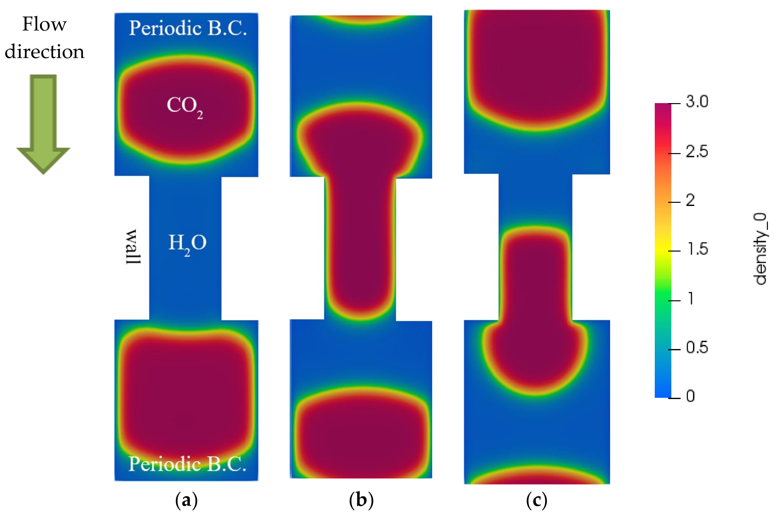
3.3. Penetration Process in 2D Narrow Channel
3.4. Penetration Process in the 2D Pore Network
4. Discussion and Concluding Remarks
Author Contributions
Funding
Institutional Review Board Statement
Informed Consent Statement
Data Availability Statement
Acknowledgments
Conflicts of Interest
Abbreviations
| χ | Local value of the mass fraction |
| Non-dimensional Helmholtz’s free energy per mole | |
| Critical volume | |
| Gas constant | |
| Dimensionless temperature | |
| Critical temperature | |
| Critical compressibility factor | |
| Dimensionless coefficients for Helmholtz free energy for the PT equation of state | |
| Critical exponent | |
| Coefficients of Landau expansion | |
| Ginzburg number | |
| Coefficients of rectilinear diameter | |
| , | Critical exponents |
| Body force |
References
- Polikhronidi, N.; Batyrova, R.; Aliev, A.; Abdulagatov, I. Supercritical CO2: Properties and Technological Applications-A Review. J. Therm. Sci. 2019, 28, 394–430. [Google Scholar] [CrossRef]
- Brown, D. A Hot Dry Rock Geothermal Energy Concept Utilizing Supercritical CO2 Instead of Water. In Proceedings of the Twenty-Fifth Workshop on Geothermal Reservoir Engineering, SGP-TR-165, Stanford, CA, USA, 24–26 January 2000. [Google Scholar]
- Holdych, D.J.; Georgiadis, J.G.; Buckius, R.O. Hydrodynamic instabilities of near-critical CO2 flow in microchannels: Lattice Boltzmann simulation. Phys. Fluids 2004, 16, 1791–1802. [Google Scholar] [CrossRef]
- Huai, X.L.; Koyama, S.; Zhao, T.S. An experimental study of flow and heat transfer of supercritical carbon dioxide in multi-port mini channels under cooling conditions. Chem. Eng. Sci. 2005, 60, 3337–3345. [Google Scholar] [CrossRef]
- Pitla, S.S.; Robinson, D.M.; Groll, E.A.; Ramadhyani, S. Heat transfer from supercritical carbon dioxide in tube flow: A critical review. HVACR Res. 1998, 4, 281–301. [Google Scholar] [CrossRef]
- Katopodes, N. Free-Surface Flow. Computational Methods, Butterworth-Heineman, Oxford. 2019. Available online: https://doi.org/10.1016/b978-0-12-815485-4.00002-4 (accessed on 10 January 2021). [CrossRef]
- Osher, S.; Sethian, J.A. Fronts propagating with curvature-dependent speed: Algorithms based on Hamilton-Jacobi formulations. J. Comput. Phys. 1988, 79, 12–49. [Google Scholar] [CrossRef] [Green Version]
- Shan, X.; Chen, H. Lattice Boltzmann model for simulating flows with multiple phases and components. Phys. Rev. E 1993, 47, 1815. [Google Scholar] [CrossRef] [Green Version]
- Yuan, P.; Schaefer, L. Equations of state in a lattice Boltzmann model. Phys. Fluids 2006, 18, 042101. [Google Scholar] [CrossRef]
- Liu, H.; Zhang, Y.; Valocchi, A.J. Lattice Boltzmann simulation of immiscible fluid displacement in porous media: Homogeneous versus heterogeneous pore network. Phys. Fluids 2015, 27, 052103. [Google Scholar] [CrossRef] [Green Version]
- Liu, H.; Valocchi, A.J.; Werth, C.; Kang, Q.; Oostrom, M. Pore-scale simulation of liquid CO2 displacement of water using a two-phase lattice Boltzmann model. Adv. Water Resour. 2014, 73, 144–158. [Google Scholar] [CrossRef] [Green Version]
- Liu, H.; Kang, Q.; Leonardi, C.R.; Schmieschek, S.; Narváez, A.; Jones, B.D.; Williams, J.R.; Valocchi, A.J.; Harting, J. Multiphase lattice Boltzmann simulations for porous media applications: A review. Comput. Geosci. 2016, 20, 777–805. [Google Scholar] [CrossRef] [Green Version]
- Zhao, H.; Ning, Z.; Kang, Q.; Chen, L.; Zhao, T. Relative permeability of two immiscible fluids flowing through porous media determined by lattice Boltzmann method. Int. Commun. Heat Mass Transf. 2017, 85, 53–61. [Google Scholar] [CrossRef]
- Boek, E.S.; Venturoli, M. Lattice-Boltzmann studies of fluid flow in porous media with realistic rock geometries. Comput. Math. Appl. 2010, 59, 2305–2314. [Google Scholar] [CrossRef] [Green Version]
- Stiles, C.D.; Xue, Y. High density ratio lattice Boltzmann method simulations of multicomponent multiphase transport of H2O in air. Comput. Fluids 2016, 131, 81–90. [Google Scholar] [CrossRef]
- Ikeda, M.K.; Rao, P.R.; Schaefer, L.A. A thermal multicomponent lattice Boltzmann model. Comput. Fluids 2014, 101, 250–262. [Google Scholar] [CrossRef]
- Kupershtokh, A.L.; Medvedev, D.A.; Karpov, D.I. On equations of state in a lattice Boltzmann method. Comput. Math. Appl. 2009, 58, 965–974. [Google Scholar] [CrossRef] [Green Version]
- Kiselev, S.B. Cubic Crossover Equation of State. Fluid Phase Equilib. 1998, 147, 7–23. [Google Scholar] [CrossRef]
- Kiselev, S.B.; Ely, J.F. Generalized corresponding states model for bulk and interfacial properties in pure fluids and fluid mixtures. J. Chem. Phys. 2003, 119, 8645–8662. [Google Scholar] [CrossRef] [Green Version]
- Kiselev, S.B.; Ely, J.F. Generalized crossover description of the thermodynamic and transport properties in pure fluids. Fluid Phase Equilib. 2004, 222–223, 149–159. [Google Scholar] [CrossRef]
- Feyzi, F.; Seydi, M.; Alavi, F. Crossover Peng-Robinson equation of state with introduction of a new expression for the crossover function. Fluid Phase Equilib. 2010, 293, 251–260. [Google Scholar] [CrossRef]
- Feyzi, F.; Riazi, M.R.; Shaban, H.I.; Ghotbi, S. Improving cubic equations of state for heavy reservoir fluids and critical region. Chem. Eng. Commun. 1998, 167, 147–166. [Google Scholar] [CrossRef]
- Kabdenova, B.; Rojas-Solórzano, L.R.; Monaco, E. Lattice Boltzmann simulation of near/supercritical CO2 flow featuring a crossover formulation of the equation of state. Comput. Fluids 2020, 216, 104820. [Google Scholar] [CrossRef]
- Atykhan, M.; Kabdenova, B.; Monaco, E.; Rojas-Solórzano, L.R. Modeling Immiscible Fluid Displacement in a Porous Medium Using Lattice Boltzmann Method. Fluids 2021, 6, 89. [Google Scholar] [CrossRef]
- He, X.; Luo, L. Theory of the lattice Boltzmann method: From the Boltzmann equation to the lattice Boltzmann equation. Phys. Rev. E 1997, 56, 6811–6817. [Google Scholar] [CrossRef] [Green Version]
- Huang, H.; Sukop, M.; Lu, X.-Y. Multiphase Lattice Boltzman Methods Theory and Application; John Wiley & Sons, Ltd.: Sussex, UK, 2015. [Google Scholar]
- Martys, N.S.; Chen, H. Simulation of multicomponent fluids in complex three-dimensional geometries by the lattice Boltzmann method. Phys. Rev. E Stat. Phys. Plasmas Fluids Relat. Interdiscip. Top. 1996, 53, 743–750. [Google Scholar] [CrossRef]
- Shan, X. Analysis and reduction of the spurious current in a class of multiphase Lattice Boltzmann models. Phys. Rev. E Stat. Nonlinear Soft Matter Phys. 2006, 73, 6–9. [Google Scholar] [CrossRef]
- Monaco, E.; Brenner, G.; Luo, K.H. Numerical simulation of the collision of two microdroplets with a pseudopotential multiple-relaxation-time lattice Boltzmann model. Microfluid. Nanofluidics 2014, 16, 329–346. [Google Scholar] [CrossRef]
- Guo, Z.; Zheng, C.; Shi, B. Discrete lattice effects on the forcing term in the lattice Boltzmann method. Phys. Rev. E Stat. Phys. Plasmas Fluids Relat. Interdiscip. Top. 2002, 65, 6. [Google Scholar] [CrossRef] [PubMed]
- Landau, L.; Lifshitz, E.M. Statistical Physics; Pergamon Press Ltd.: Headington Hill Hall, Oxford, England, UK, 1980. [Google Scholar]
- Thermophysical Properties of Fluid Systems in NIST Chemistry Webbook, NIST Standard Reference Database No.69, National Institute of Standards and Technology, (n.d.). Available online: https://webbook.nist.gov (accessed on 10 October 2018).
- Li, Q.; Luo, K.H.; Li, X.J. Forcing scheme in pseudopotential lattice Boltzmann model for multiphase flows. Phys. Rev. E Stat. Nonlinear Soft Matter Phys. 2012, 86, 016709. [Google Scholar] [CrossRef] [Green Version]
- Huang, H.; Krafczyk, M.; Lu, X. Forcing term in single-phase and Shan-Chen-type multiphase lattice Boltzmann models. Phys. Rev. E Stat. Nonlinear Soft Matter Phys. 2011, 84, 046710. [Google Scholar] [CrossRef] [PubMed] [Green Version]
- Liu, Y.; Mutailipu, M.; Jiang, L.; Zhao, J.; Song, Y.; Chen, L. Interfacial Tension and Contact Angle Measurements for the Evaluation of CO2-Brine Two-Phase Flow Characteristics in Porous Media. Environ. Prog. Sustain. Energy 2015, 34, 1756–1762. [Google Scholar] [CrossRef]
- Fakhari, A.; Rahimian, M.H. Phase-field modeling by the method of lattice Boltzmann equations. Phys. Rev. E 2010, 81, 036707. [Google Scholar] [CrossRef]
- Suekane, T.; Soukawa, S.; Iwatani, S.; Tsushima, S.; Hirai, S. Behavior of supercritical CO2 injected into porous media containing water. Energy 2005, 30, 2370–2382. [Google Scholar] [CrossRef]
- Swift, M.; Osborn, W.; Yeomans, J. Lattice Boltzmann Simulation of Nonideal Fluids. Phys. Rev. Lett. 1995, 75, 3824–3827. [Google Scholar] [CrossRef] [PubMed] [Green Version]
- Fakhari, A.; Li, Y.; Bolster, D.; Christensen, K.T. A phase-field lattice Boltzmann model for simulating multiphase flows in porous media: Application and comparison to experiments of CO2 sequestration at pore scale. Adv. Water Resour. 2018, 114, 119–134. [Google Scholar] [CrossRef]
- Zou, Q.; He, X. On pressure and velocity flow boundary conditions and bounceback for the lattice Boltzmann BGK model. Phys. Fluids 1997, 9, 1591–1598. [Google Scholar] [CrossRef] [Green Version]
- Fakhari, A.; Rahimian, M. Investigation of deformation and breakup of a moving droplet by the method of lattice Boltzmann equations. Int. J. Numer. Methods Fluids 2009, 64, 827–849. [Google Scholar] [CrossRef]


| Physical Critical Parameters | CO2 | H2O |
|---|---|---|
| Critical shift | ||
| Crossover parameters | ||
| Physical for CO2 | |||
|---|---|---|---|
| 304.1 K | 647.1 K | 0.03428 | 0.07292 |
| θeq | ||
|---|---|---|
| 70° | 0.2 | −0.2 |
| 90° | 0 | 0 |
| 120° | −0.2 | 0.2 |
| 130° | −0.3 | 0.3 |
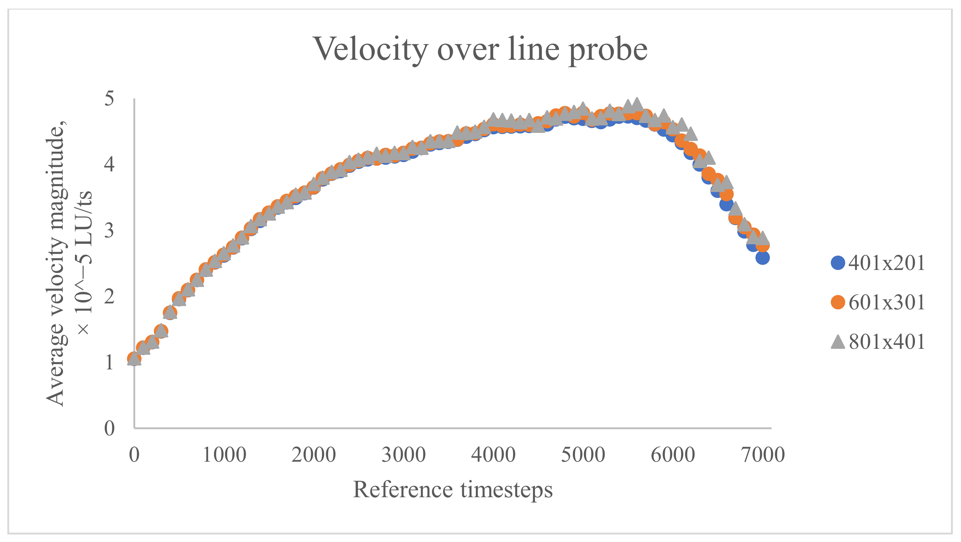
| Grid Size, LU2 | CO2 Flux, × 10−7 LU/ts | Relative Error (%) |
|---|---|---|
| 401 × 201 | 3.590 | - |
| 601 × 301 | 3.651 | 1.7% |
| 801 × 401 | 3.679 | 0.76% |
Publisher’s Note: MDPI stays neutral with regard to jurisdictional claims in published maps and institutional affiliations. |
© 2021 by the authors. Licensee MDPI, Basel, Switzerland. This article is an open access article distributed under the terms and conditions of the Creative Commons Attribution (CC BY) license (https://creativecommons.org/licenses/by/4.0/).
Share and Cite
Ashirbekov, A.; Kabdenova, B.; Monaco, E.; Rojas-Solórzano, L.R. Equation of State’s Crossover Enhancement of Pseudopotential Lattice Boltzmann Modeling of CO2 Flow in Homogeneous Porous Media. Fluids 2021, 6, 434. https://doi.org/10.3390/fluids6120434
Ashirbekov A, Kabdenova B, Monaco E, Rojas-Solórzano LR. Equation of State’s Crossover Enhancement of Pseudopotential Lattice Boltzmann Modeling of CO2 Flow in Homogeneous Porous Media. Fluids. 2021; 6(12):434. https://doi.org/10.3390/fluids6120434
Chicago/Turabian StyleAshirbekov, Assetbek, Bagdagul Kabdenova, Ernesto Monaco, and Luis R. Rojas-Solórzano. 2021. "Equation of State’s Crossover Enhancement of Pseudopotential Lattice Boltzmann Modeling of CO2 Flow in Homogeneous Porous Media" Fluids 6, no. 12: 434. https://doi.org/10.3390/fluids6120434