The Finite Size Lyapunov Exponent and the Finite Amplitude Growth Rate

Abstract

The finite size Lyapunov exponent (FSLE) has been used extensively since the late 1990s to diagnose turbulent regimes from Lagrangian experiments and to detect Lagrangian coherent structures in geophysical flows and two-dimensional turbulence. Historically, the FSLE was defined in terms of its computational method rather than via a mathematical formulation, and the behavior of the FSLE in the turbulent inertial ranges is based primarily on scaling arguments. Here, we propose an exact definition of the FSLE based on conditional averaging of the finite amplitude growth rate (FAGR) of the particle pair separation. With this new definition, we show that the FSLE is a close proxy for the inverse structural time, a concept introduced a decade before the FSLE. The (in)dependence of the FSLE on initial conditions is also discussed, as well as the links between the FAGR and other relevant Lagrangian metrics, such as the finite time Lyapunov exponent and the second-order velocity structure function.

1. Introduction

Lagrangian relative dispersion experiments, consisting in the simultaneous release of large numbers of particle pairs and studying their separation characteristics, are a powerful way to assess turbulent properties of a flow. Various metrics have been used to study pair dispersion. An example is the “relative dispersion”, which derives from averaging squared pair separations at fixed times. Similar such time-based metrics include the relative diffusivity and the separation kurtosis (e.g., [1,2,3]).

It was recognized though that such averaging could potentially smear out dependences if the dispersive properties vary with scale. Thus, separation-based averages were introduced. Among the most well-known of these is the finite size Lyapunov exponent (FSLE), first introduced by Aurell et al. [4] and Artale et al. [5] as a measure of the chaoticity in turbulent flows. The FSLE has been used extensively subsequently [3,6,7,8,9,10,11,12,13].

Aurell et al. [4] defined the FSLE as the ensemble-averaged inverse time $T^{-1}$ necessary for a given perturbation $\delta v$ to grow by a given factor $\alpha$, multiplied by the natural logarithm of this factor:

$$\begin{array}{c}\hfill \lambda \left(\delta v\right)=〈\frac{1}{T\left(\delta v\right)}〉ln\left(\alpha \right),\end{array}$$

(1)

In the limit of small perturbations, the FSLE recovers the finite time Lyapunov exponent.

Our subsequent focus is on particles in turbulent flows, so we take $\delta v$ to be the distance between two particles $r=|{\mathbf{x}}_{\mathbf{2}}-{\mathbf{x}}_{\mathbf{1}}|$, where ${\mathbf{x}}_{\mathbf{2}}$ and ${\mathbf{x}}_{\mathbf{1}}$ are the individual positions of the particles. Defining a series of geometrically-increasing reference separations $r_i$ ($i\in [1,N]$), with $\alpha =\frac{r_{i+1}}{r_i}$, the FSLE is:

$$\begin{array}{c}\hfill {\lambda }_i=ln\left(\alpha \right)〈\frac{1}{T_i}〉\end{array}$$

(2)

where $T_i$ is the time for the separation to grow from $r_i$ to $\alpha r_i$ (also referred to as the “exit time” [14]). Note that for finite amplitude perturbations, the FSLE depends on the chosen norm [15]. In this work, we chose the Euclidian norm of the separation vector, the most common norm used in two-dimensional and geophysical turbulence.

The FSLE has been used frequently to analyze in situ data [6,7,8]). In a number of studies, an alternate expression was used, in which the ensemble-average of the inverse exit time is replaced by the inverse ensemble-average of the exit time [3,5,9,10,12,13,16]. It should be emphasized that the inverse of the ensemble-average $\frac{1}{\langle T\rangle }$ and the ensemble-average of the inverse $\langle \frac{1}{T}\rangle$ are generally not equal. Hereafter, we employ the original definition Equation (2). As shown below, this is advantageously related to the separation growth rate, so that an analytical expression of the FSLE becomes possible.

Cencini and Vulpiani [15] lamented the lack of mathematical rigor in the definition of FSLE, which is based on a computational procedure. As such, we lack analytical expressions for the FSLE, except under exponential pair dispersion. The method also involves several arguably arbitrary computational choices. Pair separations generally do not increase monotonically in time, so one must decide which “crossing time” to use for the bins: that of the first crossing, the fastest crossing or a mean of all crossing times. The choice can affect the results. Using the fastest crossing for example biases the measure to periods of rapid growth.

There are also technical issues with the FSLE. If the pair separation velocity exceeds $(\alpha -1)r_i/\delta t$ (where $\delta t$ is the sampling rate), the separation will cross two successive thresholds in one time step [3,9,17]. If a minimum time is used, the FSLE can saturate, yielding the false impression of exponential growth [3,8,17]. This issue is usually avoided by increasing the separation factor, $\alpha$, or by interpolating the pair separations to smaller time steps [3,9]. Such interpolation can alter the slope of FSLE and hence the inferred growth law.

Furthermore, by recording only times for increasing growth one neglects converging pairs. Thus, only positive FSLEs are obtained. With synthetic trajectories, obtained from modelled velocity fields, this can be addressed by integrating trajectories forward and backward in time, yielding positive and negative FSLEs, respectively. This is commonly done to detect Lagrangian coherent structures, where repelling (attracting) structures are associated with positive (negative) FSLEs [18,19,20]. However, such backward integrations are of course not possible with in situ data.

Following Letz and Kantz [21], Cencini and Vulpiani [15] proposed an alternate scale-dependent growth indicator:

$$\begin{array}{}\mathrm{(3)}& \hfill \tilde{\lambda }\left(r_i\right)& =& \frac{1}{2\langle r^2\left(t\right)\rangle }\frac{d\langle r^2\left(t\right)\rangle }{dt}{|}_{\langle r^2\rangle =r_i^2},\hfill \mathrm{(4)}& & =& \frac{d}{dt}〈ln\left(r\left(t\right)\right)〉{|}_{\langle ln\left(r\right)\rangle =ln\left(r_i\right)}\hfill \end{array}$$

This measure can be positive or negative. However, the latter authors dismissed $\tilde{\lambda }\left(r_i\right)$ as a proper proxy for FSLE because it is not strictly a separation-based metric, as the relative dispersion involves averaging in time. Such averaging potentially combines contributions from different dispersive regimes. The authors also noted that $\tilde{\lambda }\left(r_i\right)$ is potentially sensitive to the initial conditions.

Hereafter, we propose a rigorous derivation of $\tilde{\lambda }$ (that we refer to as the Cencini–Vulpiani exponent; CVE) by introducing a new variable: the single-realization finite amplitude growth rate, $\gamma$ (FAGR). The derivation advantageously reveals the links to other dispersion metrics, such as the Finite time Lyapunov exponent, the relative diffusivity and velocity structure functions. We show too that the CVE can be an exact proxy for FSLE, under the appropriate conditional averaging. Thus, it is possible to build a mathematical definition of the FSLE using the CVE.

2. Numerical Experiment

We will test the various metrics using three 2D simulations described in [22]. The code solves the 2D vorticity equation:

$$\frac{\partial \zeta }{\partial t}+J(\psi ,\zeta )=\mathcal{F}-r\zeta$$

(5)

where $\psi$ is the streamfunction, $\zeta ={\nabla }^2\psi$ the relative vorticity and $J(a,b)$ the Jacobian function. The forcing, $\mathcal{F}$, is applied with random phases in an isotropic wavenumber band, which is varied. Rayleigh dissipation is used, with a constant (Ekman) coefficient of $r=0.1$. Small-scale variance is removed via an exponential cut-off filter [23]. The forcing amplitude was adjusted so that the equilibrated kinetic energy was 1.0. The domain is doubly periodic, with $512\times 512$ grid points.

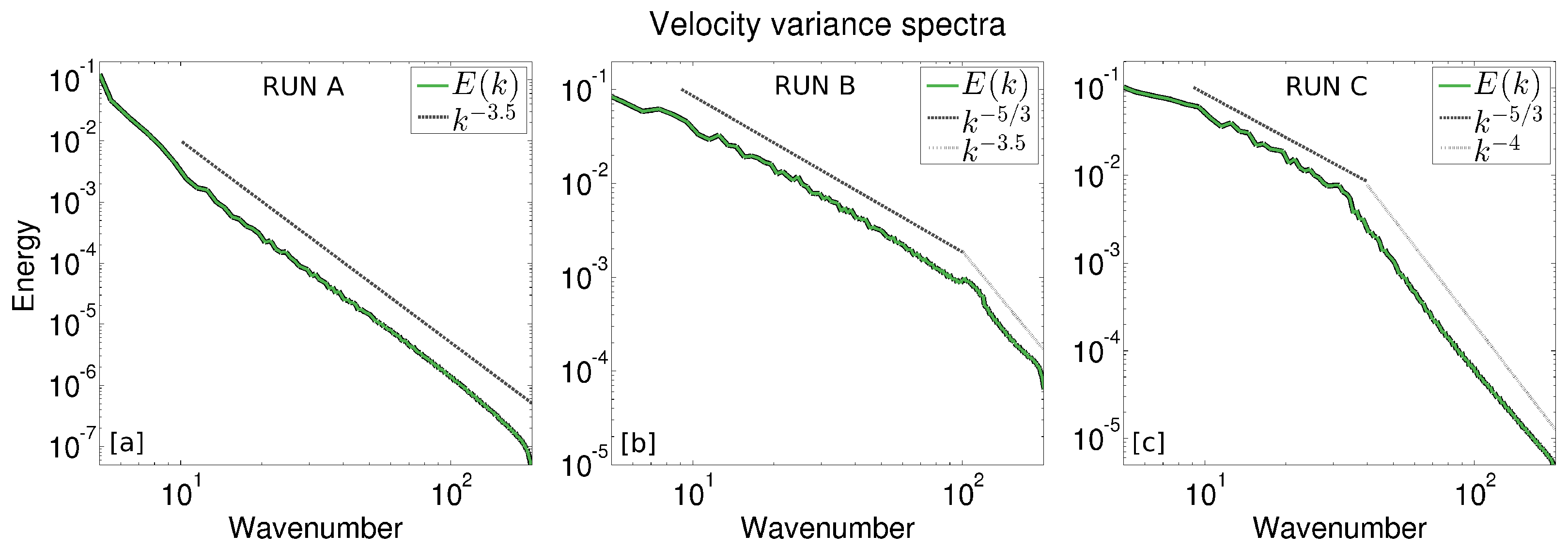
We will focus on three simulations hereafter. The velocity variance spectra for these are shown in Figure 1. In run A (panel a), the forced wavenumber range lies between k = [1, 5], yielding an enstrophy inertial range (non-local dispersion) approximately between k = [10, 100]. The spectral slope is somewhat steeper than the expected $k^{-3}$ [24] due to the dissipation. In run B (panel b), the forced wave numbers range between k = [100, 120], yielding an energy inertial range (local dispersion) with a $k^{-5/3}$ spectrum in the range k = [10, 100]. In run C, the forcing is applied at intermediate wavenumbers (k = [30, 35]). An energy cascade occurs at smaller wavenumbers, again with a $k^{-5/3}$ spectrum. The spectral slope at high wavenumbers in this case is at ≈$k^{-4}$, again due to the imposed dissipation. However, such a slope will produce exponential (non-local) dispersion nevertheless [25].

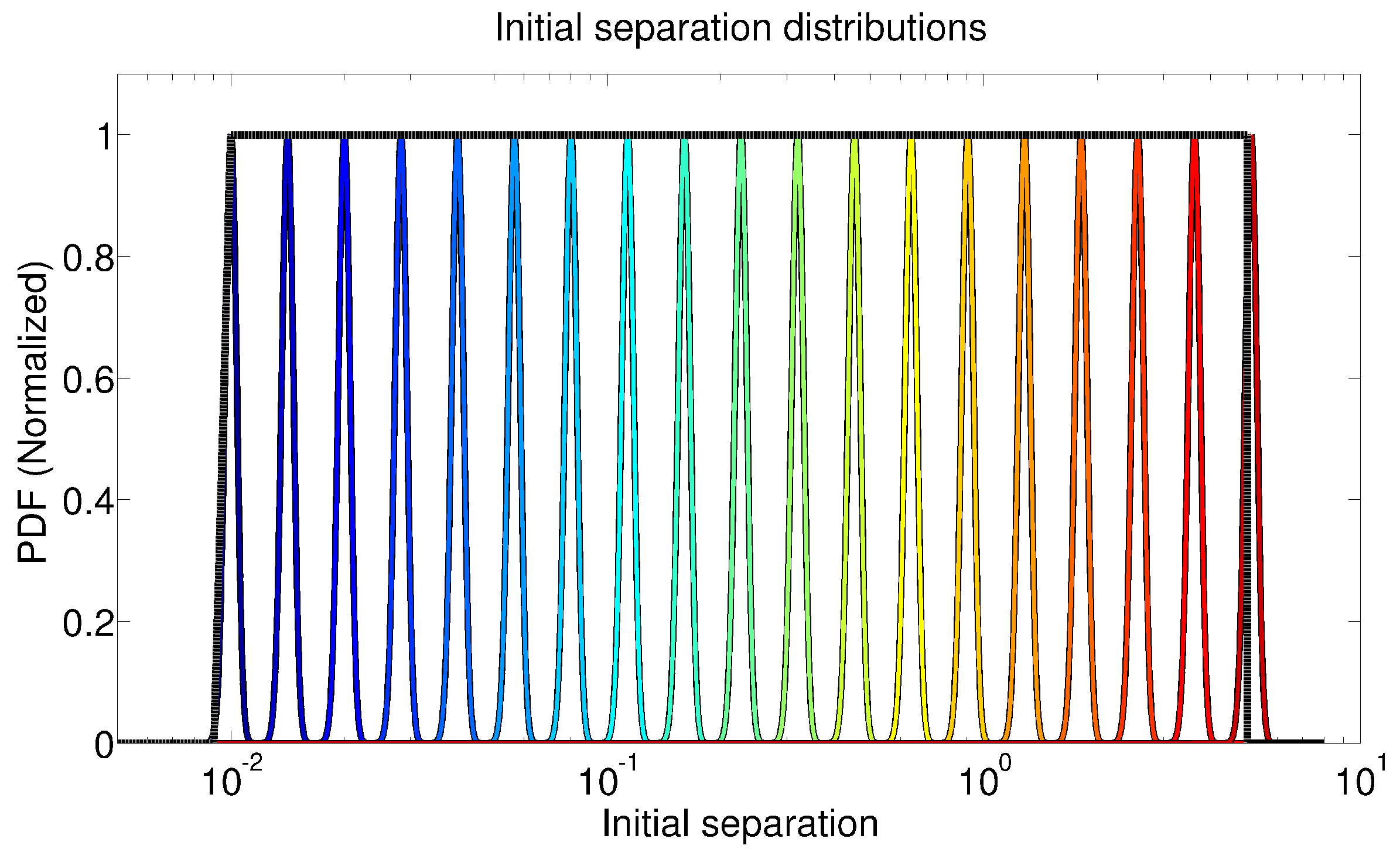
Particles were deployed after the kinetic energy had equilibrated, and trajectories were “unwrapped” as particles exited the original domain, allowing separations to exceed the domain scale $2\pi \times 2\pi$. The particles were deployed on square grids with a spacing $\delta x=0.01$. Initial separations ranged between ${10}^{-2}$ and approximately 5, and each interval of $0.01$ contains 1000 pairs.

In some cases, the FSLE and CVE are computed using a selected single initial separation (e.g., $r=0.01$). Then the initial pair separation has a Dirac distribution (e.g., [26,27]). However, a well-known advantage of FSLE over other Lagrangian metrics is its insensitivity to initial conditions, allowing the use of all available pairs regardless of their initial separation [3]. This permits larger numbers of pairs and hence improved statistics. Thus, we also considered the case with a flat (Heaviside) distribution, with separations ranging from 0.01 to 5. When unspecified hereafter, the initial conditions correspond to this flat distribution. A schematic view of the initial separation distributions used in this study is shown in Figure 2.

3. The Finite Amplitude Growth Rate

3.1. Definition

Since the pair separation $r\left(t\right)$ is positive definite and a continuous function of time, there exists a time-dependent function $\gamma \left(t\right)$ such that the value of r at time $t+\delta t$ is related to the value of r at time t following:

$$\begin{array}{ccc}\hfill r(t+\delta t)& =& r\left(t\right)e^{\gamma \left(t\right)\delta t}.\hfill \end{array}$$

(6)

Hereafter, we refer to the function $\gamma \left(t\right)$ as the single-realization finite amplitude growth rate (FAGR). From Equation (6), we may express $\gamma \left(t\right)$ as a function of separation and time:

$$\begin{array}{}\mathrm{(7)}& \hfill \gamma \left(t\right)& =& \frac{1}{\delta t}ln\left(\frac{r(t+\delta t)}{r\left(t\right)}\right)\hfill \mathrm{(8)}& & =& \frac{ln\left[r\right(t+\delta t\left)\right]-ln\left[r\right(t\left)\right]}{\delta t}.\hfill \end{array}$$

In the small time step asymptotic limit, $ln\left[r\right(t\left)\right]$ is continuous and differentiable. Thus, we have:

$$\begin{array}{c}\hfill \underset{\delta t\to 0}{lim}\gamma \left(t\right)=\frac{d}{dt}ln\left[r\left(t\right)\right],\end{array}$$

(9)

or equivalently:

$$\begin{array}{c}\hfill \gamma \left(t\right)=\frac{1}{r\left(t\right)}\frac{dr\left(t\right)}{dt}.\end{array}$$

(10)

When ensemble-averaged over all pairs at constant separation $r_i$, the FAGR $\gamma \left(t\right)$ recovers the CVE $\tilde{\lambda }\left(t\right)$.

3.2. Properties

Through appropriate averaging and/or integration, it is possible to express a number of meaningful Lagrangian metrics in terms of $\gamma$.

For example, the finite time Lyapunov exponent (FTLE), ${\lambda }_T$, is defined for an initial separation $r\left(0\right)={\delta }_0$ as:

$$\begin{array}{ccc}\hfill {\lambda }_T\left(t\right)& =& \underset{{\delta }_0\to 0}{lim}\frac{1}{t}ln\left(\frac{r\left(t\right)}{{\delta }_0}\right).\hfill \end{array}$$

(11)

e.g., [28,29,30]. Integrating Equation (10) from 0 to time t, we get:

$$\begin{array}{ccc}\hfill {\int }_0^t\gamma \left(\tau \right)d\tau & =& ln\left(\frac{r\left(t\right)}{{\delta }_0}\right)\hfill \end{array}$$

(12)

Dividing both sides by time, t, the FTLE is seen to be the time-average value of the FAGR from the initial time to time t for infinitesimal initial separation:

$$\begin{array}{ccc}\hfill {\lambda }_T& =& \underset{{\delta }_0\to 0}{lim}{〈\gamma 〉}_0^t,\hfill \end{array}$$

(13)

$$\begin{array}{ccc}\hfill {\langle ·\rangle }_0^t& \equiv & \frac{1}{t}{\int }_0^t·d\tau \hfill \end{array}$$

(14)

The second-order velocity structure function, the ensemble-average squared separation velocity at constant separation, can also be expressed in terms of $\gamma$. From Equation (10), the separation velocity, $u=\frac{dr}{dt}$, can be written:

$$\begin{array}{ccc}\hfill u\left(t\right)& =& \gamma \left(t\right)r\left(t\right).\hfill \end{array}$$

(15)

Ensemble averaging the squared velocity at a given separation yields:

$$\begin{array}{ccc}\hfill S_2\left(r\right)& =& {〈u^2〉}_r=r^2{〈{\gamma }^2〉}_r,\hfill \end{array}$$

(16)

where ${\langle ·\rangle }_r$ denotes averaging at constant separation. The simple relationship between $\gamma$ and $S_2$ is convenient, as $S_2$ is related to the Eulerian energy spectrum via the Hankel transform [22].

The relative diffusivity can also be written in terms of $\gamma$. Although a scale-dependent function, similar to the velocity structure functions, it is computed by averaging at constant time rather than separation:

$$\begin{array}{ccc}\hfill K\left(t\right)& =& \frac{1}{2}{〈\frac{d{r}^2}{dt}〉}_t.\hfill \end{array}$$

(17)

From Equation (10), we have:

$$K\left(t\right)={〈\gamma \left(t\right)r^2\left(t\right)〉}_t$$

(18)

Using Equations (12) and (14), we can express the diffusivity in terms of the initial separation, ${\delta }_0$, the FAGR and the FTLE, ${\lambda }_T$:

$$\begin{array}{ccc}\hfill K\left(t\right)& =& {〈{\delta }_0^2\gamma \left(t\right)e^{2t{\lambda }_T\left(t\right)}〉}_t.\hfill \end{array}$$

(19)

If the initial separation ${\delta }_0$ is continuously distributed with a probability density function, $p\left({\delta }_0\right)$, we have:

$$\begin{array}{ccc}\hfill K\left(t\right)& =& {\int }_{{\delta }_{min}}^{{\delta }_{max}}{〈\gamma e^{2t{\lambda }_T}〉}_{({\delta }_0,t)}{\delta }_0^{2}p\left({\delta }_0\right)d{\delta }_0.\hfill \end{array}$$

(20)

Here, the averaging is performed on pairs with an initial separation ${\delta }_0$ at a fixed time. If all pairs have the same initial separation (Dirac distribution), we have:

$$\begin{array}{ccc}\hfill K\left(t\right)& =& {\delta }_0^2{〈\gamma e^{2t{\lambda }_T}〉}_t,\hfill \end{array}$$

(21)

where ${〈·〉}_t$ represents averaging all pairs at a given time t.

One can furthermore use $\gamma$ to express Babiano et al. [31]’s instantaneous relative dispersion coefficient, a time-independent proxy for the relative diffusivity:

$$\begin{array}{ccc}\hfill X\left(r\right)& =& {〈{\left(\frac{1}{2}\frac{d}{dt}{r}^2\right)}^2〉}_r^{1/2},\hfill \\ & =& r^2{〈{\gamma }^2〉}_r^{1/2},\hfill \end{array}$$

(22)

where ${〈·〉}_r$ represent averaging pairs with constant separation r.

4. Finite Size Lyapunov Exponents

To express the FSLE $\lambda$ in terms of the FAGR, $\gamma$, we use a similar procedure as for the FTLE, integrating Equation (10) from time t to a later time $t+T$, yielding:

$$\begin{array}{ccc}\hfill {\int }_t^{t+T}\gamma \left(\tau \right)d\tau & =& ln\left(\frac{r(t+T)}{r\left(t\right)}\right).\hfill \end{array}$$

(23)

Introducing the time average operator ${〈·〉}_t^{t+T}=\frac{1}{T}{\int }_t^{t+T}·d\tau$, we have:

$$\begin{array}{ccc}\hfill r(t+T)& =& r\left(t\right)exp\left\{T{〈\gamma 〉}_t^{t+T}\right\}\hfill \end{array}$$

(24)

Now assume that $T_i$ is the time required for the separation to grow from a reference separation $r_i$ to another separation $r_{i+1}$. Averaging between time t and $t+T_i$ is then equivalent to averaging between separations $r_i$ and $r_{i+1}$. Then for each particle pair:

$$\begin{array}{ccc}\hfill \frac{ln(r_{i+1}/r_i)}{T_i}& =& {〈\gamma 〉}_{r_i}^{r_{i+1}}.\hfill \end{array}$$

(25)

The reference separations are assumed to increase geometrically, i.e., $r_{i+1}=\alpha r_i$. By ensemble averaging Equation (25) over all pairs, we may define the variable $\widehat{\lambda }(r_i,\alpha )$:

$$\begin{array}{ccc}\hfill \widehat{\lambda }(r_i,\alpha )& =& 〈{〈\gamma 〉}_{r_i}^{\alpha r_i}〉=〈\frac{1}{T_i}〉ln\left(\alpha \right)\hfill \end{array}$$

(26)

Then, noting that $\frac{1}{r}\frac{dr}{dt}=\frac{1}{2r^2}\frac{d{r}^2}{dt}$, one finds that $\widehat{\lambda }$ is exactly equal to the CVE $\tilde{\lambda }$:

$$\begin{array}{}\mathrm{(27)}& \hfill 〈{〈\gamma 〉}_{r_i}^{\alpha r_i}〉& =& {〈\gamma 〉}_{r_i}\hfill \mathrm{(28)}& & =& \frac{1}{2r_i^2}\frac{d}{dt}{\langle r^2\rangle }_{r_i},\hfill \mathrm{(29)}& & =& \tilde{\lambda }\left(r_i\right)\hfill \end{array}$$

where ${〈·〉}_{r_i}$ is the ensemble average over all pairs at separation $r_i$.

The only difference between CVE and FSLE then lies in the ensemble averaging. The FSLE assumes pair separations grow between adjacent reference separations, thereby neglecting decaying pair separations. In Equation (26), the averaging is performed over all separations between the two thresholds, both growing and decaying. Thus, we can recover the FSLE from $\widehat{\lambda }$ by averaging only positive values of ${\langle \gamma \rangle }_{r_i}^{r_{i+1}}$:

$$\begin{array}{ccc}\hfill {\lambda }_i& =& {〈{〈\gamma 〉}_{r_i}^{r_{i+1}}〉}_{{\langle \gamma \rangle }_{r_i}^{r_{i+1}}>0}\hfill \end{array}$$

(30)

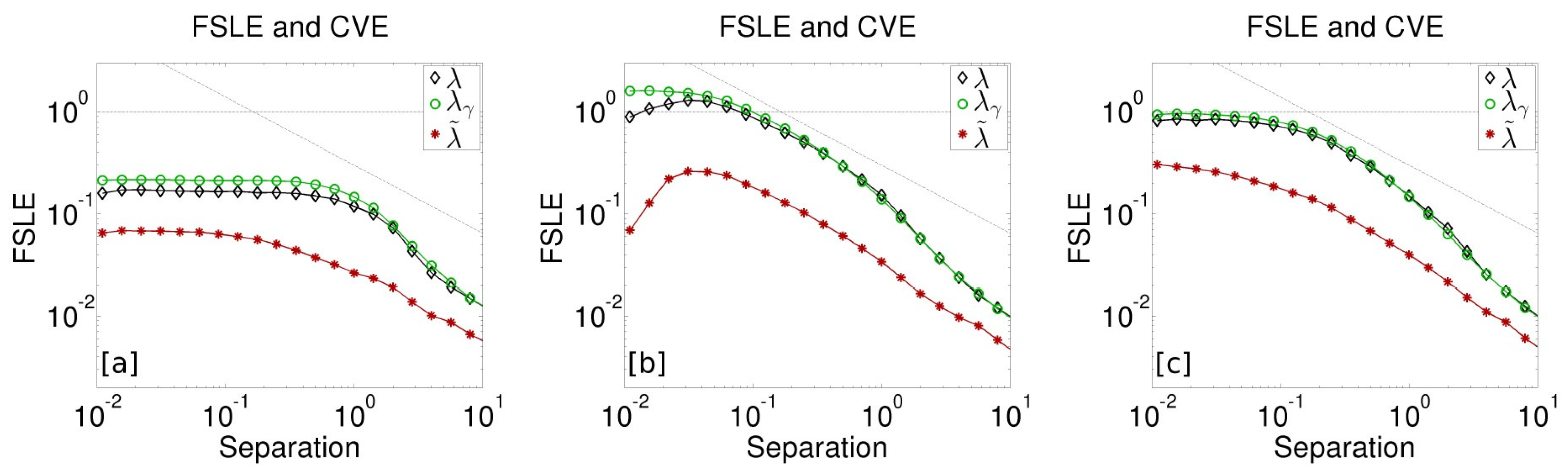
The FSLE computed from Equation (30) (${\lambda }_{\gamma }$, green circles) and the FSLE computed from the pair separations using the first crossing criterion ($\lambda$, black diamonds) are compared in Figure 3 for the three model runs. The two agree well, exhibiting the same patterns and slopes over the same separations. The plateau at small separations, indicating exponential growth, is clear with both methods. The values of ${\lambda }_{\gamma }$ are somewhat larger, due to the aforementioned time step bias of the first crossing procedure (the FSLE from Equation (30) is not subject to this). In contrast, the CVE, $\tilde{\lambda }$, is nearly one order of magnitude smaller at all scales. It also lacks clearly distinct power law slopes, and the exponential growth range is less obvious. This supports Cencini and Vulpiani [15]’s statement that the CVE (where averaging is performed on all pairs) cannot be used as a proxy for FSLE (where averaging is only performed on separating pairs).

In the limit of small bin widths, Equation (30) can be expressed as:

$$\begin{array}{c}\hfill li{m}_{\alpha \to 1}\lambda \left(r\right)={〈\gamma 〉}_{(r,\gamma >0)},\end{array}$$

(31)

where ${〈\gamma 〉}_{(r,\gamma >0)}$ represents averaging positive values of $\gamma$ at constant separation. Defining a positive scale-averaged equivalent to the relative diffusivity:

$$\begin{array}{}\mathrm{(32)}& \hfill K_s\left(r\right)& =& \frac{1}{2}{〈\frac{d{r}^2}{dt}〉}_{(r,\frac{d{r}^2}{dt}>0)}\hfill \mathrm{(33)}& & =& \frac{1}{r^2}〈\gamma 〉{}_{(r,\gamma >0)}\hfill \end{array}$$

we obtain an alternative definition of FSLE:

$$\begin{array}{ccc}\hfill \lambda \left(r\right)& =& \frac{K_s\left(r\right)}{r^2}.\hfill \end{array}$$

(34)

This closely resembles the inverse of Babiano et al. [31]’s “structural time”, $\tau$, which derives from the instantaneous dispersion coefficient in Equation (22):

$$\begin{array}{ccc}\hfill \tau \left(r\right)& =& \frac{r^2}{X\left(r\right)}.\hfill \end{array}$$

(35)

We refer hereafter to the reciprocal of this, ${\lambda }_B\equiv {\tau }^{-1}$, as the inverse structural time (IST).

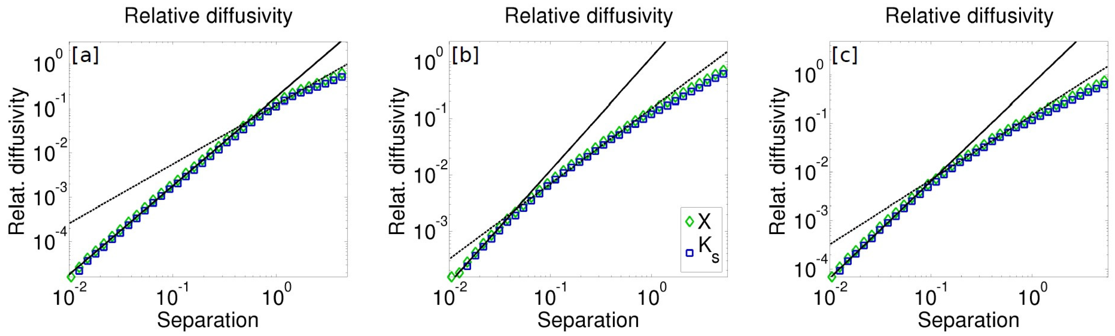
Comparisons between the scale-averaged positive relative diffusivity $K_s\left(r\right)$ and the instantaneous dispersion coefficient $X\left(r\right)$ are shown in Figure 4. For all three runs, $K_s\left(r\right)$ and $X\left(r\right)$ exhibit a strikingly similar behaviour at all scales. Although the three runs exhibit different regimes, the ratio $X/K_s$ (not shown) is approximately constant, with mean values of 1.25, 1.22, and 1.23 for runs A, B, and C, respectively. The similarity between $K_s\left(r\right)$ and $X\left(r\right)$ is not trivial. At a given reference separation, $X\left(r\right)$ is the root mean square of the single-realization relative diffusivity $\frac{1}{2}\frac{d{r}^2}{dt}$, using the entire distribution in the averaging (including negative values), while $K_s\left(r\right)$ only uses positive values. While the link between $K_s\left(r\right)$ and $X\left(r\right)$ is an interesting topic, it is beyond the scope of the present paper and will remain to be investigated.

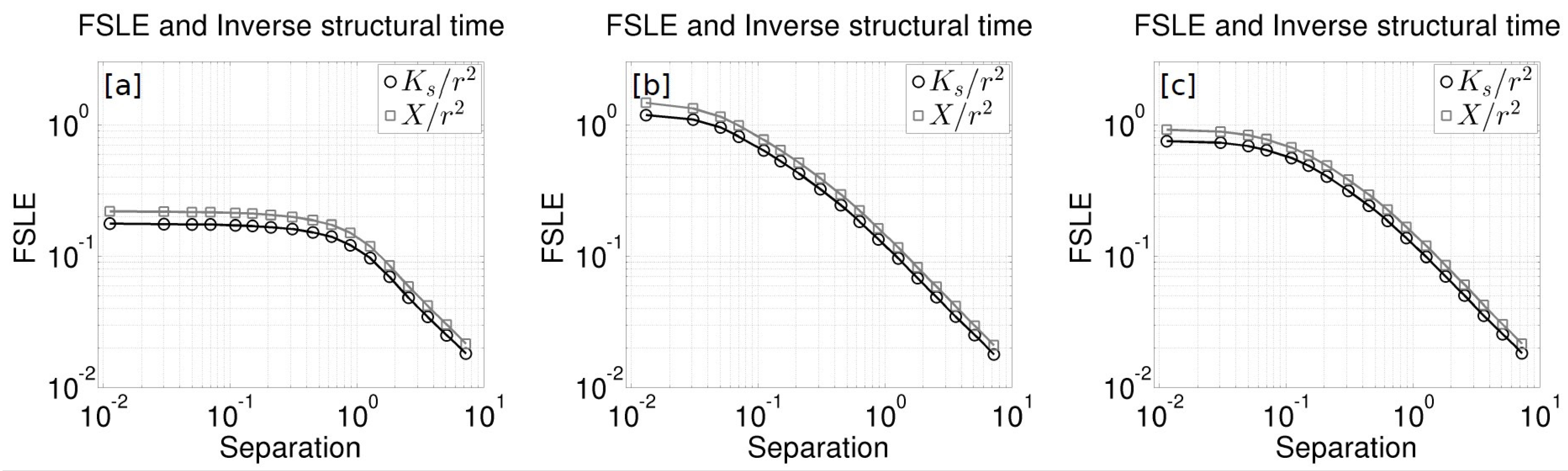
Figure 5 compares the FSLE computed in the asymptotic limit (Equation (34)) and the IST. As expected from the agreement between $X\left(r\right)$ and $K_s\left(r\right)$, the close similarity of the curves confirms that FSLE in the small $\alpha$ limit is a proxy for the IST. While the lack of an analytical link between $X\left(r\right)$ and $K_s\left(r\right)$ in the present work prevents definitive conclusions, this result is appealing and holds for 3 simulations with different turbulent regimes, including finite inertial ranges.

The instantaneous dispersion coefficient $X\left(r\right)$ is directly linked to the longitudinal second-order velocity structure function $S_{2l}\left(r\right)$ [2]:

$$\begin{array}{ccc}\hfill X\left(r\right)& =& r\sqrt{S_{2l}\left(r\right)},\hfill \end{array}$$

(36)

so the IST can also be expressed in terms of $S_{2l}\left(r\right)$:

$$\begin{array}{ccc}\hfill {\lambda }_B\left(r\right)& =& r\sqrt{S_{2l}\left(r\right)},\hfill \end{array}$$

(37)

In turn, LaCasce [22] showed that the Eulerian velocity variance spectrum was linked with the longitudinal second-order velocity structure function via the inverse Hankel transform:

$$\begin{array}{ccc}\hfill E\left(K\right)& =& \frac{1}{2}{\int }_0^{\infty }\left[E_t-\frac{S_{2l}\left(r\right)}{2}\right]K^2{r}^2{J}_1\left(Kr\right)dr,\hfill \end{array}$$

(38)

where $E_t$ is the total kinetic energy, K is the wavenumber, and $J_1$ is the first-order Bessel function. Hence, the Eulerian velocity variance spectrum and the IST ${\lambda }_B$ are linked:

$$\begin{array}{ccc}\hfill E\left(K\right)& =& \frac{1}{2}{\int }_0^{\infty }\left[E_t-\frac{{\lambda }_B^2\left(r\right)r^2}{2}\right]K^2{r}^2{J}_1\left(Kr\right)dr,\hfill \end{array}$$

(39)

Thus, if confirmed in further analytical, experimental and numerical studies, the equivalence between FSLE and IST would yield intersting properties for FSLE, with a direct link to the Eulerian velocity variance spectrum.

5. Dependence on Initial Conditions

Cencini and Vulpiani [15] argued that the major difference between the CVE and the FSLE is that the former depends on initial conditions while the latter does not. To explore this, we computed the CVE and FSLE for different initial separations. In each case, all pairs have the same initial separation (the initial separation PDF is a delta function). We then vary the separation from the smallest to the largest reference separation threshold $r_i$, as in Figure 2.

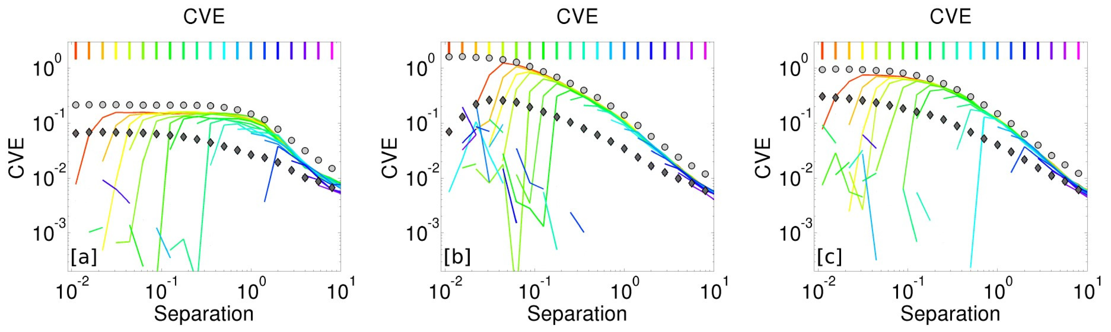
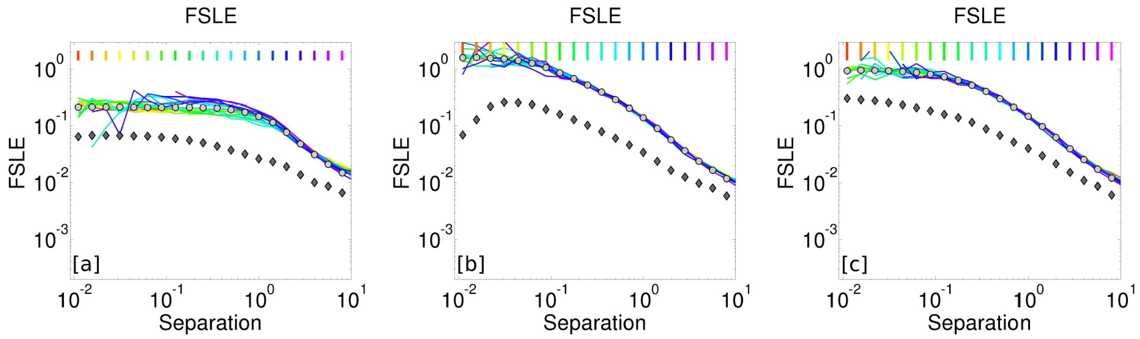
The results are compared to the reference calculation (which uses all available pairs, i.e., Heaviside-distributed initial separations) in Figure 6 and Figure 7 for the CVE and FSLE, respectively. For all three runs, the CVE converges to the reference FSLE for separations larger than the initial separation, as pairs are on average separating at these scales. The values for smaller scales are more variable, as pairs must first converge. Thus, the smaller scales have more negative values on average. In contrast, the FSLE converges to the reference FSLE at all scales.

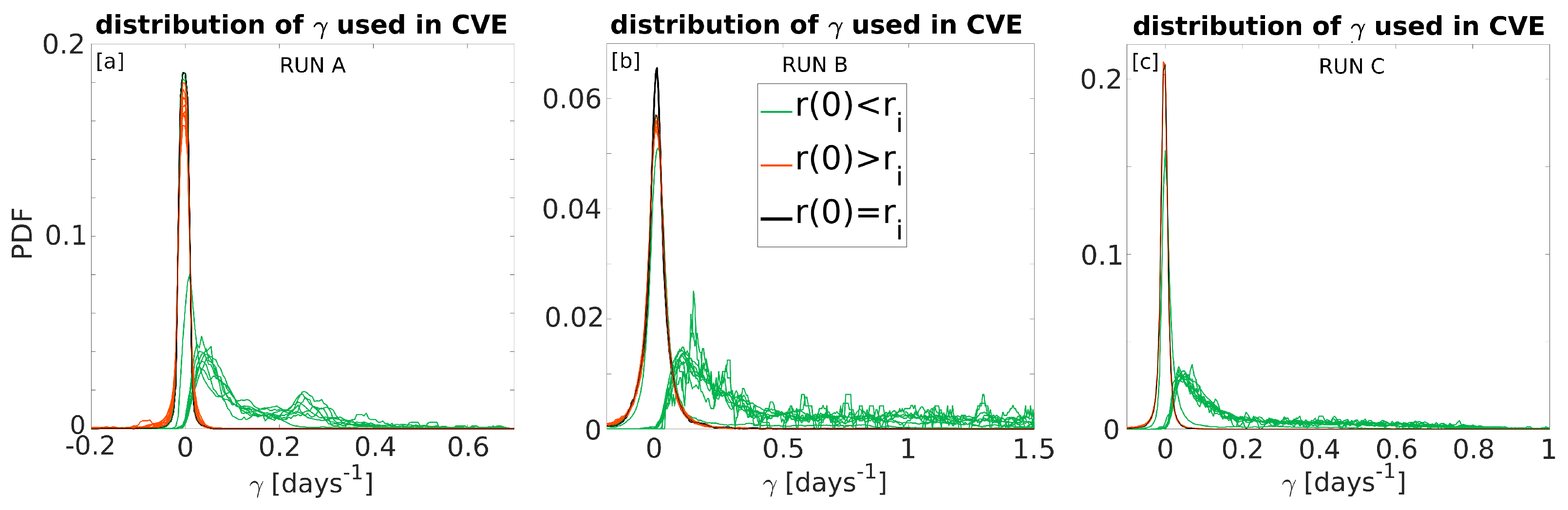
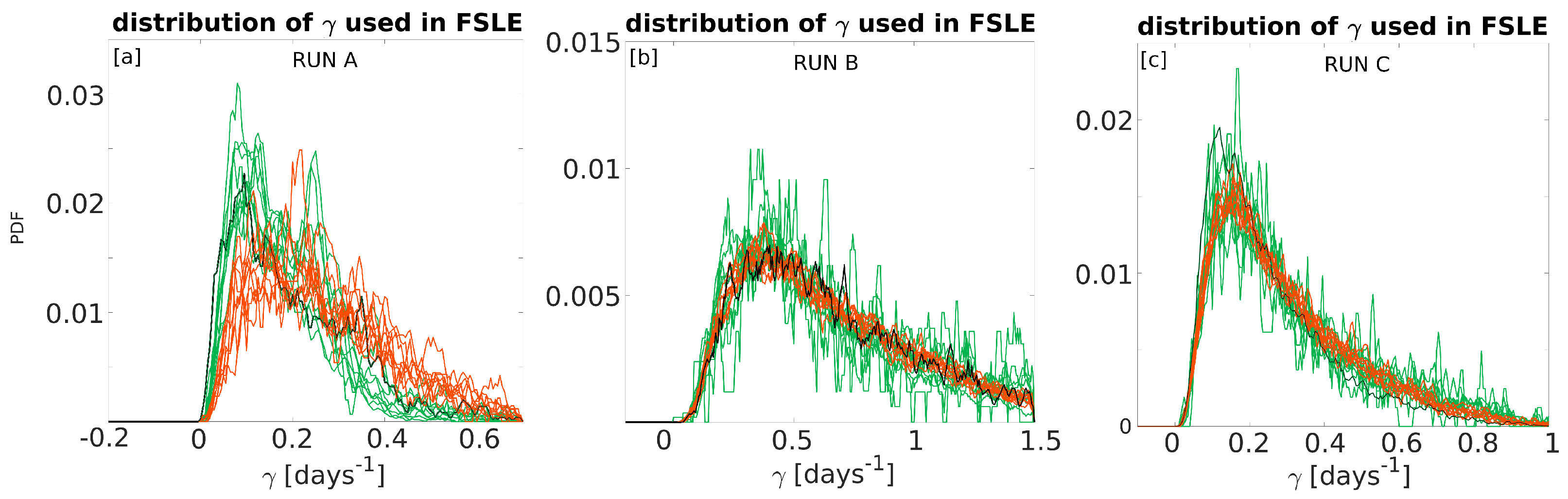
We then compare the distribution of $\gamma$ values used in the averages for a given reference separation threshold. The results for a reference separation $r_i=0.35$ are shown in Figure 8 and Figure 9, for the CVE and FSLE, respectively. In the case of the CVE, for initial separations larger than the reference separation, $\gamma$ has a Gaussian distribution centered at 0, showing that growing and decaying separations are equally likely. For initial separations smaller than the reference separation, the distributions are skewed towards positive $\gamma$. In contrast, the distribution of $\gamma$ used in the FSLE computation is not sensitive to the initial separation, with similar PDFs obtained for all initial conditions.

Thus, the difference between the CVE and FSLE is the conditional averaging over positive values of the FAGR with the FSLE. The ensemble of all pairs whose separation cross the interval $[r_i,r_{i+1}]$ can be decomposed into two sub-ensembles of pairs with an initial separation of $r_i$ or $r_{i+1}$. If we write ${\gamma }_i$ and ${\gamma }_{i+1}$ to identify the FAGR of these sub-ensembles, the ensemble averaging of Equation (25) can be written:

$$\begin{array}{ccc}\hfill 〈\gamma 〉& =& \frac{N_i}{N}〈{\gamma }_i〉+\frac{N_{i+1}}{N}〈{\gamma }_{i+1}〉\hfill \end{array}$$

(40)

Thus, $\langle \gamma \rangle$ is a weighted average of positive and negative FAGRs: pairs with initial separation $r_i$ can only enter the interval if ${\gamma }_i$ is positive, and oppositely for ${\gamma }_{i+1}$. Hence, the CVE is the weighted average of the positive and negative FSLEs and transforming the CVE to the standard FSLE is equivalent to suppressing the last term of (40).

6. Concluding Remarks

By introducing the FAGR, based on the separation of individual pairs, we have derived an alternative mathematical definition of the FSLE. The FAGR can also be used to derive other common dispersion metrics, like the FTLE and the second-order structure function. With vanishing bin sizes, the new FSLE is also a close proxy to the IST; both are linked to a form of the separation-averaged relative diffusivity (the instantaneous dispersion coefficient $X\left(r\right)$ for the IST, and the separation-averaged positive diffusivity $K_s\left(r\right)$ for the FSLE). Interestingly, while Babiano et al. [31]’s structural time has not been adopted to the same degree as the FSLE in relative dispersion studies, it is an equivalent concept, and was introduced over a decade earlier. Further, the IST was shown to be linked to the Eulerian velocity variance spectrum through an exact relationship; in contrast, the relationship between FSLE and the Eulerian velocity variance spectrum is based on scaling arguments. It might thus be relevant to favor the use of the IST over the FSLE to infer turbulent regimes from particle pair statistics, although the present results suggest they are likely equivalent.

The FAGR also elucidates the FSLE’s dependence on initial separations. By conditional averaging over positive values of the FAGR (corresponding to separating pairs), the FSLE effectively reduces the sensitivity to initial condition. The CVE on the other hand, by averaging both positive and negative FAGR, is strongly sensitive.

To conclude, we enumerate some advantages of the alternative FSLE definition proposed here over the traditional computation algorithm.

• Since the method relies on averaging all positive FAGR, it does not require arbitrary choices between the first, fastest, or average crossing times.
• The FAGR suppresses the need for higher frequency interpolation at small separation scales, and short-separation scales are more reliably represented.
• The FAGR can be computed and averaged over any given separation set, and the latter is not required to increase geometrically nor to be regular.
• The negative FSLE can be easily obtained by changing the averaging condition from $\langle \gamma \rangle >0$ to $\langle \gamma \rangle <0$.

The new method could thus bring more computational flexibility and reliability to the FSLE, in particular for short separation scales. Note too that, since for very small initial separation the CVE converges towards FSLE, another definition, more analogous to that of FTLE could also be considered:

$$\begin{array}{ccc}\hfill \lambda \left(r\right)& =& \underset{r\left(0\right)\to 0}{lim}\left\{\frac{1}{\delta t}ln\left(\frac{r(t+\delta t)}{r\left(t\right)}\right)\right\}.\hfill \end{array}$$

(41)

References

1. Morel, P.; Larceveque, M. Relative Dispersion of Constant-Level Balloons in the 200-mb General Circulation. J. Atmos. Sci. 1974, 31, 2189–2196. [Google Scholar] [CrossRef]
2. Babiano, A.; Basdevant, C.; Le Roy, P.; Sadourny, R. Relative dispersion in two-dimensional turbulence. J. Fluid Mech. 1990, 214, 535–557. [Google Scholar] [CrossRef]
3. LaCasce, J.H. Statistics from Lagrangian observations. Prog. Oceanogr. 2008, 77, 1–29. [Google Scholar] [CrossRef]
4. Aurell, E.; Boffetta, G.; Crisanti, A.; Paladin, G.; Vulpiani, A. Growth of Noninfinitesimal Perturbations in Turbulence. Phys. Rev. Lett. 1996, 77, 1262–1265. [Google Scholar] [CrossRef] [PubMed] [Green Version]
5. Artale, V.; Boffetta, G.; Celani, A.; Cencini, M.; Vulpiani, A. Dispersion of passive tracers in closed basins: Beyond the diffusion coefficient. Phys. Fluids 1997, 9, 3162–3171. [Google Scholar] [CrossRef] [Green Version]
6. LaCasce, J.H.; Bower, A. Relative dispersion in the subsurface North Atlantic. J. Mar. Res. 2000, 58, 863–894. [Google Scholar] [CrossRef]
7. LaCasce, J.H.; Ohlmann, C. Relative dispersion at the surface of the Gulf of Mexico. J. Mar. Res. 2003, 61, 285–312. [Google Scholar] [CrossRef]
8. Lumpkin, R.; Elipot, S. Surface drifter pair spreading in the North Atlantic. J. Geophys. Res. (Oceans) 2010, 115, C12017. [Google Scholar] [CrossRef] [Green Version]
9. Haza, A.C.; Özgökmen, T.M.; Griffa, A.; Poje, A.C.; Lelong, M.P. How Does Drifter Position Uncertainty Affect Ocean Dispersion Estimates? J. Atmos. Ocean. Technol. 2014, 31, 2809–2828. [Google Scholar] [CrossRef] [Green Version]
10. Berti, S.; Santos, F.A.D.; Lacorata, G.; Vulpiani, A. Lagrangian Drifter Dispersion in the Southwestern Atlantic Ocean. J. Phys. Oceanogr. 2011, 41, 1659–1672. [Google Scholar] [CrossRef] [Green Version]
11. Choi, J.; Bracco, A.; Barkan, R.; Shchepetkin, A.F.; McWilliams, J.C.; Molemaker, J.M. Submesoscale Dynamics in the Northern Gulf of Mexico. Part III: Lagrangian Implications. J. Phys. Oceanogr. 2017, 47, 2361–2376. [Google Scholar] [CrossRef]
12. Corrado, R.; Lacorata, G.; Palatella, L.; Santoleri, R.; Zambianchi, E. General characteristics of relative dispersion in the ocean. Sci. Rep. 2017, 7, 46291. [Google Scholar] [CrossRef] [Green Version]
13. Zavala Sansón, L.; Pérez-Brunius, P.; Sheinbaum, J. Surface Relative Dispersion in the Southwestern Gulf of Mexico. J. Phys. Oceanogr. 2017, 47, 387–403. [Google Scholar] [CrossRef]
14. Boffetta, G.; Celani, A.; Cencini, M.; Lacorata, G.; Vulpiani, A. Nonasymptotic properties of transport and mixing. Chaos 2000, 10, 50–60. [Google Scholar] [CrossRef] [Green Version]
15. Cencini, M.; Vulpiani, A. Finite size Lyapunov exponent: Review on applications. J. Phys. A Math. Theor. 2013, 46, 254019. [Google Scholar] [CrossRef]
16. Meyerjürgens, J.; Ricker, M.; Schakau, V.; Badewien, T.H.; Stanev, E.V. Relative Dispersion of Surface Drifters in the North Sea: The Effect of Tides on Mesoscale Diffusivity. J. Geophys. Res. (Oceans) 2020, 125, e15925. [Google Scholar] [CrossRef]
17. Haza, A.C.; Poje, A.C.; Özgökmen, T.M.; Martin, P. Relative dispersion from a high-resolution coastal model of the Adriatic Sea. Ocean Model. 2008, 22, 48–65. [Google Scholar] [CrossRef]
18. Koh, T.Y.; Legras, B. Hyperbolic lines and the stratospheric polar vortex. Chaos 2002, 12, 382–394. [Google Scholar] [CrossRef] [PubMed]
19. d’Ovidio, F.; Fernández, V.; Hernández-García, E.; López, C. Mixing structures in the Mediterranean Sea from finite-size Lyapunov exponents. Geophys. Res. Lett. 2004, 31, L17203. [Google Scholar] [CrossRef] [Green Version]
20. Bettencourt, J.H.; López, C.; Hernández-García, E. Characterization of coherent structures in three-dimensional turbulent flows using the finite-size Lyapunov exponent. J. Phys. A Math. Theor. 2013, 46, 254022. [Google Scholar] [CrossRef]
21. Letz, T.; Kantz, H. Characterization of sensitivity to finite perturbations. Phys. Rev. E 2000, 61, 2533–2538. [Google Scholar] [CrossRef]
22. LaCasce, J.H. Estimating Eulerian energy spectra from drifters. Fluids 2016, 1, 33. [Google Scholar] [CrossRef] [Green Version]
23. LaCasce, J.H. Baroclinic Vortices over a Sloping Bottom. Ph.D. Thesis, M.I.T./W.H.O.I., Cambridge, MA, USA, 1996. [Google Scholar]
24. Kraichnan, R.H. Inertial Ranges in Two-Dimensional Turbulence. Phys. Fluids 1967, 10, 1417–1423. [Google Scholar] [CrossRef] [Green Version]
25. Lundgren, T.S. Turbulent pair dispersion and scalar diffusion. J. Fluid Mech. 1981, 111, 27–57. [Google Scholar] [CrossRef]
26. Bennett, A.F. Lagrangian Fluid Dynamics; Cambridge University Press: Cambridge, UK, 2006; p. 286. [Google Scholar]
27. LaCasce, J.H. Relative displacement PDFs from balloons and drifters. J. Mar. Res. 2010, 68, 433–457. [Google Scholar] [CrossRef] [Green Version]
28. Tang, X.Z.; Boozer, A.H. Finite time Lyapunov exponent and advection-diffusion equation. Phys. D Nonlinear Phenom. 1996, 95, 285–305. [Google Scholar] [CrossRef]
29. Lapeyre, G. Characterization of finite-time Lyapunov exponents and vectors in two-dimensional turbulence. Chaos Interdiscip. J. Nonlinear Sci. 2002, 12, 688–698. [Google Scholar] [CrossRef] [Green Version]
30. Brunton, S.; Rowley, C. Fast computation of finite-time Lyapunov exponent fields for unsteady flows. Chaos Interdiscip. J. Nonlinear Sci. 2010, 20, 017503. [Google Scholar] [CrossRef]
31. Babiano, A.; Basdevant, C.; Sadourny, R. Structure functions and dispersion laws in two-dimensional turbulence. J. Atmos. Sci. 1985, 42, 941–949. [Google Scholar] [CrossRef] [Green Version]
Figure 1. The kinetic energy spectra of the three model runs. Run A, which is characterized by a an enstrophy inertial range is shown in panel (a). Run B, which exhibits an energy inertial range, is shown in panel (b). Run C, in which the spectrum exhibits an energy inertial range between approximately k = 10 and 30 ( k 5 / 3 spectrum), and an enstrophy inertial range at wavenumbers exceeding k = 40, is shown in panel (c).
Fluids 06 00348 g001
Figure 2. Schematic representation of the initial separations used in this study. The reference initial condition consists of a Heaviside distribution between 0.01 and 5 (black/grey dashed line). The Dirac distributions (approximated as narrow Gaussian distributions), centred at some varying reference separations are used in the study of the dependence of FSLE to initial conditions (Section 5), and are represented as colored lines.
Fluids 06 00348 g002
Figure 3. Comparison between the FSLE computed with Equation (30) ( λ γ , green circles), the FSLE computed from the pair separations using the first crossing time ( λ , black diamonds), and the CVE ( λ ˜ , red asterisks). The k 2 / 3 slope is indicated by the dotted gray line. The panels correspond to the experiments A (a), B (b) and C (c).
Fluids 06 00348 g003
Figure 4. Comparison between the instantaneous dispersion coefficient X (green diamonds), and the scale-averaged positive relative diffusivity K s (blue squares). The solid black line represents a r 2 slope and the dashed grey line a r 4 / 3 slope. Panels (ac) show the results for the model runs A, B, and C, respectively.
Fluids 06 00348 g004
Figure 5. Comparison between FSLE computed using the assymptotic limit Equation (34) (black circles and line) and Babiano et al. [31]’s inverse structural time (grey squares and line). The left hand side panel (a) is for the model run A, the center panel (b) for model run B, and the right-hand side panel (c) for model run C.
Fluids 06 00348 g005
Figure 6. (a) CVE ( λ ˜ ) computed using different initial conditions (Dirac δ distributions centred on the reference separation thresholds) for model run A. The initial separation is color coded. The dots and diamonds represent the FSLE and CVE, respectively, computed using the reference (Heaviside distribution) initial separation. The colored ticks on the top x-axis correspond to the color-coding of the plain lines. (b) Same as (a) for run B. (c) Same as (a) for run C.
Fluids 06 00348 g006
Figure 7. (a) FSLE ( λ ) computed using different initial conditions (Dirac δ distributions centred on the reference separation thresholds) for model run A. The initial separation is color coded. The dots and diamonds represent the FSLE and CVE, respectively, computed using the reference (Heaviside distribution) initial separation. The colored ticks on the top x-axis correspond to the color-coding of the plain lines. (b) Same as (a) for run B. (c) Same as (a) for run C.
Fluids 06 00348 g007
Figure 8. (a) Probability density function of the values of γ used in the computation of the CVE λ ˜ at the reference separation threshold r i = 0.35 for model run A. Each line represents a different initial separation. Green and red lines represent initial separations that are smaller and larger than the reference separation r i , respectively. (b) Same as (a) for model run B. (c) Same as (b) for model run C.
Fluids 06 00348 g008
Figure 9. (a) Probability density function of the values of γ used in the computation of the FSLE λ at the reference separation threshold r i = 0.35 for model run A. Each line represents a different initial separation. Green and red lines represent initial separations that are smaller and larger than the reference separation r i , respectively. (b) Same as (a) for model run B. (c) Same as (b) for model run C.
Fluids 06 00348 g009
Publisher’s Note: MDPI stays neutral with regard to jurisdictional claims in published maps and institutional affiliations.