
Turbulent Flow through and over a Compact Three-Dimensional Model Porous Medium: An Experimental Study


Department of Mechanical Engineering, Bucknell University, Lewisburg, PA 17837, USA
Fluids 2021, 6(10), 337; https://doi.org/10.3390/fluids6100337
Submission received: 31 August 2021
/
Revised: 14 September 2021
/
Accepted: 15 September 2021
/
Published: 23 September 2021
(This article belongs to the Special Issue Fluids and Surfaces)
Abstract
:There are several natural and industrial applications where turbulent flows over compact porous media are relevant. However, the study of such flows is rare. In this paper, an experimental investigation of turbulent flow through and over a compact model porous medium is presented to fill this gap in the literature. The objectives of this work were to measure the development of the flow over the porous boundary, the penetration of the turbulent flow into the porous domain, the attendant three-dimensional effects, and Reynolds number effects. These objectives were achieved by conducting particle image velocimetry measurements in a test section with turbulent flow through and over a compact model porous medium of porosity 85%, and filling fraction 21%. The bulk Reynolds numbers were 14,338 and 24,510. The results showed a large-scale anisotropic turbulent flow region over and within the porous medium. The overlying turbulent flow had a boundary layer that thickened along the stream by about 90% and infiltrated into the porous medium to a depth of about 7% of the porous medium rod diameter. The results presented here provide useful physical insight suited for the design and analyses of turbulent flows over compact porous media arrangements.
1. Introduction
The flow of fluids in composite porous-clear domains is a prevalent phenomenon in many natural and industrial applications. Consequently, such has been the focus of several research studies, covering both laminar and turbulent flow considerations [1,2,3,4,5,6,7,8,9,10,11].
In this work, attention is focused on the study of turbulent flow over a porous medium, and the concomitant effects on the flow through the coupled porous medium. Even so, the impact of such flows is far-reaching. Turbulent flow mechanisms are, for example, known to influence the hyporheic exchange of pollutants to regions below and adjacent to streams and rivers [12]. In canopies of submerged aquatic vegetation, biogeochemical processes are regulated through unsteady inertial and turbulent exchanges of mass and momentum between the canopy (acting as a permeable medium) and the ambient water [13]. Turbulent transport of wind within and above forest canopies also plays an integral role in the atmospheric exchange of carbon dioxide (therefore forcing climate change [14]). They are also important in making site assessments for architectural structures and wind turbine performance [15]. In industrial settings, on the other hand, porous assemblies in the form of pin fin arrays have been used to increase the turbulence and unsteadiness of coolant flow to guarantee efficient cooling [16]. In the casting of alloys, turbulent flows generated due to electromagnetic stirring has been found to decrease channel formation in the mushy zone and associated patterns of segregation [17].
While the range of studies varies considerably in the application, analyses of turbulent flows over porous media are facilitated by distinguishing the flow domain into a channel (or free or open) flow region, and a porous flow region [18]. These two regions are separated by an interfacial zone that is sometimes discussed as a separate region [6]. Concerning the open flow region, a great deal of what is presently known about the pertinent turbulent flow has been shaped by canopy flows [13,19,20,21]. From this perspective, the flow features are characterized by wall-normal variations of the mean streamwise velocities that inflect at the interfacial zone. Structurally, the flow in that region is conceived as similar to a mixing layer. However, the inflectional profile renders the flow prone to the development of vortices originating from an instability of the Kelvin–Helmholtz type. Indeed, these vortices grow into other secondary vorticial structures that often propagate a coherent wave-like oscillatory phenomenon. Nevertheless, the flow in this channel flow region is often considered to be dominated by large coherent structures. It is noteworthy that other related studies associated with permeable bed models (such as cubes, spheres, nets, and foams) have given insight into the dynamics of flow in the open region. Accordingly, compared to solid walls, friction factors, wall shear stress, momentum flux, and Reynolds stress were found to be enhanced at porous walls due to porous matrix factors such as porosity and permeability [22,23,24,25,26]. By using a double-averaging method [5,27], the global effects of the porous medium factors were evaluated and found to be different from the roughness effects [25]. In this regard, Suga et al. [7] conducted extensive particle image velocimetry (PIV) measurements of the boundary layer above a porous boundary. Models of porous media of variant permeability were tested over a wide range of Reynolds numbers. The researchers demonstrated that the streamwise mean velocity did fit a log-law form after accounting for a displacement height and equivalent roughness height as well as a von Kármán coefficient (different from the 0.38–0.41 range conventionally applied to flows associated with smooth and rough walls). In various PIV experiments, the extent of the logarithmic layer has also been assessed, along with correlations of the log-law parameters with characteristic permeability Reynolds numbers [7,28,29]. While these results are concrete, it must also be conceded that they were notably obtained from fully developed flows over porous media. Thus, they do not account for cases of compact porous media arrangements where, at least, the streamwise velocity variations are dependent of the streamwise location.
The interfacial zone is the transitional layer between the open and the porous regions where effects of the turbulent motion of the surface flow are persistent [18]. It is therefore the region where momentum, energy, and scalers are exchanged [6]. Despite the importance of the interfacial zone in the general flow dynamics, the information provided in the literature has been relatively sparse. The simulations of Breugem et al. [25] indicate that there is a link between the sign of the flow across the interfacial zone with the transporting fluid; and that this is specified by the fluctuating velocity component. This was later confirmed by Kim et al. [6] using PIV to provide velocities of a refractive-index-matched system of turbulent flow over a cubic-packed arrangement of uniform spheres. Before this confirmation, however, Manes et al. [18] conducted velocity measurements in a turbulent open channel flow over cubically packed spheres. Instead of a gradual monotonic decay in streamwise mean velocity just below the interface between the open and porous regions, rather, they observed the velocity dampen to a minimum and then rise toward a constant value within the porous medium. In a subsequent study, Pokrajac et al. [30] explained this to be the product of enhanced turbulence in the pores closer to the interface. They noted that this resulted in the viscous drag extracting momentum from the flow, thus allowing higher mean velocities to form in the lower pores. In another surprising discovery, the canopy flow studies of Florens et al. [5] indicated that contrary to popular assumption, the dispersive stress near the top of the porous medium is not negligible. Such unexpected observations point to significant gaps in the current understanding of the flow at the interfacial zone.
For the flow within the porous region, the available data are still rare, and the information has been mixed. The numerical computations of Breugem et al. [25] as well as Sharma and García-Mayoral [31] showed an exponential decay in the mean velocity profile, turbulence intensities, and pressure fluctuations inside the porous medium. This was in part, corroboration of the experimental findings of Ruff and Gelhar [22] and Vollmer et al. [24]. Florens et al. [5], on the other hand, reported linear variations of mean wall-normal velocity, mean spanwise velocity, and total stress in the wall-normal direction. Kim et al. [6] also observed channeling of flow along the trough regions of their cubic-packed arrangements. They also noted that the crest region was the region of secondary motion resulting from neighboring trough channels. There are several studies on pin-fin heat transfer that have provided direct detailed measurements of the flow field within the arrays. These studies have provided valuable information on flow dynamics and structures such as vortex shedding strength with geometric changes [32], near wake flow development [33], and the nature of horseshoe vortex systems [34]. However, such studies usually presume turbulent flow within the arrays and do not consider the case of the effects of turbulent flow over the arrays.
In summary, it is important to note that while several studies have been conducted on turbulent flow over porous media, most of these works have been focused on the open flow region [7,28,29]. Experimental work on flow at the interfacial and porous regions, however, is scarce. Thus, while several conclusive observations have been made on the flow phenomena about changes in porosity, permeability, and Reynolds number, the same cannot be said about the interfacial and porous regions. Furthermore, it is worth noting that most of the studies on turbulent flows associated with porous boundaries appear to be focused on acquiring information from a fully developed section of the turbulent flow [6,7,18,28,30]. Consequently, some of the definite conclusions in the literature regarding the variation of mean velocity, momentum, and turbulent statistics may not necessarily apply to cases associated with compact porous media. It must be emphasized that such a lack is not trivial, because some pertinent natural scenarios may only be suited for analyses when considered as turbulent flows over compact porous media. These include terrestrial or aquatic canopy flows over regions of land with small/confined arrangements of sparse vegetation or building structures. Additionally, the design and evaluation of engineering systems such as pin-fin arrays of rods for heat transfer enhancement may not be sufficiently helped by considering what is currently in the literature when there is a turbulent flow over the pin-fin array. Specifically, fundamental questions remain regarding the nature of boundary layer development, the spatial variations of the mean turbulence, and other statistics due to three-dimensional effects, the mode, and development of interactions between the open region and the porous region at the interfacial zone, and the porous flow phenomenon itself. To provide some answers to these questions, an experimental research program was designed to conduct velocity measurements of a turbulent flow over and penetrating through a compact model porous medium. In this particular work, the objectives were to study the turbulent boundary layer development over the porous medium and its penetration into the porous flow, three-dimensional effects, and Reynolds number effects of the flow. The physical system was achieved by using a square array of rods to model the three-dimensional porous medium and testing it in a flow channel. The porous medium was arranged to cover a single porosity value of 85%, and to fill 21% of the depth of the flow channel. The uniqueness of this work lies in the fact that the porous medium model used was designed to be compact, having only twelve columns and nine rows of rods. Furthermore, a planar PIV system was used to conduct detailed velocity measurements in several streamwise-wall-normal planes through and over the porous medium in a turbulent flow over a range of Reynolds numbers. The mean flow and turbulent statistics were assessed to characterize the flow through and over the compact porous medium.
2. Measurement System and Method
2.1. Test System and Measurement Procedure
The experiments were conducted in a model test channel that was placed into an open flow transport channel supplied by TecQuipment Ltd. (Portland, OR, USA). The transport channel was designed to be operated in a closed water circuit. For such an arrangement, water from a supply tank is pumped to the channel inlet through a precision control valve and a flow conditioning unit. Uniform flow of relatively low background turbulence from the conditioning unit is then directed through the test section and then returned into the supply tank through a filter. The test section of the flow channel had internal dimensions of 2500 mm (length) × 80 mm (width) × 250 mm (depth). To facilitate optical access, the side walls of the test section were constructed from a transparent acrylic material.
The model test channel used in this work was built from 6 mm thick transparent acrylic plates glued together in a closed channel with the internal dimensions of 2500 mm (length) × 69 mm (width) × 43 mm (depth, H). The channel consisted of a flow entry section and a downstream section with a compact porous model. For the flow entry section, fourteen equally spaced out 3.18 mm square rods were glued on the first 90 mm portion of both upper and lower walls of the entrance of the channel. These served as trips to assure the rapid development of the turbulent boundary layer. The compact porous model in the test section was assembled by mounting transparent acrylic rods into a square array of holes drilled into the lower wall. The rods were of nominal diameter d = 3.18 mm and average height h = 9.06 mm. With 12 rows and nine columns of such an array of rods spaced out equally at distance l = 7.19 mm between adjacent rod centers, a porous model of porosity 85%, and of filling fraction h/H = 21% was achieved. This model is much more compact than previous related studies [7,25,31]. Based on the density and submergence classification parameter provided in the review by Nepf [35], the current arrangement had a submergence ratio H/h of 4.78 and frontal area density dh/l2 of 0.56, which may be classified as a (transitionally) dense canopy of shallow submergence. The salient geometric features of the porous model are summarized in Table 1. A schematic diagram of the test channel highlighting the porous model is also shown in Figure 1. In this figure, the Cartesian coordinate system used in this work is also identified. It should be noted that the origin of the streamwise axis x (i.e., x = 0) was fixed at the center of the most upstream column of rods. Thus, a 1200 mm length of flow entry was allowed before reaching the model porous medium (Figure 1a). The origins of the wall-normal direction y (i.e., y = 0) and the spanwise direction (i.e., z = 0) were also respectively located at the lower wall and the middle of the channel span. The model test channel was assembled into the transport channel so that the midspans of both channels were fixed and coincident at z = 0.
The measurement of flow velocity was accomplished using a planar particle image velocimetry (PIV) system supplied by LaVision Inc. (Ypsilanti, MI, USA). In using the PIV technique, water (the working fluid) was seeded with silver-coated hollow glass spheres of mean diameter 10 μm and specific gravity 1.4. The flow field was illuminated by a thin sheet of light generated by a Quantel Evergreen (Edinburgh, UK) Nd:YAG Dual Cavity 200 mJ/pulse laser with a wavelength of 532 nm, connected to a set of cylindrical lenses. The light scattered by the seeding particles in the flow was then captured and recorded as digital images using a 12-bit charged couple device camera with a 1608 × 1208-pixel array, and 7.4 μm pixel pitch. The camera was coupled to a 50-mm focal length Nikon lens. A programmable timing unit was used to synchronize the trigger rate of the laser as well as the image capturing rate of the camera. Data acquisition was enabled and controlled using PIV software (DaVis-10) installed on a dual processor computer with a 32-gigabyte random access memory. Instantaneous digital images were saved and processed using a multi-pass cross-correlation algorithm within the DaVis software.
It has been noted that for the optical measurements of flows through porous media, distortions are best eliminated by using a transparent solid matrix, and a perfect refractive index matching (RIM) of the working fluid and the solid matrix. This is particularly vital if the assessment of velocity data involves the use of images obtained from passing light simultaneously through sections of different solid models and/or fluids within the domain of interest [36,37]. However, other works have noted that a reasonable quality of velocity vectors could still be obtained from PIV measurements without RIM [4,5]. This is possible by using simple porous media test arrangements of relatively high porosity such as that used in the current work. It is also possible by employing appropriate filters and seeding particles that reduce distortions around walls or using multiple cameras arranged to capture specific flow domains subject to and within the optical path of the same refractive index within the test section. In this work, optical distortions due to a non-RIM arrangement were effectively reduced through the combined use of an appropriate porous medium model, filters, and seeding particles.
The choice of silver-coated hollow glass spheres was guided by their spherical shapes and thin reflectivity enhancing the silver coatings. These qualities make them well suited for scattering sufficient light for camera detection, even through the pores of the simulated porous medium. To assure neutral buoyancy in water, the particles were assessed using the settling velocity vs and the response time τR parameters [38]: vs = (ρp − ρf)gdp2/(18 ρf ν) and τR = (ρp − ρf)dp2/(18 ρf ν). The symbols ρp, ρf, g, dp, and ν are the particle density, fluid density, the gravitational acceleration constant, the particle diameter, and the kinematic viscosity of the fluid, respectively. The particle settling velocity and response time were estimated to be 2.18 m s−1 and 2.22 s, respectively. As these values were insignificant compared to the mean velocities and sampling time used in the tests, it was predicted that within the fluid domain, the seeding particles would faithfully follow the fluid flow. The response time prediction was later verified using the viscous time scale τf = ν/Uτ2 as the characteristic time scale of the flow and the Stokes number evaluation (τR/τf). For the conditions tested, the time scales of the entry flow were 4.76 s and 2.03 s, respectively. These yielded Stokes numbers of and 1.10 , respectively, which were less than 5 , as recommended by Samimy and Lele [39].
Deliberate steps were taken to focus the laser into a thin sheet of light of ~1.5 mm, keep the laser light sheet thickness in the area of interest, reduce glare on solid surfaces within the flow, and avoid reflections of solid components within the immediate environs of the field of view. Furthermore, the intensity of the laser was carefully modulated so that a sufficient level of illumination was maintained within all parts of the desired test section (including the porous medium). The laser pulse separation time was also selected through an iterative process so that the particle displacement was less than a quarter of the interrogation area [40]. Flows over porous media are often characterized by large mean velocity gradients at the interface between the porous medium and the overlying free zone flow. To keep velocity gradient bias errors due to such large gradients negligible, the displacement field variation was set at a value far less than the root mean square of the pixel size and particle image diameter. This was accounted for in the estimation of the laser pulse separation time.
To ensure that the images captured were entirely due to the light scattered within the desired plane of interest, the test section was darkened and exposed only to light from the laser. Furthermore, the camera lens was fitted with an orange filter of a band-pass wavelength of 532 nm ± 10 nm. By utilizing particle image diameters of 2 to 4 pixels, the effects of peak-locking were minimized. Using a field of view of 107 mm × 87 mm in the x and y directions, respectively, the scale factor of the measurement was 15 pixels per mm. For each measurement, 6000 instantaneous image pairs were acquired. Of this, at least 4000 were found to be more than sufficient to meet statistical convergence and to guarantee a substantial level of accuracy. The image sampling rate for each measurement was fixed at 4 Hz. During the processing stage, a substantial portion of the test section outside the flow domain was masked out. To obtain an ample number of valid vectors, the initial interrogation area was set to a size of 64 pixels × 64 pixels. Several iterations were performed, followed by a validation step to remove outliers. Ultimately, each interrogation window was also subdivided into 32 pixels × 32 pixels, so that for a sub-pixel accuracy of 0.1, the dynamic range was estimated to be 80. Furthermore, by setting the overlap between neighboring interrogation areas at 75%, additional vectors were provided so that the distances between neighboring vectors in physical units were 0.53 mm in both the x and y directions.
2.2. Velocity Data and Measurement Uncertainty
Measurements were conducted to capture six x–y (or z) planes of the test section per test condition. To facilitate such measurements, the laser and the camera were fixed on a translation stage so that they could be traversed in a composite manner in each streamwise and spanwise plane without distorting or modifying the distance between the laser and camera. Giving the precision of the translation stage, specific z plane locations could only be set to position within ±0.5 mm. Regarding the schematic diagram in Figure 1b, the upstream conditions for each of these flow speeds were measured at x–y plane P1 for which the laser sheet of light was located at z = 0. Additionally, to study the spanwise variations in velocity over at least two unit cells of the porous medium array, five x–y planes were measured for the laser sheet of light located at the porous medium model section (i.e., P2). These five were conducted at z = l, 0.5l, 0, −0.5l, and −l, respectively, indicated by lines R4, R5, R6, R7, and R8 in Figure 1c. This translates to a spanwise resolution measurement of ~3 mm, which is reasonable given that the thickness of the sheet of laser light was not better than 1.5 mm.
In this work, time-averaged instantaneous velocities and turbulence statistics as well as line-averaged values of the time-averaged components are reported. The components of the time-averaged velocities in the streamwise (x) and wall-normal (y) directions are respectively signified by mean velocities U and V. Line-averaged velocities and statistics of velocity data are designated by the corresponding parameters in angle brackets. Thus, for a parameter A (such as the streamwise velocity U or a turbulent statistical parameter), the line-averaged component computed between two rods in the Cnth and C(n + 1)th column is given by:
The symbols b and R in Equation (1) are given locations in the y and z directions. For further clarity, the reader is referred to column designations in Figure 1b.
An examination of errors and their propagation was undertaken as conducted by Wieneke [41]. The uncertainties of the mean velocities, turbulence intensities, Reynolds normal stresses, and Reynolds shear stresses were estimated to be no more than ±1.8%, ±2.3%, ±2.5%, and ±3.5% of their respective peak values.
2.3. Test Conditions
The experiments consisted of two test conditions in which the same porous medium model was subjected to two flow speeds. The test conditions are summarized in Table 1. The data for the entry flow shown in the table were extracted at x = −10l. As shown, the bulk (or global) flows measured were such that yielded a bulk Reynolds number ReH (based on the bulk streamwise velocity Ub, and channel depth H) of 14,338 for the lower Reynolds number condition (labeled test condition ‘A’), and ReH of 24,510 for the higher Reynolds number condition (denominated as test condition ‘B’).
Salient boundary layer parameters such as the entry flow maximum velocity Ue; boundary layer thickness δ (wall-normal distance at U = 0.99Ue); displacement thickness δ* (≈); momentum thickness θ* (≈); and shape factor H (=δ*/θ*) were computed for the two test conditions. The Reynolds numbers based on Ue and θ* were shown to be 461 and 604. Each of the streamwise components of the mean flow data for the respective test conditions was plotted in the outer coordinates in Figure 2a and inner coordinates in Figure 2b. In the latter, the plot was fitted to the classical log law [42]
where U+ = U/Uτ and y+ = y Uτ/ν; and the von Kármán constant κ and logarithmic law constant B used were respectively 0.41 and 5 [25,43].
Using the Clauser plot technique, [44], the (global) friction velocity Uτ for the entry flow was determined for each test condition. The skin-friction coefficient Cf was also computed as 2 (Uτ/Ue)2. The streamwise and wall-normal turbulence intensities (denoted by u and v, respectively) are also plotted in Figure 2c,d, As shown, the relative background turbulence level (u/Ue, v/Ue) measured at the edge of the boundary layer were approximately 5% and 4%, respectively in the x and y directions. This level of turbulence compares reasonably well with values of approximately 0.04 ± 0.01 reported in other zero pressure gradient turbulent boundary layer studies.
Following the procedure used in prior work [45], the Kolmogorov length scale (η) and the Taylor microscale (λ) were assessed, assuming local equilibrium. Hence, for the entry flow, η (≈3ν/Uτ) was found to be 25% to 39% of the vector spacing. Similarly, λ (≈√15(Ueη2)/ν) was also found to be 86 to 122 times the vector spacing. This means that although the spatial resolution of the current tests was inadequate to resolve the Kolmogorov (smallest) length scale, the Taylor micro-scales (which contribute effectively to turbulence statistics) were sufficiently resolved.
3. Results and Discussion
In this section, the results of the tests are presented by considering the flow within the porous region, at the interfacial region, and then in the open region, respectively. The presentation and discussion are illustrated with tabulated results, one-dimensional line-averaged plots, vector plots, and contour plots. However, to maintain brevity and clarity of presentation, for one-dimensional plots, streamwise variations of the flow phenomena are largely demonstrated using multiple line-averaged data obtained from measurements made in the z = 0 plane. The line averages were conducted between adjacent centers of selected rods as schematized and denominated in Figure 1b. The selected pair of columns of rods were columns 1 and 2 (labeled C1–2), columns 4 and 5 (labeled C4–5), columns 6 and 7 (labeled C6–7), columns 8 and 9 (labeled C8–9), and columns 11 and 12 (labeled C11–12). Likewise, for conciseness, assessments of spanwise variations were undertaken using one-dimensional plots that were largely limited to line-averaged data from multiple spanwise planar measurements. The line averages were carried out between columns 8 and 9, and the measurement planes from which data were extracted are z = l, 0.5l, 0, −0.5l, and −l. These planes are respectively indicated by R4, R5, R6, R7, and R8 in the plots as previously shown in Figure 1c. It should also be noted that for both vectors, streamlines, and contour plots, data/levels were respectively skipped to avoid congestion and to highlight prominent characteristics.
3.1. Flow within the Porous Region, Flow at Porous-Open Flow Interface
3.1.1. Mean Velocities, Vectors, Streamlines, and Vorticity
Some of the major aims of this study were to ascertain the extent to which the overlying mean turbulent flow influences the porous region, how that varies along the length and span of the compact porous medium, and how that varied with Reynolds number. To this end, line-averaged velocity plots of the mean streamwise and wall-normal velocities of the flow within the porous medium were first assessed. Notably, as indicated in Figure 3, the mean velocities were found to be three-dimensional, and the magnitudes of the flow were relatively low. The low flow within the porous region was not a surprise, given the obstruction posed by the rods. However, the magnitudes measured are worth highlighting given the high porosity of the porous medium under consideration. Even at 85% porosity, less than 1% of the mass flow was diverted through the porous region when the overlying flow was turbulent (Table 2 and Table 3). Thus, the average streamwise velocity within the porous region (<Ub,p>) was of the order of just 1 mm s−1, and the streamwise velocities were no more than 8% of the corresponding local line-averaged maximum velocity <Umax>.
It is also important to point out that the variation of the flow for the wall-normal coordinate is not uniformly linear. Even though the mid-plane flow is linear (as expected of flow in a plane passing through the rods), the majority of the cases indicated streamwise velocities that rose from zero at the lower wall. The velocities reached a maximum at about three-quarters of the depth of porous medium, and then dipped toward the interface. Contrary to observations by Florens et al. [5], the wall-normal mean velocities also followed a similar non-linear variation with the wall-normal coordinate (albeit muted in magnitude). Conspicuously, this variation includes negative gradients particularly close to the lower wall and in the planes outside of the midspan. These phenomena are not suggestive of flow channeling within the pores of the porous medium, nor can they imply a two-dimensional system. Rather, they are indicative of a complex flow activity within the porous medium.
To investigate this complicated flow activity further, vector plots, streamlines, and contours were examined. The mean vector plots for the conditions of measurement planes passing through rods of the porous medium (i.e., z = 0, ±l) are shown in Figure 4. For both Reynolds numbers tested, the midspan vectors within the porous medium showed a combination of upwelling and downwelling events in no definite order. For the off-midspan planes, increasing the Reynolds number of the flow led to distinct patterns of flow circulation occurring at finite regions close to the lower wall and the interface. In Figure 5, it is also noted from the streamlines that for spanwise planes of flow between rods (i.e., z = ±0.5l), the vectors were of some structural order. Thus, vortices of different sizes and counter-rotating pairs were found in different locations of the flow in the porous region. The iso-contours of the mean spanwise vorticity (Ωz = ∂V/∂x − ∂U/∂y) presented in Figure 6 show that within the porous region, pockets of weak, but significant vorticity formed in both test cases, but in different spanwise locations. Of note, some of the spanwise vorticities were negative in value because the mean wall-normal velocity gradient in the streamwise coordinate (∂V/∂x) was less than the mean streamwise velocity gradient in the wall-normal direction (∂U/∂y) in those regions. Additionally, the vorticity pockets were also mostly located close to the lower wall, or at about two-thirds of the depth of the porous medium. The longitudinal extent of these pockets ranged from 10 to 30% of the depth of the porous medium. It is also important to point out that while the pockets of vorticity were longer in the upstream section of the porous medium, they shrunk and ultimately degenerated in the downstream section.
The source of these vorticial activities is open to debate. It is possible that these activities are entirely or partially characteristic of the flow behavior of the associated porous flow regime. Within the porous region, the interstitial velocities amount to a local hydraulic Reynolds number ranging from 18 to 668. Such a scope of Reynolds number translates to porous flow in a steady inertial flow regime, or in the extreme, a chaotic (turbulent) regime [46]. These regimes are respectively characterized by vortex formation or sub-pore scale turbulence along with intense vortex shedding [46,47,48,49]. Thus, it is possible that with the present porous medium flow being in the inertial flow regime (at the very least), vortices are being generated by shear close to the particle surfaces. A reasonable alternative explanation about the origins of this vorticial activity may, however, be found in the turbulent flow at the unobstructed sections close to the porous region. At such sections, there are zones of strong shear in the velocity close to the edge of the porous medium. Such shear triggers an instability of the Kelvin–Helmholtz (K–H) type, generating the canopy-scale turbulence observed in this work [13,35]. It is worth pointing out that in the particular case of a compact porous medium, prospective vorticity-generating sources at the edge of the porous medium are of two kinds. There is the leading edge of the porous region (i.e., the most upstream rods at x = −d/2), and the interface between the porous region at the overlying open flow region (at y = h). As both locations are regions of intense shear layers, either of them is capable of inducing K–H vortices. From thence, the vortices are advected elsewhere within the porous medium.
3.1.2. Turbulence Intensities and Reynolds Stresses
The nature of turbulence within the porous medium was first analyzed using plots such as those in Figure 7. In that figure, the line-averaged turbulence intensities in the streamwise direction <u>, and the corresponding component in the wall-normal direction <v> are shown. While the pore-level turbulence intensities were less than 6% of the maximum line-averaged local streamwise mean velocity, they vary in the streamwise, wall-normal, and spanwise directions. Furthermore, they are Reynolds number dependent.
It is worth noting, however, that in all cases, the streamwise components of the turbulence intensities were larger than the wall-normal components. This is expected, given that the mean flow is predominantly driven in the streamwise direction, and the wall-normal components are going to be suppressed by the walls that are normal to it. Along the stream, however, the deviation of the velocity components from the mean increased over the first seven columns of rods. The profiles also showed that within the porous medium, the peak intensities were registered at about 0.5–0.6 of the depth of the porous medium. The observance of high intensities at rod mid-height and upstream rod areas can be explained by the compounding disturbance of the flow due to the rods as well as the vorticial activity close to those regions. Consequently, the turbulence intensities decline as the flow moves past the eighth column of rods where vortices devolve thereon, and the flow encounters an unobstructed domain downstream. These observations suggest then that the utmost utility of a rod arrangement such as a turbulence generator is gained using a limited number of columns of rods (<8) along the stream.
The spanwise variations of the turbulence intensities also revealed low turbulence levels at the midspan, compared with other spanwise locations. Indeed, the intensities in the midspan plane were so low that their variations with depth appeared to be linear. The reason for these differences in velocities in the present study may be rationally attributed to the side wall effects due to the narrow wall channel used in the tests. The sheer proximity of the solid side walls is expected to increase the turbulence intensities close to those walls. This explains why some of the highest intensities were recorded at measurements taken at z = ±l. Concerning Reynolds number variation, intensity increments are expected, as the random nature of the flow within the porous medium will only worsen as the flow speed (and consequently the Reynolds number) is increased.
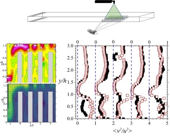
The normalized Reynolds stress distributions were considered to determine if there were any further significant turbulent features within the porous medium. These are plotted in Figure 8a–d for line-averaged normal stresses in the streamwise direction <u2> and wall-normal direction <v2>, and in Figure 8e,f for line-averaged shear stresses in the streamwise-wall-normal plane <−uv>. With a greater presence of solid boundaries along the stream, it is expected that the velocities normal to those surfaces will be suppressed more than the component parallel to the surface [50]. Hence, <v2> was found to be less than <u2>, suggesting an anisotropic turbulent field. It was also observed that some of the identifiable features of the turbulence intensities were present in the Reynolds normal stresses. The peak values were at approximately the same location as that of the turbulence intensities; additionally, the upstream columns of rods also showed some significant streamwise and wall-normal variations that were Reynolds number dependent. It is therefore reasonable to assume that some of the physics dictating the trends of the turbulence intensities and the Reynolds normal stresses are similar. The Reynolds shear stresses, however, were complex and very different from those reported by Manes et al. [18]. For the upstream rods, the Reynolds shear stresses generally declined with porous medium depth to a negative value, and then resulted in a null value. While the downstream rods showed a linear profile, there were distinctive changes in the off-midspan plane profiles. As these Reynolds shear stresses were produced by the mean shear in the streamwise-wall-normal plane within the turbulent flow, they recorded significant values at regions of substantial shear such as observed at regions close to the sidewalls.
3.1.3. Interfacial Flow
For a dense submerged canopy such as that under study, the drag due to the porous medium is expected to be larger than that of the lower wall. Thus, the discontinuity in drag that occurs at the interfacial edge will give rise to a region of shear that resembles a free shear layer with an inflection point near the interface [35]. The generation and propagation of K–H vortices from this shear layer suggest that the interface is a determinant of the degree of communication between the open and porous regional flows. Therefore, an understanding of the interfacial flow is integral to a proper view of the entire flow domain. The interfacial flow is known to be a function of several parameters including the specific permeability of the porous medium, average velocity within the porous medium, the velocity at that interface (i.e., the slip velocity), shear rate at the interface (i.e., Υ0 = dU/dy|y=h), and the channel’s local maximum velocity [51]. In this work, the interfacial flow was analyzed by focusing attention on measurements (or interpolations) of the slip velocity and its associated shear rate. The spatial variations of these select parameters were then studied with regard to changes in the bulk Reynolds numbers of the flow.
The reported slip velocity <Us> is defined as the line-averaged streamwise mean velocity at the plane tangent to the edges of the rods in most immediate contact with the open flow region (i.e., y = h). Particle image velocimetry measured velocities over a finite interrogation area whose center was not located exactly at this defined interface. Thus, it was not possible to provide the averaged slip velocities at the interface. Consequently, in this study, slip velocities could only be determined within interfacial location uncertainties of ±0.27 mm (which is half the size of an interrogation window). The line-averaged interfacial mean shear rate <Υ0> was also determined by using a curve of six or more streamwise velocity data points located at the region close to the interface. To assure some accuracy in the procedure, interpolations of the line-averaged data were first obtained. Differentiation of the curve was then performed smoothly over data points covering a distance of over 0.27 mm. The slip velocity and interfacial shear rates were then studied using three dimensionless parameters, namely <Us/Ub,p>, <Us/(Υ0 d)>, and <Us/Umax>. By using <Us/Ub,p> and <Us/(Υ0 d)>, the line-averaged slip velocities were respectively assessed in terms of the streamwise bulk flow within the porous medium <Ub,p> and the local penetration by the shear. On the other hand, by using <Us/Umax>, the relative effects of the overlying turbulent flow on the line-averaged slip velocities were determined. The results are summarized in Table 2 and Table 3.
The data in both tables show that the interfacial velocities dropped from their initial values in the upstream columns of rods, and then rose again with downstream rods. The rate at which shearing was applied increased to a peak just over the columns of rods, and subsequently declined as the region of obstruction was approached. The results also indicate that there were sharp flow reversals at the interfacial region, resulting in negative slip velocities (in some cases). Furthermore, there were negative shear rates at the interfaces. The flow reversals are consistent with some of the observations made regarding vector plots in Figure 4. While the negative shear rates were more confounding, they are still reasonable given that velocities higher than the slip velocities were identified just beneath the interface in Figure 3a. On the whole, it is remarkable that relative to the bulk velocity within the porous medium, the slip velocities were dependent on the spatial location and the Reynolds number, and not a constant value as observed by Suga et al. [7]. For <Us/(Υ0 d)> and <Us/Umax>, the slip velocities were also found to be greatest just after the most upstream rods. They also increased with Reynolds number. Across the span of the porous medium, however, both slip velocity and shear rates were dependent on the spatial location, and all the dimensionless parameters (<Us/Ub,p>, <Us/(Υ0 d)>, and <Us/Umax>) tended to be symmetrical about the midspan at the higher Reynolds number.
The overall conclusions regarding the interfacial flow are that while the slip velocities recorded in this work were largely substantial in value compared to the bulk flow within the porous medium, they were mostly a small fraction of the maximum velocity (≤6%). If the absolute value of <Us/Υ0> is a measure of the depth of penetration of the turbulent flow, then the <Us/(Υ0 d)> parameter determined tells us that the average depth of such infiltration through the interfacial zone is small (~7% of the rod diameter). However, this penetration is effective in creating some significant measure of porous flow just beneath the interface.
3.2. Flow Development over the Porous Wall
In this section, the results of the flow above the porous wall are presented and discussed. Consideration of the flow is limited to 1.25 h above the porous wall.
3.2.1. Boundary Layer Characteristics
Having considered the flow within the porous medium, attention is now turned to the overlying turbulent flow. To characterize the boundary layers of the selected line-averaged streamwise velocities, values of the maximum streamwise component of the mean velocity <Umax>, boundary layer thickness δ, streamwise location of the edge of the boundary layer (i.e., y/h value at 0.99<Umax>), displacement thickness δ*, momentum thickness θ*, Reynolds number based on momentum thickness and maximum velocity Reθ, and shape parameter H were determined from the line-averaged plots. These were obtained for selected locations, according to definitions of parameters given in Section 2.3. Apart from <Umax>, (which is summarized in Table 2 and Table 3), all the other relevant boundary layer values are presented in Table 4 and Table 5 and plotted in Figure 9 and Figure 10. It should be noted that for the convenience of analyses, the streamwise locations of the boundary layer data are taken as the center between the rods. Furthermore, the values of relevant entry flow boundary layer parameters are included in Figure 9 to show the effects of the porous medium on the flow.
By introducing the porous medium, a 21% blockage was created in the flow section, resulting in an increased acceleration of flow in the open region. Some of the results of this increment were a 27% to 32% rise in maximum velocities in the open region, and an upward shift in the location of the maximum flow. The latter can particularly be seen in Figure 9b, where the edge of the boundary layer changes substantially from ~1.3 h at the entry flow to ~1.5 h at the upstream rods. There were also significant reductions in δ and θ*, especially at the most upstream rods relative to the entry flow, following the characteristics associated with flows undergoing favorable pressure gradient changes [52,53]. However, due to the opposing effects of the porous medium (in generating significant mass flux deficit), similar reductions in δ* were resisted.
On the other hand, the porous boundary appeared to diffuse viscous effects into the mean turbulent flow in the open region. Thus, as the boundary layer developed over the porous medium, it thickened along the stream by about 90% at the trailing rods compared to its value over the leading rods. This boundary layer development also led to a monotonic increase in θ*, and an initial augmentation in δ*. It must be noted that both δ* and θ* are respectively indicators of the mass and momentum flux deficits. For the present tests, both parameters ultimately increased in value at the trailing rods (compared to that at the leading rods of the porous medium). Thus, it may be concluded that the current porous medium significantly enhanced mass and momentum deficit (by 42–102%). Consequently, with the 30% increase in maximum streamwise mean velocity, Reθ magnified much more significantly, and more prominently at the higher Reynolds number flow.
The relative effects of δ* and θ* in the flow arrangement are accounted for in the shape factor H trends indicated in Figure 9f and Table 4. For the entry flow, H compared well with previous results of turbulent flows over a smooth wall at zero pressure gradient and at similar Reθ [54]. However, along the streamwise direction on the porous wall, the values of H were found to be high, and characterized by two distinct zonal attributes. There was the first zone upstream of the porous medium, marked by a sharp increase in mass deficit flux compared to momentum deficit flux along the stream. There was also the second zone where in anticipation of lower flux deficits in the unobstructed flow downstream, the displacement thickness dropped sharply to a constant value while the momentum deficit flux continued to increase incrementally toward the trailing edge of the porous medium. Thus, H declined in the flow over the trailing rods of the porous medium. The value of H measured between columns 11 and 12 of the porous medium rods showed that the porous medium more than doubled the shape parameter of the boundary layer relative to the entry flow. This is predictable for obstructions in flow that generate higher drag characteristics such as that expected of the porous medium in the current flow arrangement [55].
Regarding spanwise changes in boundary layer characteristics, Figure 10 and Table 5 reveal variations were less dramatic compared to the streamwise changes. However, it is noteworthy from the data that lower flow speeds tended to display three-dimensional effects. In the current arrangement, this resulted in relative deviations that were no more than 16% of the value at the mid-plane. Such maximum deviations occurred at locations closer to the sidewalls.
3.2.2. Mean Velocities, Momentum Flux, and Vorticity
The mean velocity profiles in the streamwise directions are shown in the outer coordinates in Figure 11. As indicated in Section 3.1.3, there were flow reversals at the interface, specifically for mid-span line-averaged measurements between columns 4 and 5, and columns 8 and 9, respectively. The line averaged shear rates were also negative in value. All of these, along with the high H values observed in Figure 9 and Figure 10, point to complications in flow characteristics similar to those observed in adverse pressure gradient flows [55]. This behavior is possibly due to the intermittent pores on the surface of the porous medium.
The streamwise mean velocities were also critically examined to ascertain the validity of a logarithmic region in the flow profile over the porous wall during flow development. The associated friction velocities Uτ were also determined. In doing this, a modified form of the procedure outlined in Section 2.3 for rough wall turbulent flow [6,55,56] was followed. The normalized mean plots were matched with the following modified log law [42,55].
where U+ = U/Uτ and the von Kármán constant κ and logarithmic constants B were 0.41 and 5, respectively. It should be noted, however, that in this modified log law, the variable y+ = y Uτ/ν is defined as ( + yo) Uτ/ν. This is in line with the customary practice of rough wall experiments where the ‘roughness’ effects are considered in the definition of y. In the current setup, y is defined as the sum of the wall-normal distance from the top plane of the rods and a virtual origin . The parameter B+ is a ‘roughness’ function that measures the increase in local drag due to the presence of roughness elements on the surface [57]. Thus, it is seen as a downward shift of the log law profile of a comparable turbulent flow over a smooth wall. Following precedence then [6,55], the Clauser plot technique was used to simultaneously estimate Uτ and yo. Previous DNS results of turbulent flow over two-dimensional rods showed that at 1 < x/l < 9 (i.e., the initial developing flow region), yo/h ranges from 0.51 to 0.52 [58]. On this basis, an initial guess within this range was used. The optimized value of yo = 0.515 h yielded Uτ values listed in Table 4 and Table 5 with an uncertainty limit of ±10%. Selected streamwise mean velocity profiles in the inner coordinates are presented in Figure 12. Clearly, the associated roughness functions were high; indeed, they were found to range from 21 to 24 for the streamwise variation plots, and 18 to 23 for the spanwise variation plots. These values are much higher than what was indicated in other turbulent flows over rough surfaces [55,57,59], suggestive of the possibility of a different von Kármán constant than what was employed in this work.
From these assessments, it is evident that if existent, the logarithmic layer occupies a very limited region. The friction velocities Uτ (in Table 4 and Table 5) were substantially (9 to 18 times) higher over the porous surface compared to the entry flow over the smooth wall. As the flow over the porous surface developed along the stream, this friction velocity increased to a peak and declined thereafter. This is consistent with the trends seen for the displacement thickness observed in Figure 9, and mean velocity profiles in Figure 11. A similar trend in Uτ was reported in the simulations of Lee and Sung [58] for a turbulent flow over two-dimensional rods. However, in that work, their peak value was just about a quarter of the value recorded in this work. The higher values observed in the present tests stem from the increased drag due to the three-dimensional porous medium rod arrangement. The lateral deviations of Uτ, on the other hand, were insignificant considering the uncertainty limits.
Remarkably, the mean wall-normal profiles in Figure 13a,b were not negligible as often observed in turbulent flows over smooth walls of zero pressure gradient [55,58]. Indeed, in the flow over the first seven columns of rods, the maximum values were 5 to 12% of the line-averaged local maximum mean streamwise velocity. Compared with Figure 11, it is patent that the flow over those rods is three-dimensional, and that the wall-normal velocities contribute significantly to the mean momentum transport over the porous surface. Consequently, it is not surprising that mean momentum fluxes in Figure 13c,d were also significant. The high fluxes imply that they are also important factors in the production of shear stresses in those regions [57]. The dynamic roles of the mean wall-normal velocities and the momentum fluxes, however, declined downstream as the flow approached the unobstructed domain.
To illustrate the rotational regions of flow above the porous medium, the line-averaged mean spanwise vorticity <Ωz> (<∂V/∂x − ∂U/∂y>) distributions are plotted in Figure 14. They underscore the complex vorticial activity over the porous medium. These vortices are presumed to stem from Kelvin–Helmholtz (K–H) instabilities, and such are reported in other related studies [7,60]. In the current tests, the domination of these vortices were emphatic at the first seven columns of rods. For those domains, they were found to extend into increasing depth of the flow above the rods as they propagated through the flow. The location of the maximum vorticity also changed with the streamwise location. Compared with the flow through the porous medium, vortex motions over the rods were ~5 times more intense in magnitude, and more sustained. Moreover, the spatial variations along the span also showed that the presence of the side walls tended to heighten the vortex motions and more so at lower Reynolds number.
3.2.3. Turbulence Intensities, Reynolds Stresses, and Turbulent Energy
The turbulent intensities of the flow over the porous surface were also examined. They are plotted as line-averaged distributions in Figure 15. The results indicate that compared with the local mean streamwise velocities, the maximum streamwise and wall-normal turbulent intensities were ~25% and ~12%, respectively. The Reynolds number effects were also apparent in the wall-normal turbulent intensities. The maximum turbulent intensities measured in the flow above the porous medium were much higher than those measured at the entry flow and within the porous medium. Indeed, the relative proportions of the streamwise and wall-normal components were found to be higher than that recorded in previous works [7,60]. It is also worth noting that the variation of the wall-normal locations of the maximum streamwise turbulent intensities was relatively small compared with other mean flow quantities (e.g., momentum flux). This indicates that the maximum turbulent intensities were not so much a factor of the mass and momentum dynamics of the turbulent flow as the static attributes of the flow section. Thus, it is reasonable to conclude that the turbulent intensities are mostly due to the porous boundary condition, and specifically the structural arrangements of the porous material.
The profiles of the line-averaged Reynolds normal and shear stresses are shown in Figure 16. The Reynolds normal stresses were found to be qualitatively similar to the turbulent intensities. Thus, here also, as the wall-normal components were expected to be curbed by the porous wall, these values were smaller than the streamwise components. Additionally, the wall-normal locations of the maximum Reynolds normal stresses did not very much, consolidating the likelihood of the porous boundary being the main factor of influence of their magnitudes. The Reynolds shear stresses, on the other hand, were quite distinctive. The profiles of flow over the first six columns of rods had negative maximum values, while those over the downstream rods had positive maximum values. This observation of negative Reynolds shear stress measurements of turbulent flows over porous media is rare in the literature. However, it should be conceded that the literature has barely any record of turbulent boundary layer flow developments over porous media. Nevertheless, it is notable that Lee and Sung [58] reported negative Reynolds shear stresses in their direct numerical simulations of the turbulent boundary layer over a rod-roughened wall. These negative values were also specifically located over the most upstream two-dimensional rod. Hence, this feature is not totally out of the bounds of possibility. This phenomenon requires further study. However, it is also reasonable to note that if the negative mean momentum flux <−UV> is important in the production of the shear stress (as suggested in the streamwise momentum equation [57]), then large pockets of positive mean momentum flux <UV> (Figure 13c,d) may be a factor in the sign change in <−uv> [57].
To study large-scale anisotropy, ratios of the Reynold stresses were analyzed. The plots are presented in Figure 17. As shown, close to the porous boundary, the ratio of the normal stresses tended to decay and flatten to values other than unity. Further away from the walls, they increased to ~0.5. The ratios of the Reynolds shear stress and the normal stress, however, were complex. As the flow developed downstream, the ratio of the Reynolds shear stress and the streamwise component of the normal stress varied throughout the flow, with Reynolds effects apparent in the spanwise planes. As expected, the effects of negative Reynolds shear stresses were also present in the upstream rods. It has been reported that some researchers (e.g., Suga [61]) have been able to develop turbulence models for fully developed flows over porous media with varying degrees of success. The results showed herein, however, indicate that the use of models (e.g., k-ε and k-ω) that assume local isotropy do not apply to turbulent flows over compact porous media as tested in this work.
In another consideration, the turbulent kinetic energy k was assessed. As the current measurement system is planar, the Reynolds normal stress in the spanwise direction w2 could not be measured directly. Thus, k was estimated as 0.75 (u2 + v2). The normalized line-averaged profiles are shown in Figure 18. As the streamwise component of the Reynolds normal stress is the dominant contributor of k, the profiles are qualitatively similar to the streamwise Reynolds normal stress distributions in Figure 16. Clearly, there is significant turbulent kinetic energy at the domain where intense vorticial activity is prevalent. The ratio of the Reynolds shear stress to the kinetic energy is an important parameter that is used to calibrate turbulence model coefficient Ck [62,63]. This constant (also called Townsend’s structure parameter, <−uv/(2k)> is used in the Kolmogorov–Prandtl expression associated with the eddy viscosity vT (=Ck k/L, where L is a length scale). De Lemos [63] suggested a constant for turbulent flow over porous media. However, Figure 19 indicates that this coefficient may vary from ~−0.3 to 0.1 depending on the wall-normal location above the porous medium.
4. Conclusions
The focus of the present work was the investigation of a turbulent flow through and over a compact porous medium. This research was conducted to measure the development of the flow over the porous boundary, the penetration of the turbulent flow into the porous domain, the attendant three-dimensional effects, and Reynolds number effects. These objectives were achieved by conducting particle image velocimetry measurements in a test section with turbulent flow through and over a compact model porous medium of porosity 85%, and filling fraction of 21%. The porous medium model was made of a square array of cylindrical rods of twelve columns and nine rows. The tests were carried out at Reynolds numbers (based on the bulk flow through the entire channel, and the depth of the channel) = 14,338 and 24,510.
Overall, this work indicates that the flow through and over a compact porous medium exhibits phenomenon different and somewhat complex compared to that associated with fully developed domains. The flow above the compact porous medium showed a complex flow development pattern with the boundary layer thickening along the stream by about 90% at the trailing rods, increasing monotonically in momentum thickness, and growing non-monotonically in displacement thickness and shape parameter. The spanwise variations, on the other hand, were no more than 16% from the value at the mid-plane. The mean velocities showed that if existent, the logarithmic layer occupied a very limited region. The friction velocities were 9 to 18 times higher over the porous surface compared to the entry flow over the smooth wall. There were significant complex vorticial activities over the porous medium, extending into an increasing depth of the flow above the rods as they propagate through the flow. The ratios of the Reynolds stresses showed a complex large-scale anisotropy in the flow over the porous medium. The implication then is that the use of turbulence models that assume local isotropy through and over porous media may not apply to turbulent flows over compact porous media. At the interface between the porous medium and the overlying turbulent flow, the slip velocities were no more than 6% of the maximum velocity. The shear rate obtained indicates that the average depth of such infiltration through the interfacial zone was only about 7% of the rod diameter. For the flow through the porous medium, the results showed that the streamwise velocities, in particular, had variations with negative gradients close to the lower wall and in the planes outside of the midspan. Pockets of variant sizes of the mean spanwise vortices appeared to be propagated from regions of shear through the porous medium, at the edge of the most upstream porous medium rods, and the interfacial region.
This work provides useful insight into the physics of flow pertinent to natural and industrial scenarios such as terrestrial or aquatic canopy flows over regions with small/confined arrangements of sparse vegetation, and flows associated with pin-fin arrays of rods for heat transfer enhancement. The data may serve as a useful resource for developing and validating numerical models.
Funding
This work was funded by the C Graydon and Mary E Rogers Fellowship.
Institutional Review Board Statement
Not applicable.
Informed Consent Statement
Not applicable.
Data Availability Statement
The data presented in this study are available on request from the corresponding author.
Acknowledgments
The author acknowledges with gratitude the financial support of Bucknell University through the C Graydon and Mary E Rogers Fellowship. The work of Owen Schiele in helping to complete the experiments, is also gratefully acknowledged.
Conflicts of Interest
The author declares no conflict of interest. The funders had no role in the design of the study; in the collection, analyses, or interpretation of data; in the writing of the manuscript, or in the decision to publish the results.
Nomenclature
| English | |
| A | Measured parameter: Test condition at ReH = 14,338 |
| B | Test condition at reh = 24,510; logarithmic law constant |
| B+ | Roughness function |
| b | Location in the wall-normal direction |
| C | Column |
| Cf | Skin-friction coefficient = 2 (Uτ/Ue)2 |
| Ck | Townsend parameter = <−uv/(2k)> |
| d | Nominal diameter of rods (mm) |
| g | Acceleration due to gravity (m/s) |
| h | Average height of rods (mm) |
| H | Channel depth (mm); shape factor = δ*/θ* |
| k | Turbulent kinetic energy ≈ 0.75 (u2 + v2) (m2 s−2) |
| L | Length scale |
| l | Distance between centers of adjacent rods (mm) |
| n | Column number |
| P | Plane |
| R | Row, location in the spanwise direction |
| ReH | Bulk Reynolds number = ubh/ν |
| Reθ | Reynolds number based on momentum thickness and maximum velocity |
| U | Mean (time-averaged) streamwise velocity (m s−1) |
| u | Streamwise turbulence intensity (m s−1) |
| u2 | Streamwise Reynolds normal stress (m2 s−2) |
| Ub | Bulk velocity in the channel (m s−1) |
| Ub,p | Average streamwise velocity within the porous region (m s−1) |
| Ue | Maximum velocity of entry flow (m s−1) |
| Us | Streamwise mean slip velocity (m s−1) |
| Umax | Maximum time-averaged streamwise velocity in the flow section with a porous medium model (m s−1) |
| Uτ | Friction velocity (m s−1) |
| U+ | Time-averaged streamwise velocity in inner coordinates = U/Uτ |
| UV | Mean momentum flux (m2 s−2) |
| −uv | Reynolds shear stress (m2 s−2) |
| V | Mean (time-averaged) wall-normal velocity (m s−1) |
| v | Wall-normal turbulence intensity (m s−1) |
| v2 | Wall-normal Reynolds normal stress (m2 s−2) |
| vs | Settling velocity (m s−1) |
| x | Streamwise direction; streamwise distance (m) |
| y | Wall-normal direction; wall-normal distance (m) |
| yo | Virtual origin |
| y* | Wall-normal distance from the top plane of the rods (m) |
| y+ | Wall-normal direction in inner coordinates = y Uτ/ν |
| z | Spanwise direction; spanwise distance (m) |
| Greek | |
| δ | Boundary layer thickness (m) |
| δ* | Displacement thickness (m) |
| ε | Porosity |
| η | Kolmogorov length scale ≈ 3ν/Uτ (m) |
| θ* | Momentum thickness (m) |
| κ | Von Kármán constant |
| λ | Taylor microscale ≈ √15(Ueη2)/ν (m) |
| ν | Kinematic viscosity (m2 s−1) |
| ρf | Fluid density (kg m−3) |
| ρp | Particle density (kg m−3) |
| τf | Viscous time scale = ν/Uτ2 (s) |
| τR | Response time (s) |
| Υ0 | Shear rate at the interface = dU/dy|y=h (s−1) |
| Ωz | Mean spanwise vorticity = ∂V/∂x − ∂U/∂y (s−1) |
| Other Symbols/Acronyms | |
| < > | Line-averaged parameter |
| K-H | Kelvin–Helmholtz |
| Nd:YAG | Neodymium: Yttrium Aluminum Garnet |
| PIV | Particle image velocimetry |
| RIM | Refractive index matching |
References
- Beavers, G.S.; Joseph, D.D. Boundary conditions at a naturally permeable wall. J. Fluid Mech. 1967, 30, 197–207. [Google Scholar] [CrossRef]
- Neale, G.; Nader, W. Practical significance of Brinkman’s extension of Darcy’s law: Coupled parallel flows within a channel and a bounding porous medium. Can. J. Chem. Eng. 1974, 52, 475–478. [Google Scholar] [CrossRef]
- Vafai, K.; Kim, S.J. Forced convection in a channel filled with a porous medium: An exact solution. ASME J. Heat Transf. 1989, 111, 1103–1106. [Google Scholar] [CrossRef]
- Arthur, J.K.; Ruth, D.W.; Tachie, M.F. PIV measurements of flow through a model porous medium with varying boundary conditions. J. Fluid Mech. 2009, 629, 343–374. [Google Scholar] [CrossRef]
- Florens, E.; Eiff, O.; Moulin, F. Defining the roughness sublayer and its turbulence statistics. Exp. Fluids 2013, 54, 1500. [Google Scholar] [CrossRef] [Green Version]
- Kim, T.; Blois, G.; Best, J.L.; Christensen, K.T. Experimental study of turbulent flow over and within cubically packed walls of spheres: Effects of topography, permeability and wall thickness. Int. J. Heat Fluid Flow 2018, 73, 16–29. [Google Scholar] [CrossRef]
- Suga, K.; Okazaki, Y.; Ho, U.; Kuwata, Y. Anisotropic wall permeability effects on turbulent channel flows. J. Fluid Mech. 2018, 855, 983–1016. [Google Scholar] [CrossRef]
- Arthur, J.K. PIV study of flow through and over porous media at the onset of inertia. Adv. Water Resour. 2020, 146, 103793. [Google Scholar] [CrossRef]
- Lyu, W.; Wang, X. Stokes–Darcy system, small-Darcy-number behaviour and related interfacial conditions. J. Fluid Mech. 2021, 922, 509. [Google Scholar] [CrossRef]
- Angot, P.; Goyeau, B.; Ochoa-Tapia, J.A. A nonlinear asymptotic model for the inertial flow at a fluid-porous interface. Adv. Water Resour. 2021, 149, 103798. [Google Scholar] [CrossRef]
- Sengupta, S.; De, S. Effect of the transition layer on the stability of a fluid-porous configuration: Impact on power-law rheology. Phys. Rev. Fluids 2021, 6, 063902. [Google Scholar] [CrossRef]
- Hester, E.T.; Cardenas, M.B.; Haggerty, R.; Apte, S.V. The importance and challenge of hyporheic mixing. Water Resour. Res. 2017, 53, 3565–3575. [Google Scholar] [CrossRef] [Green Version]
- Ghisalberti, M.; Nepf, H. Shallow flows over a permeable medium: The hydrodynamics of submerged aquatic canopies. Transp. Porous Media 2009, 78, 309–326. [Google Scholar] [CrossRef]
- Belcher, S.E.; Finnigan, J.J.; Harman, I.N. Flows through forest canopies in complex terrain. Ecol. Appl. 2008, 18, 1436–1453. [Google Scholar] [CrossRef]
- Segalini, A. Linearized simulation of flow over wind farms and complex terrains. Philos. Trans. R. Soc. A Math. Phys. Eng. Sci. 2017, 375, 20160099. [Google Scholar] [CrossRef] [PubMed]
- Uzol, O.; Camci, C. Heat transfer, pressure loss and flow field measurements downstream of staggered two-row circular and elliptical pin fin arrays. J. Heat Transf. 2005, 127, 458–471. [Google Scholar] [CrossRef]
- Prescott, P.J.; Incropera, F.P. The effect of turbulence on solidification of a binary metal alloy with electromagnetic stirring. ASME 1995, 117, 716–724. [Google Scholar] [CrossRef]
- Manes, C.; Pokrajac, D.; McEwan, I.; Nikora, V. Turbulence structure of open channel flows over permeable and impermeable beds: A comparative study. Phys. Fluids 2009, 21, 125109. [Google Scholar] [CrossRef] [Green Version]
- Raupach, M.; Thom, A.S. Turbulence in and above plant canopies. Annu. Rev. Fluid Mech. 1981, 13, 97–129. [Google Scholar] [CrossRef]
- Finnigan, J. Turbulence in plant canopies. Annu. Rev. Fluid Mech. 2000, 32, 519–571. [Google Scholar] [CrossRef]
- Ghisalberti, M.; Nepf, H.M. Mixing layers and coherent structures in vegetated aquatic flows. J. Geophys. Res. Ocean. 2002, 107, 3–11. [Google Scholar] [CrossRef]
- Ruff, J.F.; Gelhar, L.W. Turbulent shear flow in porous boundary. J. Eng. Mech. Div. 1972, 98, 975–991. [Google Scholar] [CrossRef]
- Zagni, A.F.; Smith, K.V. Channel flow over permeable beds of graded spheres. J. Hydraul. Div. 1976, 102, 207–222. [Google Scholar] [CrossRef]
- Vollmer, S.; de los Santos Ramos, F.; Daebel, H.; Kühn, G. Micro scale exchange processes between surface and subsurface water. J. Hydrol. 2002, 269, 3–10. [Google Scholar] [CrossRef]
- Breugem, W.P.; Boersma, B.J.; Uittenbogaard, R.E. The influence of wall permeability on turbulent channel flow. J. Fluid Mech. 2006, 562, 35–72. [Google Scholar] [CrossRef] [Green Version]
- Pokrajac, D.; Manes, C. Velocity measurements of a free-surface turbulent flow penetrating a porous medium composed of uniform-size spheres. Transp. Porous Media 2009, 78, 367–383. [Google Scholar] [CrossRef]
- Nikora, V.; McEwan, I.; McLean, S.; Coleman, S.; Pokrajac, D.; Walters, R. Double-averaging concept for rough-bed open-channel and overland flows: Theoretical background. J. Hydraul. Eng. 2007, 133, 873–883. [Google Scholar] [CrossRef]
- Suga, K.; Nakagawa, Y.; Kaneda, M. Spanwise turbulence structure over permeable walls. J. Fluid Mech. 2017, 822, 186–201. [Google Scholar] [CrossRef]
- Suga, K.; Matsumura, Y.; Ashitaka, Y.; Tominaga, S.; Kaneda, M. Effects of wall permeability on turbulence. Int. J. Heat Fluid Flow 2010, 31, 974–984. [Google Scholar] [CrossRef]
- Pokrajac, D.; Manes, C.; McEwan, I. Peculiar mean velocity profiles within a porous bed of an open channel. Phys. Fluids 2007, 19, 098109. [Google Scholar] [CrossRef] [Green Version]
- Sharma, A.; García-Mayoral, R. Turbulent flows over dense filament canopies. J. Fluid Mech. 2020, 888, A2. [Google Scholar] [CrossRef] [Green Version]
- Szepessy, S.; Bearman, P.W. Aspect ratio and end plate effects on vortex shedding from a circular cylinder. J. Fluid Mech. 1992, 234, 191–217. [Google Scholar] [CrossRef]
- Ostanek, J.K.; Thole, K.A. Effects of varying streamwise and spanwise spacing in pin-fin arrays. Turbo Expo Power Land Sea Air 2012, 44700, 45–57. [Google Scholar]
- Anderson, C.D.; Lynch, S.P. Time-resolved stereo PIV measurements of the horseshoe vortex system at multiple locations in a low-aspect-ratio pin–fin array. Exp. Fluids 2016, 57, 5. [Google Scholar] [CrossRef]
- Nepf, H.M. Flow and transport in regions with aquatic vegetation. Annu. Rev. Fluid Mech. 2012, 44, 123–142. [Google Scholar] [CrossRef] [Green Version]
- Moroni, M.; Cushman, J.H. Statistical mechanics with three-dimensional particle tracking velocimetry experiments in the study of anomalous dispersion. II Experiments. Phys. Fluids 2001, 13, 81–91. [Google Scholar] [CrossRef]
- Huang, A.Y.; Huang, M.Y.; Capart, H.; Chen, R. Optical measurements of pore geometry and fluid velocity in a bed of irregularly packed spheres. Exp. Fluids 2008, 45, 309–321. [Google Scholar] [CrossRef]
- Raffel, M.; Willert, C.E.; Scarano, F.; Kähler, C.J.; Wereley, S.T.; Kompenhans, J. Particle Image Velocimetry: A Practical Guide; Springer: Berlin/Heidelberg, Germany, 2018. [Google Scholar]
- Samimy, M.; Lele, S.K. Motion of particles with inertia in a compressible free shear layer. Phys. Fluids A Fluid Dyn. 1991, 3, 1915–1923. [Google Scholar] [CrossRef] [Green Version]
- Prasad, A.K. Particle image velocimetry. Curr. Sci. 2000, 79, 51–60. [Google Scholar]
- Wieneke, B. PIV uncertainty quantification from correlation statistics. Meas. Sci. Technol. 2015, 26, 074002. [Google Scholar] [CrossRef]
- Kadivar, M.; Tormey, D.; McGranaghan, G. A review on turbulent flow over rough surfaces: Fundamentals and theories. Int. J. Thermofluids 2021, 10, 100077. [Google Scholar] [CrossRef]
- Millikan, C.B. A critical discussion of turbulent flow in channels and circular tubes. In Proceedings of the 5th International Congress on Applied Mechanics, Wiley, New York, NY, USA, 12–16 September 1938; pp. 386–392. [Google Scholar]
- Durst, F.; Fischer, M.; Jovanović, J.; Kikura, H. Methods to set up and investigate low Reynolds number, fully developed turbulent plane channel flows. J. Fluids Eng. 1998, 120, 496–503. [Google Scholar] [CrossRef]
- Johansson, A.V.; Alfredsson, P.H. Effects of imperfect spatial resolution on measurements of wall-bounded turbulentbx shear flows. J. Fluid Mech. 1983, 137, 409–421. [Google Scholar] [CrossRef]
- He, X.; Apte, S.V.; Finn, J.R.; Wood, B.D. Characteristics of turbulence in a face-centred cubic porous unit cell. J. Fluid Mech. 2019, 873, 608–645. [Google Scholar] [CrossRef]
- Koch, D.L.; Ladd, A.J.C. Moderate Reynolds number flows through periodic and random arrays of aligned cylinders. J. Fluid Mech. 1997, 349, 31–66. [Google Scholar] [CrossRef]
- Hill, R.J.; Koch, D.L. The transition from steady to weakly turbulent flow in a close-packed ordered array of spheres. J. Fluid Mech. 2002, 465, 59–97. [Google Scholar] [CrossRef]
- Suekane, T.; Yokouchi, Y.; Hirai, S. Inertial flow structures in a simple-packed bed of spheres. AIChE J. 2003, 49, 10–17. [Google Scholar] [CrossRef]
- Bernard, P.S. Turbulent Fluid Flow; John Wiley & Sons: Hoboken, NJ, USA, 2019. [Google Scholar]
- Arthur, J.K. Flow through and over Model Porous Media with or without Inertial Effects; University of Manitoba: Winnipeg, MB, Canada, 2012. [Google Scholar]
- Escudier, M.P.; Abdel-Hameed, A.; Johnson, M.W.; Sutcliffe, C.J. Laminarisation and re-transition of a turbulent boundary layer subjected to favourable pressure gradient. Exp. Fluids 1998, 25, 491–502. [Google Scholar] [CrossRef]
- Narayanan, M.A.B.; Ramjee, V. On the criteria for reverse transition in a two-dimensional boundary layer flow. J. Fluid Mech. 1969, 35, 225–241. [Google Scholar] [CrossRef]
- Purtell, L.P.; Klebanoff, P.S.; Buckley, F.T. Turbulent boundary layer at low Reynolds number. Phys. Fluids 1981, 24, 802–811. [Google Scholar] [CrossRef]
- Tachie, M.F. Particle image velocimetry study of turbulent flow over transverse square ribs in an asymmetric diffuser. Phys. Fluids 2007, 19, 065106. [Google Scholar] [CrossRef]
- Schultz, M.P.; Flack, K.A. Outer layer similarity in fully rough turbulent boundary layers. Exp. Fluids 2005, 38, 328–340. [Google Scholar] [CrossRef]
- Ashrafian, A.; Andersson, H.I.; Manhart, M. DNS of turbulent flow in a rod-roughened channel. Int. J. Heat Fluid Flow 2004, 25, 373–383. [Google Scholar] [CrossRef]
- Lee, S.; Sung, H.J. Direct numerical simulation of the turbulent boundary layer over a rod-roughened wall. J. Fluid Mech. 2007, 584, 125–146. [Google Scholar] [CrossRef] [Green Version]
- Tachie, M.F.; Shah, M.K. Favorable pressure gradient turbulent flow over straight and inclined ribs on both channel walls. Phys. Fluids 2008, 20, 095103. [Google Scholar] [CrossRef]
- Suga, K.; Mori, M.; Kaneda, M. Vortex structure of turbulence over permeable walls. Int. J. Heat Fluid Flow 2011, 32, 586–595. [Google Scholar] [CrossRef]
- Suga, K. Understanding and modelling turbulence over and inside porous media. Flow Turbul. Combust. 2016, 96, 717–756. [Google Scholar] [CrossRef]
- Pedras, M.H.; de Lemos, M.J. Macroscopic turbulence modeling for incompressible flow through undeformable porous media. Int. J. Heat Mass Transf. 2001, 44, 1081–1093. [Google Scholar] [CrossRef]
- de Lemos, M.J. Turbulent kinetic energy distribution across the interface between a porous medium and a clear region. Int. Commun. Heat Mass Transf. 2005, 32, 107–115. [Google Scholar] [CrossRef]
Figure 1.
Schematics showing (a) the model test channel and PIV system; (b) front view showing details of porous arrangements in the test channel as well as streamwise planar coverage of PIV measurements (shown using blue and boxes with dashed line boundaries); and (c) top view of the porous model arrangement in the model test channel with green lines indicating lateral locations of measurement with the laser sheet. All numeric dimensions are in millimeters.

Figure 2.
Boundary layer profiles of entry flow in the (a) outer and (b) inner coordinates for the two test cases. Plots in (b,c) are the turbulence intensities in the streamwise direction (u), and turbulence intensities in the wall-normal direction (v). Note that Ue is the maximum velocity of the entry flow streamwise component of the mean velocity (U); U+ = U/Uτ where Uτ is the friction velocity, and y+ = y Uτ/ν where ν is the kinematic viscosity of the fluid. Note that the legend shown in (a) applies to (b–d).

Figure 3.
Parameters <U/Umax> and <V/Umax> are respectively line-averaged streamwise and wall-normal components of the mean velocity normalized by the maximum localline-averaged streamwise mean velocity in both open and porous regions. Here, the profiles for the flow within the porous medium are shown. Staggered plots (a,c) show the streamwise variations whereas (b,d) demonstrate the spanwise variations. The denominations C and R respectively stand for columns and rows, and are illustrated in Figure 1. Black-filled boxes are the results for Test A, and red-open boxes are the results for Test B.

Figure 4.
Vector plots for the selected rods at (a) z = 0 in Test A; (b) z = 0 in Test B; (c) z = l in Test B; (d) z = −l in Test B. Note that for each plot, gray-filled boxes indicate locations of porous medium rods. Vectors have also been skipped to maintain clarity.
Figure 4.
Vector plots for the selected rods at (a) z = 0 in Test A; (b) z = 0 in Test B; (c) z = l in Test B; (d) z = −l in Test B. Note that for each plot, gray-filled boxes indicate locations of porous medium rods. Vectors have also been skipped to maintain clarity.

Figure 5.
Vector plots with streamlines superimposed for selected rods at (a,b) z = l/2 in Test A; (c,d) z = l/2 in Test B; (e,f) z = −l/2 in Test A; (g,h) z = −l/2 in Test B. Note that for each plot, dashed lines indicate locations of porous medium rods. Vectors and streamlines have also been skipped in order to maintain clarity and to highlight features.

Figure 6.
Iso-contours of mean spanwise vorticity Ωz = ∂V/∂x − ∂U/∂y normalized by the maximum entry flow velocity and the rod diameter. Plots (a–c) are results of measurements taken at z = l/2 in Test A. Plots (d–f) were extracted from measurements taken at z = l/2 in Test B. Plots (g–i) were extracted from measurements taken at z = −l/2 in Test B. Note that for each plot, dashed lines indicate locations of porous medium rods.

Figure 7.
Parameters <u/Umax> and <v/Umax> are respectively line-averaged streamwise and wall-normal turbulence intensities normalized by the maximum local line-averaged streamwise mean velocity in both open and porous regions. Here, the profiles for the flow within the porous medium are shown. Staggered plots (a,c) show the streamwise variations whereas (b,d) demonstrate the spanwise variations. The denominations C and R respectively stand for columns and rows, and are illustrated in Figure 1. Black-filled boxes are for results for Test A, and red-open boxes are for results for Test B.

Figure 8.
Turbulence quantities <u2/Umax2>, <v2/Umax2>, and <−uv/Umax2> are respectively line-averaged streamwise Reynolds normal stress, wall-normal Reynolds normal stress, and Reynolds shear stress in the streamwise-wall-normal plane, normalized by the maximum local line-averaged streamwise mean velocity in both open and porous regions. Here, the profiles for the flow within the porous medium are shown. Staggered plots (a,c,e) show the streamwise variations whereas (b,d,f) demonstrate the spanwise variations. The denominations C and R respectively stand for columns and rows, and are illustrated in Figure 1. Black-filled boxes are the results for Test A, and red-open boxes are the results for Test B.

Figure 9.
Streamwise variation of (a) boundary layer thickness; (b) location of the edge of the boundary layer (i.e., y/h values at 0.99<Umax>); (c) displacement thickness; (d) momentum thickness; (e) Reynolds number based on momentum thickness and maximum velocity; and (f) shape parameter. Note that the legend showed in (a) applies to (b–f).

Figure 10.
Spanwise variation of (a) boundary layer thickness; (b) location of the edge of the boundary layer (y/h values at 0.99<Umax>); (c) displacement thickness; (d) momentum thickness; (e) Reynolds number based on momentum thickness and maximum velocity; and (f) shape parameter. Note that the legend showed in (a) applies to (b–f).

Figure 11.
Turbulence quantity <U/Umax> is the line-averaged mean streamwise velocity normalized by the maximum local line-averaged streamwise mean velocity in open and porous regions. Here, the profiles for the flow in the open region are shown. Staggered plots in (a) show the streamwise variations whereas (b) demonstrate the spanwise variations. The denominations C and R respectively stand for columns and rows, and are illustrated in Figure 1. Black-filled boxes are the results for Test A, and red-open boxes are the results for Test B.

Figure 12.
Mean streamwise line-averaged velocity profiles in inner coordinates for selected Test B conditions. Plots in (a) show streamwise variations compared with entry flow. Plots in (b) show spanwise variations compared with entry flow. The solid red line represents log law (Equation (2)). The red dashed line represents the law of the wall U+ = y+. Other solid lines represent modified log law for rough walls (Equation (3)). The denominations C and R respectively stand for columns and rows, and are illustrated in Figure 1. Black-filled boxes are the results for Test A, and red-open boxes are the results for Test B.

Figure 13.
Turbulence quantities <V/Umax>, and <UV/Umax2> are respectively line-averaged mean wall-normal velocity, and momentum flux, normalized by the local maximum line-averaged streamwise mean velocity in open and porous regions. Here, the profiles for the flow in the open region are shown. Staggered plots (a,c) show the streamwise variations whereas (b,d) demonstrate the spanwise variations. The denominations C and R respectively stand for columns and rows, and are illustrated in Figure 1. Black-filled boxes are the results for Test A, and red-open boxes are for results for Test B.

Figure 14.
Line-averaged mean spanwise vorticity <Ωz > = <∂V/∂x − ∂U/∂y> plots normalized by the ratio of the local maximum line-averaged streamwise mean velocity and rod diameter. Plots in (a) are staggered distributions along the stream, and those in (b) are staggered across the span in the open region. The denominations C and R respectively stand for columns and rows, and are illustrated in Figure 1. Black-filled boxes are the results for Test A, and red-open boxes are the results for Test B.

Figure 15.
Parameters <u/Umax> and <v/Umax> are respectively line-averaged streamwise and wall-normal turbulence intensities normalized by the local maximum line-averaged streamwise mean velocity in both open and porous regions. Here, the profiles for the flow in the open region are shown. Staggered plots (a,c) show the streamwise variations whereas (b,d) demonstrate the spanwise variations. The denominations C and R respectively stand for columns and rows, and are illustrated in Figure 1. Black-filled boxes are the results for Test A, and red-open boxes are the results for Test B.

Figure 16.
Turbulence quantities <u2/Umax2>, <v2/Umax2>, and <−uv/Umax2> are respectively line-averaged streamwise Reynolds normal stress, wall-normal Reynolds normal stress, and Reynolds shear stress in the streamwise-wall-normal plane, normalized by the local maximum line-averaged streamwise mean velocity in both open and porous regions. Here, the profiles for the flow in the open region are shown. Staggered plots (a,c,e) show the streamwise variations whereas (b,d,f) demonstrate the spanwise variations. The denominations C and R respectively stand for columns and rows, and are illustrated in Figure 1. Black-filled boxes are the results for Test A, and red-open boxes are the results for Test B.


Figure 17.
Reynolds stress ratios for the flow in the open region are shown. Staggered plots (a,c,e) show the streamwise variations whereas (b,d,f) demonstrate the spanwise variations. The denominations C and R respectively stand for columns and rows, and are illustrated in Figure 1. Black-filled boxes are the results for Test A, and red-open boxes are the results for Test B.


Figure 18.
Turbulent kinetic energy profiles for the flow in the open region are shown. The plots are shown as normalized by the local maximum line-averaged streamwise mean velocity in both open and porous regions. Staggered plots (a) show the streamwise variations whereas staggered plots (b) demonstrate the spanwise variations. The denominations C and R respectively stand for columns and rows, and are illustrated in Figure 1. Black-filled boxes are the results for Test A, and red-open boxes are the results for Test B.

Figure 19.
Evaluation of Townsend structure parameter for the flow in the open region is shown. Staggered plots (a) show the streamwise variations whereas staggered plots (b) demonstrate the spanwise variations. The denominations C and R respectively stand for columns and rows, and are illustrated in Figure 1. Black-filled boxes are the results for Test A, and red-open boxes are the results for Test B.


Table 1.
Summary of geometric parameters of test model, boundary layer parameters of entry flow, and friction parameters of entry flow.
Table 1.
Summary of geometric parameters of test model, boundary layer parameters of entry flow, and friction parameters of entry flow.
| Geometric Parameters of Test Model | ||||||
|---|---|---|---|---|---|---|
| Porous Medium Depth h (mm) | Channel Depth H (mm) | Filling Fraction h/H | Rod Diameter of Porous Medium d (mm) | Distance between Adjacent Rod Centers l (mm) | Porosity of Porous Medium ε | |
| 9.06 | 43 | 0.21 | 3.18 | 7.19 | 0.85 | |
| Boundary Layer Parameters of Entry Flow | ||||||
| Test Label | Bulk Velocity Ub (m/s) | Maximum Velocity Ue (m/s) | Boundary Layer Thickness δ (mm) | Displacement Thickness δ* (mm) | Momentum Thickness θ* (mm) | Shape Factor H |
| A | 0.3347 | 0.3927 | 12.24 | 1.87 | 1.17 | 1.60 |
| B | 0.5721 | 0.6453 | 10.78 | 1.38 | 0.94 | 1.48 |
| Friction Parameters of Entry Flow | ||||||
| Test Label | Friction Velocity Uτ (m/s) | Skin Friction Coefficient Cf | Bulk Reynolds Number ReH | Momentum Thickness Reynolds Number Reθ | ||
| A | 0.0145 | 0.003 | 14,338 | 461 | ||
| B | 0.0222 | 0.002 | 24,510 | 604 | ||
Table 2.
Summary results of porous media parameters showing streamwise variation in midspan plane.
| Test | Parameter | Averaged Value at Location in Porous Medium | ||||
|---|---|---|---|---|---|---|
| A | Column 1 and 2 (C1–2) | Column 4 and 5 (C4–5) | Column 6 and 7 (C6–7) | Column 8 and 9 (C8–9) | Column 11 and 12 (C11–12) | |
| <Ub,p> (mm/s) | 1.38 × 10⁻³ | 2.97 × 10⁻³ | 3.99 × 10⁻³ | 9.49 × 10⁻⁴ | 8.46 × 10⁻⁶ | |
| <Us> (m/s) | 4.32 × 10⁻³ | −5.60 × 10⁻⁴ | 2.44 × 10⁻⁴ | −9.49 × 10⁻⁴ | 2.61 × 10⁻³ | |
| Line-Averaged Shear Rate <ϒ0 >(1/s) | −1.41 × 101 | 4.83 × 10⁻¹ | 4.61 × 100 | −1.52 × 100 | −1.02 × 101 | |
| <Umax> (m/s) | 4.19 × 10⁻¹ | 4.36 × 10⁻¹ | 4.46 × 10⁻¹ | 4.50 × 10⁻¹ | 4.54 × 10⁻¹ | |
| Percentage Flow in Porous Medium (%) | 1.09 × 10⁻¹ | 2.33 × 10⁻¹ | 3.17 × 10⁻¹ | 7.13 × 10⁻² | 6.29 × 10⁻⁴ | |
| <Us/Ub,p> | 3.13 × 100 | −1.88 × 10⁻¹ | 6.12 × 10⁻² | −1.00 × 100 | 3.08 × 10² | |
| <Us/(ϒ0d)> | −9.61 × 10⁻² | −3.64 × 10⁻¹ | 1.67 × 10⁻² | 1.96 × 10⁻¹ | −8.07 × 10⁻² | |
| <Us/Umax> | 1.03 × 10⁻² | −1.28 × 10⁻³ | 5.47 × 10⁻⁴ | −2.11 × 10⁻³ | 5.75 × 10⁻³ | |
| B | <Ub,p> (m/s) | 8.68 × 10⁻⁴ | 4.66 × 10⁻³ | 6.57 × 10⁻³ | 1.29 × 10⁻³ | 8.29 × 10⁻⁴ |
| <Us> (m/s) | 3.87 × 10⁻² | 1.31 × 10⁻² | 4.23 × 10⁻⁴ | 1.61 × 10⁻² | 2.17 × 10⁻² | |
| Line-Averaged Shear Rate <ϒ0 >(1/s) | −8.65 × 101 | −1.07 × 101 | −1.72 × 100 | −5.10 × 101 | −5.93 × 101 | |
| <Umax> (m/s) | 7.02 × 10⁻¹ | 7.22 × 10⁻¹ | 7.38 × 10⁻¹ | 7.47 × 10⁻¹ | 7.54 × 10⁻¹ | |
| Percentage Flow in Porous Medium (%) | 3.89 × 10⁻² | 2.06 × 10⁻¹ | 2.90 × 10⁻¹ | 5.51 × 10⁻² | 3.51 × 10⁻² | |
| <Us/Ub,p> | 4.46 × 101 | 2.80 × 100 | 6.44 × 10⁻² | 1.24 × 101 | 2.62 × 101 | |
| <Us/(ϒ0d)> | −1.41 × 10⁻¹ | −3.83 × 10⁻¹ | −7.72 × 10⁻² | −9.91 × 10⁻² | −1.15 × 10⁻¹ | |
| <Us/Umax> | 5.52 × 10⁻² | 1.81 × 10⁻² | 5.73 × 10⁻⁴ | 2.15 × 10⁻² | 2.88 × 10⁻² | |
Table 3.
Summary results of porous media parameters showing spanwise variation for flow between columns 8 and 9.
Table 3.
Summary results of porous media parameters showing spanwise variation for flow between columns 8 and 9.
| Test | Parameter | Spatially Averaged Value at Location in Porous Medium | ||||
|---|---|---|---|---|---|---|
| A | Row 4 (R4) | Row 5 (R5) | Row 6 (R6) | Row 7 (R7) | Row 8 (R8) | |
| <Ub,p> (m/s) | 1.94 × 10⁻³ | 8.61 × 10⁻³ | 9.49 × 10⁻⁴ | 4.44 × 10⁻³ | 2.61 × 10⁻³ | |
| <Us> (m/s) | 1.26 × 10⁻³ | 1.37 × 10⁻³ | −9.49 × 10⁻⁴ | −9.08 × 10⁻⁴ | −1.49 × 10⁻³ | |
| Line-Averaged Shear Rate <ϒ0>(1/s) | −1.41 × 101 | 4.83 × 10⁻¹ | 4.61 × 100 | −1.52 × 100 | −1.02 × 101 | |
| <Umax> (m/s) | 4.43 × 10⁻¹ | 4.48 × 10⁻¹ | 4.50 × 10⁻¹ | 4.52 × 10⁻¹ | 4.52 × 10⁻¹ | |
| Percentage Flow in Porous Medium (%) | 1.53 × 10⁻³ | 6.75 × 10⁻³ | 7.53 × 10⁻⁴ | 3.34 × 10⁻³ | 1.94 × 10⁻³ | |
| <Us/Ub,p> | 6.50 × 10⁻¹ | 1.59 × 10⁻¹ | −1.00 × 100 | −2.04 × 10⁻¹ | −5.71 × 10⁻¹ | |
| <Us/(ϒ0d)> | −2.80 × 10⁻² | 8.91 × 10⁻¹ | −6.47 × 10⁻² | 1.88 × 10⁻¹ | 4.61 × 10⁻² | |
| <Us/Umax> | 2.84 × 10⁻³ | 3.06 × 10⁻³ | −2.11 × 10⁻³ | −2.01 × 10⁻³ | −3.30 × 10⁻³ | |
| B | <Ub,p> (m/s) | 3.15 × 10⁻² | 2.50 × 10⁻² | 1.34 × 10⁻³ | 3.00 × 10⁻² | 2.99 × 10⁻² |
| <Us> (m/s) | 1.13 × 10⁻² | 2.63 × 10⁻² | 1.61 × 10⁻² | 3.44 × 10⁻² | 2.25 × 10⁻² | |
| Line-Averaged Shear Rate <ϒ0>(1/s) | −4.63 × 101 | −6.36 × 101 | −5.10 × 101 | −7.93 × 101 | −6.87 × 101 | |
| <Umax> (m/s) | 7.28 × 10⁻¹ | 7.37 × 10⁻¹ | 7.47 × 10⁻¹ | 7.47 × 10⁻¹ | 7.51 × 10⁻¹ | |
| Percentage Flow in Porous Medium (%) | 1.41 × 10⁻² | 1.10 × 10⁻² | 5.94 × 10⁻⁴ | 1.28 × 10⁻² | 1.27 × 10⁻² | |
| <Us/Ub,p> | 3.58 × 10⁻¹ | 1.05 × 100 | 1.20 × 101 | 1.15 × 100 | 7.53 × 10⁻¹ | |
| <Us/(ϒ0d)> | −7.66 × 10⁻² | −1.30 × 10⁻¹ | −9.91 × 10⁻² | −1.36 × 10⁻¹ | −1.03 × 10⁻¹ | |
| <Us/Umax> | 1.55 × 10⁻² | 3.57 × 10⁻² | 2.15 × 10⁻² | 4.60 × 10⁻² | 3.00 × 10⁻² | |
Table 4.
Boundary layer and friction parameters for flow over porous media in the midspan plane.
| Test | Mean Streamwise Distance x (mm) | Boundary Layer Thickness δ (mm) | Displacement Thickness δ* (mm) | Momentum Thickness θ* (mm) | Shape Factor H | Momentum Thickness Reynolds Number Reθ | Friction Velocity (m/s) |
|---|---|---|---|---|---|---|---|
| A | 10.79 | 5.18 | 2.20 | 0.54 | 4.07 | 226 | 0.272 |
| 32.36 | 6.99 | 3.18 | 0.67 | 4.74 | 293 | 0.315 | |
| 46.74 | 8.50 | 4.38 | 0.76 | 5.74 | 340 | 0.307 | |
| 61.12 | 8.35 | 3.13 | 0.91 | 3.45 | 409 | 0.257 | |
| 82.69 | 9.61 | 3.11 | 1.09 | 2.84 | 496 | 0.200 | |
| B | 10.79 | 4.66 | 1.46 | 0.49 | 3.00 | 341 | 0.323 |
| 32.36 | 6.58 | 2.51 | 0.73 | 3.46 | 525 | 0.345 | |
| 46.74 | 7.02 | 3.26 | 0.86 | 3.77 | 637 | 0.440 | |
| 61.12 | 7.89 | 2.63 | 0.95 | 2.76 | 711 | 0.359 | |
| 82.69 | 8.89 | 2.54 | 1.09 | 2.33 | 822 | 0.319 |
Table 5.
Boundary layer and friction parameters for flow over porous media. Here, the results show spanwise variation for flow between columns 8 and 9.
Table 5.
Boundary layer and friction parameters for flow over porous media. Here, the results show spanwise variation for flow between columns 8 and 9.
| Test | Mean Streamwise Distance x (mm) | Boundary Layer Thickness δ (mm) | Displacement Thickness δ* (mm) | Momentum Thickness θ* (mm) | Shape Factor H | Momentum Thickness Reynolds Number Reθ | Friction Velocity (m/s) |
|---|---|---|---|---|---|---|---|
| A | 7.2 | 8.66 | 3.62 | 0.91 | 3.97 | 404 | 0.266 |
| 3.6 | 8.79 | 3.05 | 0.95 | 3.22 | 425 | 0.244 | |
| 0.0 | 8.35 | 3.13 | 0.91 | 3.45 | 409 | 0.257 | |
| −3.6 | 8.56 | 3.43 | 0.88 | 3.88 | 399 | 0.272 | |
| −7.2 | 9.25 | 3.31 | 0.89 | 3.73 | 400 | 0.258 | |
| B | 7.2 | 7.92 | 2.52 | 0.90 | 2.81 | 653 | 0.365 |
| 3.6 | 8.10 | 2.43 | 1.00 | 2.43 | 737 | 0.333 | |
| 0.0 | 7.89 | 2.63 | 0.95 | 2.76 | 711 | 0.359 | |
| −3.6 | 8.10 | 2.35 | 0.99 | 2.36 | 743 | 0.335 | |
| −7.2 | 8.10 | 2.26 | 0.91 | 2.48 | 686 | 0.348 |
Publisher’s Note: MDPI stays neutral with regard to jurisdictional claims in published maps and institutional affiliations. |
© 2021 by the author. Licensee MDPI, Basel, Switzerland. This article is an open access article distributed under the terms and conditions of the Creative Commons Attribution (CC BY) license (https://creativecommons.org/licenses/by/4.0/).
Share and Cite
MDPI and ACS Style
Arthur, J.K. Turbulent Flow through and over a Compact Three-Dimensional Model Porous Medium: An Experimental Study. Fluids 2021, 6, 337. https://doi.org/10.3390/fluids6100337
AMA Style
Arthur JK. Turbulent Flow through and over a Compact Three-Dimensional Model Porous Medium: An Experimental Study. Fluids. 2021; 6(10):337. https://doi.org/10.3390/fluids6100337
Chicago/Turabian StyleArthur, James Kofi. 2021. "Turbulent Flow through and over a Compact Three-Dimensional Model Porous Medium: An Experimental Study" Fluids 6, no. 10: 337. https://doi.org/10.3390/fluids6100337