Validation of AIAD Sub-Models for Advanced Numerical Modelling of Horizontal Two-Phase Flows

Abstract

In this work, the modelling of horizontal two-phase flows within the two-fluid Euler–Euler approach is investigated. A modified formulation of the morphology detection functions within the Algebraic Interfacial Area Density (AIAD) model is presented in combination with different models for the drag force acting on a sheared gas–liquid interface. In the case of free surface flows, those closure laws are often based on experimental correlations whose applicability is limited to certain flow regimes. It is investigated here whether the implementation of the modified blending functions in ANSYS CFX avoids this limitation. The influence of the new functions on the prediction of turbulence parameters in free surface flows is also examined quantitatively for the k-ω and k-ε two-equation turbulence models. Transient simulations of the WENKA counter-current stratified two-phase flow experiment were performed for validation. A prediction of the correct flow pattern as observed in the experiment improved dramatically when a turbulence damping term was included in the standard two-equation models. Using the k-ω and a modified k-ε turbulence model with damping terms close to the interface, better agreement with the experimental data was achieved. The morphology detection mechanism of the unified blending functions within the AIAD is seen as an improvement with respect to the detection of sharp interfaces. Satisfactory quantitative agreement is achieved for the modified free surface drag. Furthermore, it is demonstrated that turbulence dampening has to be accounted for in both turbulence models to qualitatively reproduce the mean flow and turbulence quantities from the experiment.

1. Introduction

The term “two-phase flow” refers to a flow in which two different physical states of a substance or two different substances exist next to each other. The possible phase combinations are gas/liquid, solid/gas and solid/liquid.

Two-phase flows are common in nature, such as the movement of water droplets in the air or air bubbles in water up to the formation of waves on water surfaces [1].

The occurrence of such flows in industrial processes, for example, in the wave-like flows in pressurized water reactors, makes their exact prediction and phase distribution by means of computational fluid dynamics (CFD) very relevant for the safety and efficiency of such processes.

Only horizontal two-phase flows with phase interfaces are considered here. In particular, a liquid and a gaseous flow phase, which flows in opposite directions. The phases are separated from each other and do not mix. The simulation of such flows with phase interfaces is carried out here based on the Reynolds-Averaged Navier–Stokes (RANS) equations. Two approximate models can be distinguished here for better representation.

Within the framework of the Euler–Euler approach or the two-fluid model [2,3], there is one set of balance equations for each phase of the two-phase flows, which depend on the phase fraction. Currently, the detection of phase interfaces at the Helmholtz–Zentrum Dresden–Rossendorf (HZDR) is carried out using both the AIAD (Algebraic Interfacial Area Density) [4,5,6] and the GENTOP (GENeralized TwO-Phase flow) model [7].

The AIAD model is based on exponential weighting functions over the phase fraction in order to detect the flow morphology (free surface, bubble or drop flow). These functions have an asymptotic behaviour of 0 < f < 1 and are based on the phase fraction. In scenarios with a sharp jump of volume fraction across the interface, the detection of phase interfaces may not work properly. For this reason, Gauss and Porombka [8] have developed a common approach to the weighting functions in AIAD, which takes into account the phase fraction as well as its gradient and which allows for the detection of the flow morphology and the phase boundary in two-phase flows with two continuous and more than one disperse phase. The description of the AIAD model with the uniform weighting functions and the mass and momentum exchange within the two-fluid model is dealt with in Section 2.

The validation of the uniform weighting functions for modeling momentum exchange and turbulence in the two-fluid model is the subject of current research and is examined in this paper. This section also describes the modelling of the momentum exchange of two-phase flows in the two-fluid model and the use restrictions depending on the flow regime. This is considered from the perspective of the local shear stresses [5,6] at the phase boundary.

For the simulation of two-phase flows, the Large Eddy Simulation (LES) and the Direct Numerical Simulation (DNS) provide the highest level of detail [9,10]. Due to the high computational effort, these methods are mainly used for model development. In the two-fluid model, the influence of turbulence must be completely modelled using a suitable turbulence model. The accuracy of the simulation thus depends on the turbulence modeling. Analogous to the turbulence modelling for single-phase flows, the turbulent viscosity model for turbulent two-phase flows is used in this paper. Here the k-ω and k-ε two-equation turbulence models were applied in the context of the two-fluid model [11,12]. The turbulence modeling for two-phase flows is dealt with in Section 3. Here, the use of a damping term according to [13,14] in the ω and ε transport equation is examined. The experimental results of a suitable validation experiment at the WENKA test facility [15] are used to validate the drag and turbulence modelling in connection with the uniform weighting functions in the AIAD model. The configuration of the test rig and the performance of the simulations are described in Section 4. Finally, the results of the validation calculations are presented and discussed in Section 5.

2. The Algebraic Interfacial Area Density Model

In the following section, a short description of the “Algebraic Interfacial Area Density (AIAD) Model” is given, which is used to detect different surface shapes. The AIAD model was developed for two-phase flows of Egorov [13] and further developed by Höhne [5,6] and Porombka [8,10,15].

In two-phase flows, different local flow morphologies—such as bubble flows, droplet formations and separated flows—can exist next to each other. These can be thought of as being canonical in the sense that complex two-phase flow patterns, such as the slug flow, are composed of these local morphologies. The latter strongly influences the mass exchange ${\mathsf{\Gamma }}^{\mathrm{k}}$and the momentum exchange $M_{\mathrm{i}}^{\mathrm{k}}$ between both phases. Physical parameters used to quantify a change in the local flow morphology include the interfacial area density ${\mathrm{a}}_{\mathrm{i}}$as well as the drag coefficient ${\mathrm{C}}_{\mathrm{D}}$. The modelling of both parameters is locally adapted in the AIAD model.

Three different flow regimes are distinguished in the AIAD model: bubbly flow, droplet flow and separated flow. The corresponding models for ${\mathrm{a}}_{\mathrm{i}}$and ${\mathrm{C}}_{\mathrm{D}}$ are given in

Table 1. Flow morphologies and modeling terms Algebraic Interfacial Area Density (AIAD) Model.

Regime	Drag Coefficient	Area Density
Bubble Regime	${\mathrm{C}}_{\mathrm{D},\mathrm{b}}$	${\mathrm{a}}_{\mathrm{i},\mathrm{b}}=\frac{6{\alpha }^{\mathrm{G}}}{{\mathrm{d}}_{\mathrm{b}}}$
Droplet Regime	${\mathrm{C}}_{\mathrm{D},\mathrm{d}}$	${\mathrm{a}}_{\mathrm{i},\mathrm{d}}=\frac{6{\alpha }^{\mathrm{L}}}{{\mathrm{d}}_{\mathrm{d}}}$
Interfacial Regime	${\mathrm{C}}_{\mathrm{D},\mathrm{fs}}$	${\mathrm{a}}_{\mathrm{i},\mathrm{fs}}=\left|\nabla {\alpha }^G\right|$

. The special model term for bubbles, droplets and interfaces is correlated by weighting functions of the three flow morphologies [5,7,15].

The variable ${\mathrm{a}}_{\mathrm{i}}$ is defined as the instantaneous phase boundary interface ${\mathrm{A}}_{\mathrm{i}}$in the control volume V

$${ \mathrm{a}}_{\mathrm{i}}=\frac{{\mathrm{A}}_{\mathrm{i}}}{\mathrm{V}}$$

(1)

For spherical bubbles and droplets ${\mathrm{a}}_{\mathrm{i},\mathrm{b}}$and ${\mathrm{a}}_{\mathrm{i},\mathrm{d}}$ is determined with the mean bubble or droplet diameter ${\mathrm{d}}_{\mathrm{b}},{ \mathrm{d}}_{\mathrm{d}}$.

The gas–liquid phase boundary in the phase interface is characterized by a change $0\le {\alpha }^G\le 1$. Therefore, the interfacial area density of the phase interface is:

$${ \mathrm{a}}_{\mathrm{i},\mathrm{fs}}=\left|\nabla {\alpha }^G\right|=\frac{\partial {\alpha }^{\mathrm{G}}}{\partial \mathrm{n}}$$

(2)

with the integral condition according to [13].

$${{\displaystyle \int }}_{-\infty }^{+\infty }{\mathrm{a}}_{\mathrm{i},\mathrm{fs}}\mathrm{dn}=1$$

(3)

The modelling of the model terms for bubbles ${\mathrm{C}}_{\mathrm{D},\mathrm{b}}$, droplets ${\mathrm{C}}_{\mathrm{D},\mathrm{d}}$and free surface ${\mathrm{C}}_{\mathrm{D},\mathrm{fs}}$is described in Section 2.

The correlations for ${\mathrm{C}}_{\mathrm{D}}$result from the weighted sum of the individual model terms from Table 1.

$${ \mathrm{a}}_{\mathrm{i}}={\mathrm{f}}_{\mathrm{b}}{ \mathrm{a}}_{\mathrm{i},\mathrm{b}}+{\mathrm{f}}_{\mathrm{d}}{ \mathrm{a}}_{\mathrm{i},\mathrm{d}}+{\mathrm{f}}_{\mathrm{fs}}{ \mathrm{a}}_{\mathrm{i},\mathrm{fs}}$$

(4)

$${ \mathrm{C}}_{\mathrm{D}}={\mathrm{f}}_{\mathrm{b}}{ \mathrm{C}}_{\mathrm{D},\mathrm{b}}+{ \mathrm{f}}_{\mathrm{d}}{ \mathrm{C}}_{\mathrm{D},\mathrm{d}}+{ \mathrm{f}}_{\mathrm{fs}}{ \mathrm{C}}_{\mathrm{D},\mathrm{fs}}$$

(5)

So far, two different formulations of the weighting functions for bubble ${\mathrm{f}}_{\mathrm{b} }$, droplets ${\mathrm{f}}_{\mathrm{d}}$, and free surface ${\mathrm{f}}_{\mathrm{fs}}$have been further developed at the HZDR using the AIAD model:

• The AIAD 1, whose weighting functions are based on the behavior of exponential functions. These are correlated via the gas or liquid phase fraction ${\mathsf{\alpha }}^{\mathrm{G}},{\mathsf{\alpha }}^{\mathrm{L}}$as independent variables [5].
• The AIAD 2, which also uses exponential functions as a pattern for the weighting functions. These are correlated via the gradient of the phase fraction |∇α| as independent variables [7].

For the detection of bubble, droplets or interface regimes, these two formulations were applied to the AIAD model. Both (AIAD 1) and (AIAD 2) show deficiencies in the process [11]:

• an asymptotic behaviour 0 < f < 1.
• in AIAD 1, the interface could not always properly detect in the case of jumps of ${\mathsf{\alpha }}^{\mathrm{G}}$.
• in AIAD 2, the interface could possibly not be detected if the change of the |∇α| at the phase boundary comprises several cells (n $>4$).

For these reasons, a new approach for the formulation of the weighting functions of Gauss and Porombka [8] was developed, so that the above-mentioned limitations of the AIAD model can be avoided. In addition, the new weighting functions are applicable for the simulation of multi-phase flows with two continuous and more than one dispersed phase.

2.1. Uniform Weighting Functions based on the Volume Fraction

The new uniform weighting functions are based on the form of the cosine function via ${\mathsf{\alpha }}^{\mathrm{G}}$ for bubbles ${\mathrm{f}}_{\mathrm{b} }$and droplets ${\mathrm{f}}_{\mathrm{d}}$and via |∇α| for the free surface ${\mathrm{f}}_{\mathrm{fs}}$. To avoid asymptotic behavior, the functions are formulated in a scaled and truncated form. A plot of ${\mathrm{f}}_{\mathrm{b} }$, ${\mathrm{f}}_{\mathrm{d}}$ and ${\mathrm{f}}_{\mathrm{fs}}$ against the gas volume fraction dimension is given in Figure 1.

The formulation of ${\mathrm{f}}_{\mathrm{b}}$ and ${\mathrm{f}}_{\mathrm{d}}$ is described below as

$${\mathrm{f}}_{\mathrm{b}}=\frac{1}{2}\left[1+cos\left(\pi \frac{\widetilde{{\mathsf{\alpha }}^{\mathrm{G}}}-({\mathsf{\alpha }}_{\mathrm{b},crit}-{\delta }_{\alpha })}{2{\delta }_{\alpha }}\right)\right]$$

(6)

$${\mathrm{f}}_{\mathrm{d}}=\frac{1}{2}\left[1+cos\left(\pi \frac{\widetilde{{\mathsf{\alpha }}^{\mathrm{L}}}-({\mathsf{\alpha }}_{\mathrm{d},crit}-{\delta }_{\alpha })}{2{\delta }_{\alpha }}\right)\right]$$

(7)

In

Table 2. Weighting functions.

Parameter	Description	Value
${\delta }_{\alpha }$	Intermediate zone of the transition area	$0.05$
${\mathsf{\alpha }}_{\mathrm{b},crit}$	Critical gas phase fraction of the bubbles at the transition area	$0.3$
${\mathsf{\alpha }}_{\mathrm{d},crit}$	Critical liquid phase fraction of the droplets at the transition area	$0.3$

, the parameters for the equations according to Equations (6)–(7) are described and determined according to [5,8]

Note that the blending functions have a well-defined transition region $0<{\mathrm{f}}_{\mathrm{b}},{\mathrm{f}}_{\mathrm{d}}<1$. A phase is considered a disperse phase if ${\mathsf{\alpha }}^{\mathrm{G} }$is below a critical value ${\mathsf{\alpha }}_{crit}$within the transition range. Thus, as shown in Figure 1, the transition region of the bubbles or droplets at ${\alpha }_{\mathrm{b},crit}$ and ${\alpha }_{\mathrm{d},crit}$ within the interval $2{\delta }_{\alpha }$ is defined as $\left[{\mathsf{\alpha }}_{crit}-{\delta }_{\alpha }; {\mathsf{\alpha }}_{crit}+{\delta }_{\alpha }\right]$. In the case of a multi-field simulation (GENTOP, [7]) the continuity condition has to be extended to

$${\mathsf{\alpha }}^{\mathrm{G}}+{\mathsf{\alpha }}^{\mathrm{L}}=1-{\mathsf{\alpha }}^{\mathrm{dg}}-{\mathsf{\alpha }}^{\mathrm{dl}}$$

(8)

where ${\mathsf{\alpha }}^{\mathrm{dg}}$ and ${\mathsf{\alpha }}^{\mathrm{dl}}$ represent the void fraction of additional dispersed gas and dispersed liquid fields, respectively. To apply the blending functions to multi-field simulation they are based on the scaled phase fractions $\widetilde{{\mathsf{\alpha }}^{\mathrm{G}}}\mathrm{and} \widetilde{{\mathsf{\alpha }}^{\mathrm{L}}}$

$$\widetilde{{\mathsf{\alpha }}^{\mathrm{G}}}=\min \left(\max \left(\frac{{\alpha }^{\mathrm{G}}}{1-{\alpha }^{\mathrm{dg}}-{\alpha }^{\mathrm{dg}}}, {\alpha }_{b,crit}-{\delta }_{\alpha }\right), {\mathsf{\alpha }}_{b,crit}+{\delta }_{\alpha }\right)$$

(9)

$$\widetilde{{\mathsf{\alpha }}^{\mathrm{L}}}=\min \left(\max \left(\frac{{\mathsf{\alpha }}^{\mathrm{L}}}{1-{\mathsf{\alpha }}^{\mathrm{dg}}-{\mathsf{\alpha }}^{\mathrm{dl}}}, {\mathsf{\alpha }}_{\mathrm{d},crit}-{\delta }_{\alpha }\right), {\mathsf{\alpha }}_{\mathrm{d},crit}+{\delta }_{\alpha }\right)$$

(10)

However, in the two-fluid simulations presented here, ${\mathsf{\alpha }}^{\mathrm{dg}}={\mathsf{\alpha }}^{\mathrm{dl}}=0$ everywhere. According to the above definitions, the weighting functions ${\mathrm{f}}_{\mathrm{b}}$, ${\mathrm{f}}_{\mathrm{d}}$ give zero or one outside the transition range.

2.2. Uniform Weighting Functions Based on the Volume Fraction Gradient

With the new approach of the weighting functions the detection of large scale interfaces is carried out via a critical gradient of the phase fraction $\nabla {\alpha }_{crit}$. The corresponding weighting function of the phase boundary ${\phi }_{\mathrm{fs}}$is formulated similar to ${\mathrm{f}}_{\mathrm{b}}$and ${\mathrm{f}}_{\mathrm{d} }$in the form of the cosine function according to Equation (8) and is shown in Figure 2.

$${\phi }_{\mathrm{fs}}=\frac{1}{2}\left[1+cos\left(\pi \frac{ \widetilde{\nabla \alpha }-\left(\nabla {\alpha }_{crit}-{\delta }_{\nabla }\right)}{2{\delta }_{\nabla }}\right)\right]$$

(11)

Table 3. Parameter of the weighting function${\phi }_{\mathrm{fs}}$.

Parameter	Description	Value
${\delta }_{\nabla }$	Intermediate zone of the transition area	$0.1\Delta \nabla {\alpha }^{\mathrm{G}}{}_{crit}$
$\nabla {\alpha }_{crit}$	Critical gradient of the bubbles at the transition area	$1/(\mathrm{n}·\Delta x$)
$\mathrm{n}$	cell number	$\mathrm{n}\ge$5
$\Delta x$	cell size	$\sqrt[3]{V}$

shows the parameters for ${\phi }_{\mathrm{fs}}$ according to [8].

As with the weighting functions ${\mathrm{f}}_{\mathrm{b}}$and ${\mathrm{f}}_{\mathrm{d}}$, the normalized form of the cosine function is represented at the transition area $2{\delta }_{\nabla } \mathrm{as} \left[\nabla {\alpha }_{crit}-{\delta }_{\nabla }; \nabla {\alpha }_{crit}+{\delta }_{\nabla }\right] .$The limited gradient of the phase fraction $\widetilde{\nabla \alpha }$in within the transition area is formulated below.

$$\widetilde{\nabla \alpha }=\min \left(\max \left( \left|\nabla {\alpha }^G\right| , \nabla {\alpha }^{\mathrm{G}}{}_{crit}-{\delta }_{\nabla }\right), \nabla {\alpha }^{\mathrm{G}}{}_{crit}+{\delta }_{\nabla } \right)$$

(12)

For the detection of a single phase boundary by the criteria of the phase fraction and the gradient of the phase fraction, the weighting function of the phase boundary is called

$${\psi }_{\mathrm{fs}}={\phi }_{\mathrm{fs}}\left({\mathrm{f}}_{\mathrm{b}}-{\mathrm{f}}_{\mathrm{d}}\right)$$

(13)

Additionally ${\psi }_{\mathrm{fs}}$ contains information on the flow regions:

$${\psi }_{\mathrm{fs}}=\{\begin{array}{c}1 bubbles\\ 0 interface\\ -1 droplets\end{array}$$

(14)

As described above, the correlations for ${\mathrm{C}}_{\mathrm{D}}$ and ${\mathrm{a}}_{\mathrm{i}}$ result from the weighted sum of the individual model terms depending on ${\psi }_{\mathrm{fs}}$).

$${\mathrm{a}}_{\mathrm{i}}=\left(1-\left|{\psi }_{\mathrm{fs}}\right|\right)a_{\mathrm{i},\mathrm{fs}}+a_{sign} {\psi }_{\mathrm{fs}}{ \mathrm{a}}_{\mathrm{i},\mathrm{b}}+\left(1-a_{sign}\right) \left|{\psi }_{\mathrm{fs}}\right| a_{\mathrm{i},\mathrm{d}}$$

(15)

$${\mathrm{C}}_{\mathrm{D}}=\left(1-\left|{\psi }_{\mathrm{fs}}\right|\right){\mathrm{C}}_{\mathrm{D},\mathrm{fs}}+a_{sign} {\psi }_{\mathrm{fs}}{ \mathrm{C}}_{\mathrm{D},\mathrm{b}}+\left(1-a_{sign}\right) \left|{\psi }_{\mathrm{fs}}\right|{ \mathrm{C}}_{\mathrm{D},\mathrm{d}}$$

(16)

With

$$a_{sign}=\{\begin{array}{l}1, \mathrm{if} \mathrm{sign} \left({\psi }_{\mathrm{fs}}\right)=1\\ 0, else\end{array}$$

(17)

2.3. Modelling the Drag

Two variants are possible for modeling the scalar resistance coefficients ${\mathrm{C}}_{\mathrm{D},\mathrm{b}}$and ${\mathrm{C}}_{\mathrm{D},\mathrm{d}}:$

• Assuming that the bubbles and droplets are spherical, a constant resistance coefficient of ${\mathrm{C}}_{\mathrm{D},\mathrm{b}}={\mathrm{C}}_{\mathrm{D},\mathrm{d}}=0.44$according to [16] is used. This assumption applies to a large range above the subcritical Reynolds number regime [17].
• The application of correlations as a function of the Reynolds number according to the Schiller Naumann resistance model of ANSYS CFX [18].

In case the bubbles and droplets are not spherical, more complex empirical correlations for the resistance coefficients ${\mathrm{C}}_{\mathrm{D},\mathrm{b}}$and${ \mathrm{C}}_{\mathrm{D},\mathrm{d}}$exist in the literature [7].

For the modelling of the resistance coefficient at the phase interface ${\mathrm{C}}_{\mathrm{D},\mathrm{fs} }$three variants are investigated.

A general resistance model at the phase interface was originally developed by T. Höhne and C. Vallée [3,6] and further developed by Porombka and Hoehne [10]. In the following, only the most important steps are summarized.

Firstly, a formulation for ${\mathrm{C}}_{\mathrm{D},\mathrm{fs} }$ based on the tangential fraction of the stress vector $t^{\mathrm{k}}$at the phase boundary is used. Here, the mixture density is used as a reference value. Thus, the calculation of the drag coefficient at the phase boundary is based on

$${\mathrm{C}}_{\mathrm{D},\mathrm{fs}}=\frac{{\alpha }^{\mathrm{L}}\left|{\mathit{t}}_{\mathrm{fs}}^{\mathrm{L}}\right|+{\alpha }^{\mathrm{G}}\left|{\mathit{t}}_{\mathrm{fs}}^{\mathrm{G}}\right|}{\raisebox{1ex}{${\rho }_{\mathrm{m}}$}\!\left/ \!\raisebox{-1ex}{$2$}\right.{\mathit{u}}_{slip}^2 }$$

(18)

Secondly, more complex modeling of ${\mathrm{C}}_{\mathrm{D},\mathrm{fs} }$ can be used according to [14], which takes normal and tangential shear stress into account. Finally, a constant drag coefficient of ${\mathrm{C}}_{\mathrm{D},\mathrm{fs} }$ = 0.01 is investigated in this work for comparison [10].

All these approaches are user-coded in ANSYS CFX using the “CFX Expression Language” [18].

3. Turbulence Modelling for Two-phase Flows

Two-equation turbulence models are some of the most common types of turbulence models. The k-epsilon model and the k-omega model have become industry standard models and are generally used for most types of engineering problems. Two-equation turbulence models are also very much still an active area of research and new refined two-equation models are still being developed. The starting point for the turbulence modeling of two-phase flows within the Euler–Euler approach is represented by the time-weighted averaging of local conservation laws for mass and momentum. The number of turbulent terms to be modelled depends on the averaging used in the balance equations [19]. In this work, first, a phase averaging and then a second time averaging is carried out. The Reynolds Stress Tensor in the averaged momentum balance equation. This requires the application of a closure approach. In analogy to the turbulence modelling for single-phase flows, it is assumed that the stress tensor ${\tau }_{\mathrm{T},ij}^{\mathrm{k}}$is comparable to the viscous stress tensor, i.e., the Boussinesq hypothesis is assumed to hold [20]. Therefore, in this paper only two-equation turbulence models are considered. Analogous to single-phase flows, it is assumed that the Reynolds stress tensor is in the form

$${\tau }_{\mathrm{T},ij}^{\mathrm{k}}={\mu }_{\mathrm{T}}^{\mathrm{k}}\left(\frac{\partial \widehat{{\mathrm{u}}_i^{\mathrm{k}}}}{\partial x_j}+\frac{\partial \widehat{{\mathrm{u}}_j^{\mathrm{k}}}}{\partial x_i}-\frac{2}{3}\frac{\partial \widehat{{\mathrm{u}}_k^{\mathrm{k}}}}{\partial x_k}\right)-\frac{2}{3}{\delta }_{ij}{\rho }^k{k}^k$$

(19)

Here, $k^k$denotes the turbulent kinetic energy within phase k and the Eddy viscosity ${\mu }_{\mathrm{T}}^k$describes the increase in momentum diffusion due to turbulent fluctuations [1,21,22,23]. This is determined from two turbulence parameters. For each turbulence parameter, the corresponding transport equation must be calculated. In the context of the two-fluid model, the mentioned transport equations can be derived exactly from the averaged conservation laws for mass and momentum according to [24] and [11]. However, for some of the terms occurring in this process, there are no closure approaches available [25]. Therefore, the transport equations of the turbulence models for two-phase flows are postulated in ANSYS CFX, starting from the formulation for single-phase flows. The two-equation turbulence models of k-ω and k-ε, which are used in this work, are described in detail in the literature [23,26] and are only given schematically here.

Furthermore, the signs for the temporal mean values of all variables are omitted here [16].

The k-ω turbulence model [12] is formulated according to the Euler–Euler approach, whereby the Eddy viscosity ${\mu }_{\mathrm{T}}^k$is determined for each phase k.

$${\mu }_{\mathrm{T}}^k={\rho }^k \frac{ k^k}{{\omega }^k}$$

(20)

where k is the turbulent kinetic energy and ω is the turbulent dissipation rate of k [27]. The transport equations for the corresponding turbulence parameter k and ω, also for each phase k are

$$\frac{\partial {\alpha }^k{\rho }^{\mathrm{k}}{k}^k}{\partial \mathrm{t}}+\frac{\partial {\alpha }^k{\rho }^{\mathrm{k}}{\mathrm{u}}_j^{\mathrm{k}}{k}^k}{\partial x_j}={\alpha }^k{P}_k^{\mathrm{k}}-{\alpha }^k{\rho }^{\mathrm{k}}{D}_k^{\mathrm{k}}+\frac{\partial }{\partial x_J}{G}_k^{\mathrm{k}}$$

(21)

$$\frac{\partial {\alpha }^k{\rho }^{\mathrm{k}}{\omega }^k}{\partial \mathrm{t}}+\frac{\partial {\alpha }^k{\rho }^{\mathrm{k}}{\mathrm{u}}_j^{\mathrm{k}}{\omega }^k}{\partial x_j}={\alpha }^k\frac{{\omega }^k}{k^k}\alpha P_k^{\mathrm{k}}-{\alpha }^k{\rho }^{\mathrm{k}}{D}_{\omega }^{\mathrm{k}}+\frac{\partial }{\partial x_J}{G}_{\omega }^{\mathrm{k}}+S_D^{\mathrm{k}}$$

(22)

with the source terms from

Table 4. Source terms of k-ω Model.

Production term	Dissipation Terms		Diffusion Terms
$P_k^{\mathrm{k}}$	$D_k^{\mathrm{k}}$	$D_{\omega }^{\mathrm{k}}$	$G_k^{\mathrm{k}}$	$G_{\omega }^{\mathrm{k}}$
${\tau }_{\mathrm{T},ij}^{\mathrm{k}}\frac{\partial {\mathrm{u}}_i^{\mathrm{k}} }{\partial x_j}$	${\beta }^{*}{k}^k{\omega }^k$	$\beta {\left({\omega }^k\right)}^2$	${\alpha }^k\left({\mu }^k+\frac{{\mu }_{\mathrm{T}}^k}{{\sigma }^{*}}\right)\frac{\partial k^k }{\partial x_j}$	${\alpha }^k\left({\mu }^k+\frac{{\mu }_{\mathrm{T}}^k}{\sigma }\right)\frac{\partial {\omega }^k }{\partial x_j}$

and the closure constants from

Table 5. Source terms k-ε model.

Production term	Dissipation Terms		Diffusion Terms
$P_k^{\mathrm{k}}$	$D_k^{\mathrm{k}}$	$D_{\epsilon }^{\mathrm{k}}$	$G_k^{\mathrm{k}}$	$G_{\epsilon }^{\mathrm{k}}$
${\tau }_{\mathrm{T},ij}^{\mathrm{k}}\frac{\partial {\mathrm{u}}_i^{\mathrm{k}} }{\partial x_j}$	$\epsilon$	$C_{\epsilon 2}\frac{{\left({\epsilon }^k\right)}^2}{k^k}$	${\alpha }^k\left({\mu }^k+\frac{{\mu }_{\mathrm{T}}^k}{{\sigma }_k}\right)\frac{\partial k^k }{\partial x_j}$	${\alpha }^k\left({\mu }^k+\frac{{\mu }_{\mathrm{T}}^k}{{\sigma }_{\epsilon }}\right)\frac{\partial {\epsilon }^k }{\partial x_j}$

.

In the literature [9], it is shown with a DNS of two-phase flows that, analogous to a solid wall, the movement of the phase boundary leads to a reduction of the shear rates and a general damping of the turbulence at the phase boundary. Furthermore, the application of a damping function within a modified fine structure model for a LES of stratified flows [17] led to a successful calculation. For the Euler–Euler approach, a symmetrical damping function [13] was proposed for the k-ω turbulence model and validated qualitatively according to [6]. This same damping term ${\mathrm{S}}_{\mathrm{D}}^{\mathrm{k}}$is introduced at the ω transport equation from Equation (22) to adapt the k-ω turbulence model.

$${\mathrm{S}}_{\mathrm{D}}^{\mathrm{k}}={\mathrm{a}}_{\mathrm{i}}\Delta y\beta {\rho }^{\mathrm{k}}{\left(B·\frac{6{\nu }^{\mathrm{k}}}{\beta \Delta n^2}\right)}^2$$

(23)

Here, the kinematic viscosity is denoted by ν, the phase interface ${\mathrm{a}}_{\mathrm{i}}$, ∆y is the vertical grid width to the phase boundary by, ∆n is the characteristic size of a grid cell at the phase boundary and a model coefficient B = 100 is chosen according to [13].

The introduction of the interfacial area concentration ${\mathrm{a}}_{\mathrm{i}}$in Equation (23) limits the effect of ${\mathrm{S}}_{\mathrm{D}}^{\mathrm{k}}$ to the vicinity of the phase boundary and leads to an increased dissipation rate ω, which results in a reduction of the Eddy viscosity and a damping of the turbulence there according to Equation (19).

The used k-ε turbulence model determines the Eddy viscosity according to

$${\mu }_{\mathrm{T}}^k=C_{\mu }{\rho }^k\frac{{\left(k^k\right)}^2}{{\epsilon }^k}$$

(24)

with the turbulent dissipation ε of k and the constant $C_{\mu }$from

Table 6. Constants k-ε and k-ω model in ANSYS CFX [2].

${\mathit{C}}_{\mathit{\mu }}$	${\mathit{C}}_{\mathit{\epsilon }1}$	${\mathit{C}}_{\mathit{\epsilon }2}$	${\mathit{\sigma }}_{\mathit{k}}$	${\mathit{\sigma }}_{\mathit{\epsilon }}$	${\mathit{\sigma }}^{*}$	$\mathit{\sigma }$	$\mathit{\beta }$	${\mathit{\beta }}^{*}$	$\mathit{\alpha }$
0.09	1.44	1.92	1.0	1.3	2.0	2.0	0.075	0.09	5/9

. The transport equation for k corresponds from Equation (21) with the source terms from Table 5 and the closure constants also from Table 6. The transport equation for the corresponding turbulence parameter ε in phase k is formulated in the following.

$$\frac{\partial {\alpha }^k{\rho }^{\mathrm{k}}{\epsilon }^k}{\partial \mathrm{t}}+\frac{\partial {\alpha }^k{\rho }^{\mathrm{k}}{\mathrm{u}}_j^{\mathrm{k}}{\epsilon }^k}{\partial x_j}={\alpha }^k{C}_{\epsilon 1}\frac{{\epsilon }^k}{k^k}{P}_k^{\mathrm{k}}-{\alpha }^k{\rho }^{\mathrm{k}}{D}_{\epsilon }^{\mathrm{k}}+\frac{\partial }{\partial x_J}{G}_{\epsilon }^{\mathrm{k}}$$

(25)

In the context of this work, a modified k-ε turbulence model was used. The ω transport equation from (22) is transformed into the ε-formulation. For this purpose, the turbulent viscosity equations from (20) and (24) are linked together by ${\mu }_T^k$. This results in the turbulent dissipation

$${\epsilon }^k=C_{\mu }{\omega }^k k^k$$

(26)

with the model constant $C_{\mu }=0.09$. The Equation (26) is implemented in ANSYS CFX using CCL in the ε transport equation.

The transformed formulation of the damping term $S_{\mathrm{D},\epsilon }^{\mathrm{k}}$in the ε transport equation is then

$$S_{\mathrm{D},\mathsf{\epsilon }}^{\mathrm{k}}=C_{\mu }{k}^{\mathrm{k}}{S}_{\mathrm{D}}^{\mathrm{k}}$$

(27)

whereas the k transport Equation (25) remains unchanged in the modified k-ε turbulence model.

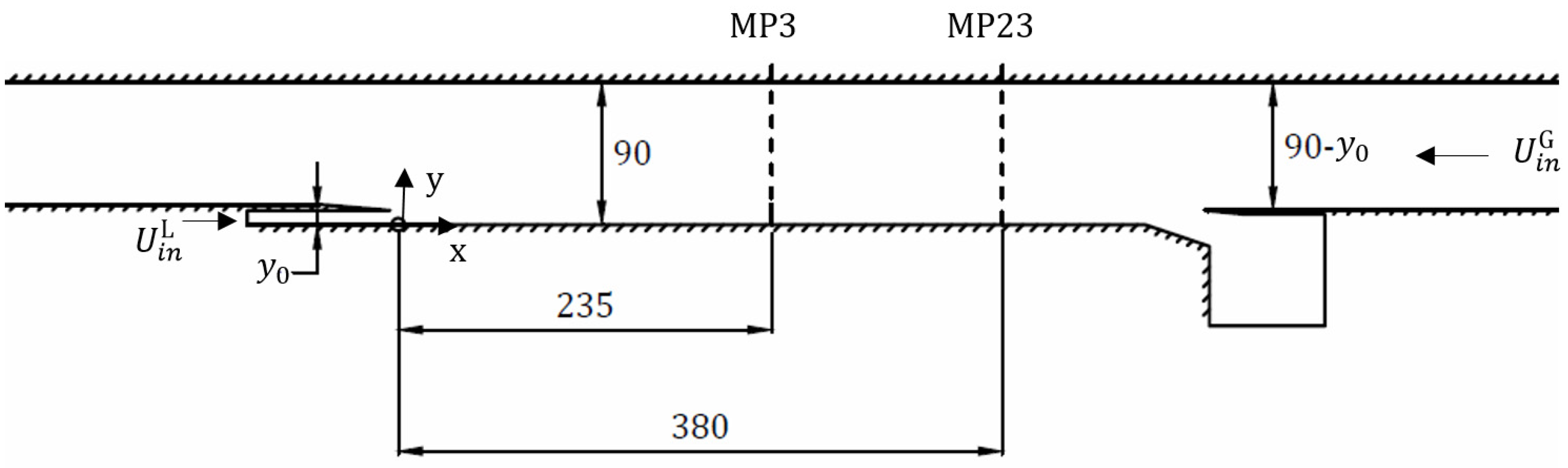
4. Simulation Setup

The experimental validation data used in this work originate from the WENKA facility at KIT [15]—an air–water stratified flow experiment in a horizontal rectangular channel. The structure of the test rig with the corresponding components is shown in Figure 3.

The system consists of two independently controllable water and air circuits. The stratified two-phase flows are directed counter currently in the horizontal measuring section under ambient conditions. Varying the water inlet height $y_0$ and the inlet flow velocities makes it possible to set different flow regimes.

Measurement uncertainties are discussed in [15]. In the discussed experiment, the measurement uncertainty is smaller than 1%.

The calculation area of the WENKA unit used in this paper is shown in Figure 4 in side view. It includes the measuring section with the measuring positions as well as the inlet plates for air and water. An extension of both the air inlet and the air outlet section of about 500 mm is located downstream. The displayed measuring coordinate system is adopted in the simulations, with the y-axis indicating the vertical direction and the x-axis indicating the running length direction. The z-axis as well as the components in the z-direction are neglected in this work because of the quasi 2D-simulations. In the x-direction, there is the measuring section with of approx. 470 mm. The measurement lines from the experiment are marked with MP3 and MP23 and correspond to measurement lines 3 and 23 (Figure 4) from the experiment [15].

The ensemble averaged velocities $\stackrel{=}{{\mathrm{u}}^{\mathrm{k}}}, \stackrel{=}{{\mathrm{v}}^{\mathrm{k}}}$, the square-averaged rates of fluctuation ${\mathrm{u}}_{\mathrm{rms}}^{\mathrm{k}}, {\mathrm{v}}_{\mathrm{rms}}^{\mathrm{k}}$ and the mean Reynolds shear stresses $-\rho \stackrel{=}{\mathrm{u}\prime \mathrm{v}\prime }$ are available for validation at both measurement lines from 2D PIV measurements. The measurement of the phase fraction ${\alpha }^k$with k = G,L in the gas and liquid phase was performed using a resistance probe. With the assumption of isotropic turbulence [15], the turbulent kinetic energy is calculated from:

$$k=\frac{3}{4}\left({\mathrm{u}}_{\mathrm{rms}}^{\mathrm{k}}{}^2+{\mathrm{v}}_{\mathrm{rms}}^{\mathrm{k}}{}^2\right)=\frac{3}{4}\left(\overline{{\mathrm{u}}^k{}^{’2}}+\overline{{\mathrm{v}}^k{}^{’2}}\right)$$

(28)

A detailed description of the boundary conditions in the experiment can be taken from [15], therefore the necessary values are summarized in

Table 7. Boundary conditions from the experiment according to [15].

${\mathit{U}}_{\mathit{i}\mathit{n}}^{\mathit{L}} \left[\mathbf{m}/\mathbf{s}\right]$	${\mathit{U}}_{\mathit{i}\mathit{n}}^{\mathit{G}} \left[\mathbf{m}/\mathbf{s}\right]$	${\mathit{y}}_0 \left[\mathbf{mm}\right]$	$\mathit{R}{\mathit{e}}_{\mathit{d}}^{\mathit{L}}$	$\mathit{R}{\mathit{e}}_{\mathit{d}}^{\mathbf{G}}$	$\mathit{F}{\mathit{r}}_0$
0.7	4.44	9	$1.2\times {10}^4$	$2.7\times {10}^4$	2.36

.

The experimental flow parameters correspond to small-amplitude wavy stratified flow. Consequently, no data for droplet and bubble diameters are available and these model parameters are set to default values of $d_b=d_d=0.001$ m.

Figure 5 shows the block-structured hexahedral grid used in the simulations of the WENKA test rig in an x,y plane. In order to achieve a higher resolution of the turbulent velocity profile at the water inlet, the grid is denser in the y-direction in the range y < $y_0$than in the range y > $y_0$. The cells here are stretched by a factor of 1.3. For the same reason, the grid is locally refined by a factor of two in the y-direction in the area of the water inlet.

The flow was calculated by means of quasi 2D and transient simulations. In

Table 8. Numerical parameters for the simulation.

Simulation Parameters	Selection
Type of analysis	Transient
Total simulation time	$10 \mathrm{s}$
Inital time step	${10}^{-4} \mathrm{s}$
Time step	Adaptive
Time step adjustment	max(CFL) < 1
Maximum time step	1 s
Minimum time step	${10}^{-6} \mathrm{s}$
Advection Scheme	High Resolution
Transient Scheme	Second Order Backward Euler
Time step initialization	Automatic
Turbulence numerics	First Order
Coeff. Loops Number of iterations per time step	1–30
Termination criterion	RMS
residual target	${10}^{-4}$
conservation target	${10}^{-4}$

the numerical parameters of the calculations are summarized. This includes the spatial and temporal discretization parameters as well as the time step procedures in ANSYS CFX.

5. Results

In this section, the results of the simulations performed are presented and validated by the experimental data from [15].

Calculations with the two-fluid model from Section 2 were performed. For the simulation of stratified two-phase flow, the detection of phase boundaries of the different flow morphologies was necessary. For this reason, the AIAD model [7,14,16] with the uniform weighting function from Equation (13) was used.

For all simulations, the calculation area corresponds to the WENKA test rig with the block-structured grid according to Figure. 5. The boundary conditions correspond to the values from Table 7 and Table 8; the velocity profiles were set according to [15].

Figure 6a shows still images from the experiment, illustrating the flow regime in the test section. Figure 6b shows the liquid volume fraction from a simulation with the k-ω turbulence model including the damping term from Equation (23). Figure 6 also shows in Figure 6c the weighting functions f_fs (AIAD 1) and Figure 6d Ψ_surf (AIAD 3) for the detection of the flow regimes in an x,y-section through the measuring section.

Table 9. Mean liquid levels MP3 and MP23

$\mathit{T}\mathit{e}\mathit{s}\mathit{t}.$	Inlet Conditions	$\mathbf{MP}3{\mathit{y}}_{\mathit{m}} \left[\mathbf{mm}\right]$	$\mathbf{MP}23{\mathit{y}}_{\mathit{m}} \left[\mathbf{mm}\right]$
Experiment [15]	─	10.24	11.88
Simulation	Profiles	10.17	11.45

indicates the mean liquid levels $y_{\mathrm{m}}$from the simulation and the measured data for MP3 and MP23.

The table shows that the liquid level $y_{\mathrm{m}}$ obtained in the simulation agrees well with the measured data. With MP3, $y_{\mathrm{m}}$ is slightly overestimated and with MP23 slightly underestimated. All simulations were calculated according to the numerical parameters in Table 8. For the results, the so-called “superficial velocity” is determined and shown here, which is defined by the product of phase fraction and velocity ${\alpha }^G·\mathit{u} .$

5.1. Mesh Sensitivity Study

For simplicity in the following sections, only comparisons of experimental data and numerical results at measurement position MP3 are shown.

To estimate the influence of the mesh on the results, with the guidelines [23] were followed and three different mesh resolutions have been compared. Starting from the coarsest grid, two higher-resolution grids were created by global refinement by a factor of two and four, respectively. These are referred to as “coarse”, “medium” and “fine”. The grid parameters can be found in

Table 10. Mesh parameter.

Mesh	Nodes	$\Delta \mathit{x} \left[\mathbf{mm}\right]$	$\Delta \mathit{y} \left[\mathbf{mm}\right]$	$\Delta \mathit{z} \left[\mathbf{mm}\right]$
coarse	$2.0168\times {10}^4$	7.52	2.22	0.05
medium	$5.94\times {10}^4$	4.46	1.29	0.05
fine	$1.93\times {10}^5$	1.94	0.69	0.05

.

The transient test calculations carried out for the sensitivity study use the resistance formulation at the phase interface ${\mathrm{C}}_{\mathrm{D},\mathrm{fs}}$, which was proposed by Porombka and Hoehne [10]. The k-ω turbulence model with damping term according to Equation (23) is also used in connection with the subgrid wave turbulence “SWT” according to [4]. The results for all mesh resolutions are listed in

Table 11. Standard deviations of the velocities${\mathrm{u}}^G {\mathrm{und} \mathrm{u}}^L$ for the Mesh sensitivity study.

Mesh	$\mathit{\sigma } \left({\mathbf{u}}^{\mathit{G}}\right)$	$\mathit{\sigma } \left({\mathbf{u}}^{\mathit{L}}\right)$
Coarse	0.538%	0.6357%
Medium	0.0158%	0.0114%
Fine	0.0035%	0.0047%

. The standard deviations $\sigma \left({\mathrm{u}}^k\right)$were determined at a monitor point with MP3 within the respective phase.

It can be clearly seen that the smallest fluctuations in speed ${\mathrm{u}}^k$ result with the finest mesh. The results of the calculations are shown in Figure 7. The obtained profiles of the horizontal and vertical components of the velocities ${\mathrm{u}}^k$ and ${\mathrm{v}}^k$ as well as the gas phase component ${\mathsf{\alpha }}^G$ for MP3 for the three different meshes “coarse”, “medium” and “fine” are considered in the following. The calculations were performed with the uniform weighting functions (AIAD 3) and are compared to the measured values (Exp) according to [15].

From the results it can be observed that $u^{\mathrm{G}}, u^{\mathrm{L}}$and ${\alpha }^{\mathrm{G}}$ for all three meshes at MP3 are close to the measured values (Figure 8). Here emerges a dominant influence of the weighting functions of the AIAD 3.

On the other hand, it can be seen in Figure 7b that the profile of ${\mathrm{v}}^{\mathrm{G}}$ shows no physical fluctuation for all three grids.

With ${\mathrm{v}}^{\mathrm{L}}$ a good agreement with the measured values can be achieved for all meshes on the duct wall at $y=0 \mathrm{mm}$. However, the divergences increase near the phase boundary at $y_m$, as shown in Figure 9b. This could be due to the inlet conditions from Section 4 or a greater degree of turbulence at the water inlet in the experiment.

In summary, the results of the fine, medium and coarse meshes show no qualitative approximation to the measured profiles with increasing mesh resolution.

All calculations in this work were carried out with the medium mesh according to the mesh parameters from Table 11.

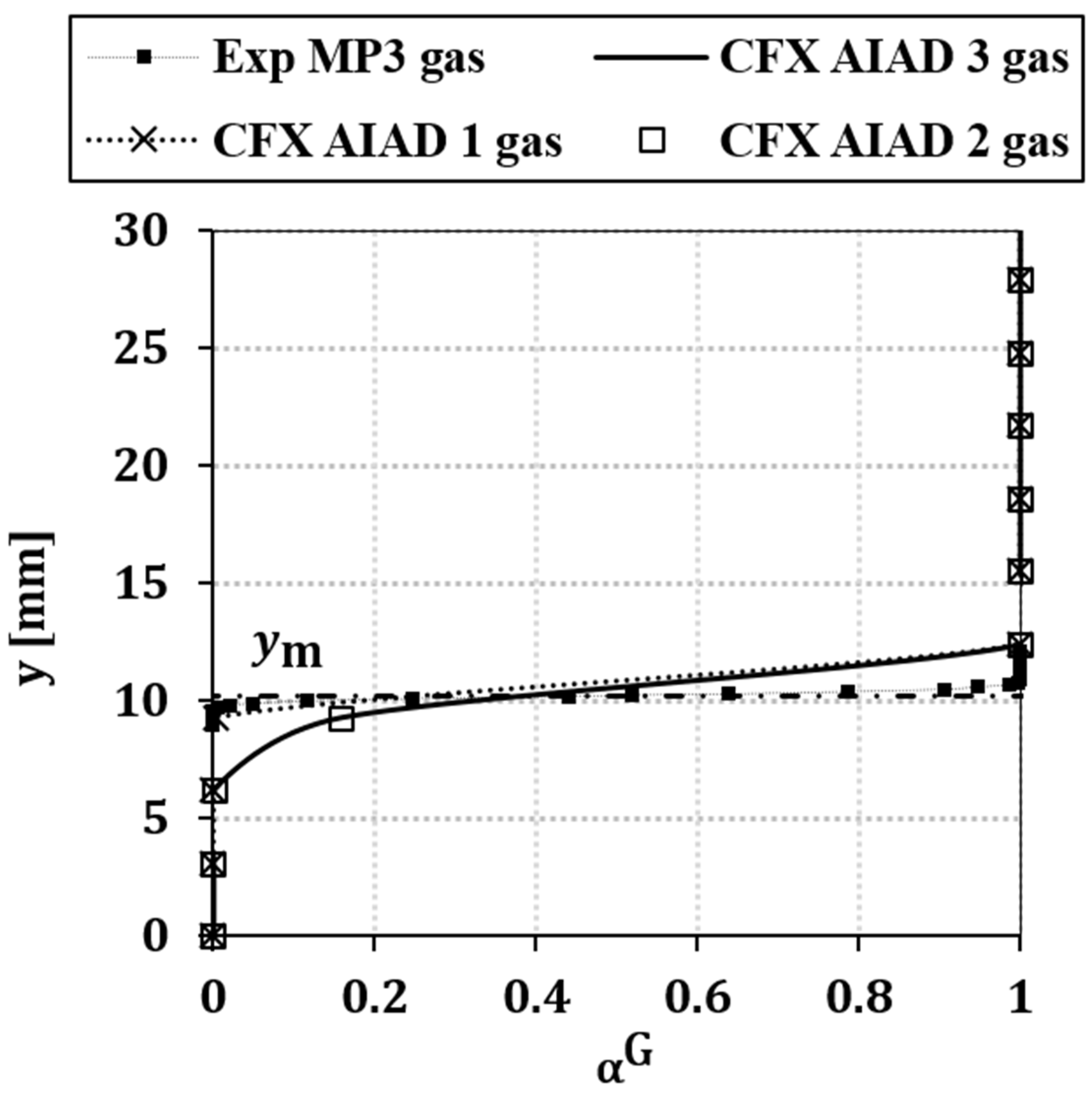
5.2. Influence of Weighting Functions

Three comparative calculations were performed to validate the uniform weighting functions in the AIAD model. The first contained the weighting functions 1 in the AIAD model according to [14], which is referred to as “AIAD 1”. The second one contained the weighting functions 2 also in the AIAD model according to [12], which is designated “AIAD 2” and a third calculation with the current uniform weighting functions according to [8], which is designated “AIAD 3”.

All transient calculations here use the two-fluid model and the drag formulation at the phase interface ${\mathrm{C}}_{\mathrm{D},\mathrm{fs}}$according to [6]. The turbulence model is, in all cases, the k-ω model with the damping term from Equation (23) and is used in connection with the subgrid wave turbulence according to [4]. The boundary conditions are selected according to Table 7 and the simulations use the grid parameters from Table 11 and the numerical parameters from Table 8.

The mean liquid level $y_{\mathrm{m}}$does not change for MP3 and MP23 for the three simulations. It remains stable compared to the data shown in Table 10.

To validate the uniform weighting functions, the following figures show the profiles of the horizontal and vertical components of the velocities ${\mathrm{u}}^k {\mathrm{and} \mathrm{v}}^{\mathrm{k}}$as well as the turbulent kinetic energy $k^{\mathrm{k}}$of the two phases and the gas phase fraction ${\alpha }^G$for MP3 for the three different weighting functions “AIAD 1”, “AIAD 2” and “AIAD 3” respectively. These can be seen in comparison to the measured values according to [15] “Exp” (Figure 10, Figure 11, Figure 12 and Figure 13).

In general, the results of “AIAD 2” and “AIAD 3” show good agreement for all parameters investigated for both the gas and liquid phases. Most of the deviations with respect to “AIAD 1” are particularly noticeable here near the phase boundary at y_m.

In the profiles of ${\mathrm{u}}^G$,${\mathrm{u}}^L, k^G \mathrm{and} k^L$for the three weighting functions in both measuring points, a similar course can be observed to the measured values in the regions near the channel wall at y = 0 mm and y = 90 mm respectively.

The profiles of the vertical velocity component ${\mathrm{v}}^G$for the three weighting functions for MP3 do not show good agreement with respect to the measured values. In Figure 10b and Figure 11b a non-physical spatial variation can be seen in “AIAD 1” which differs from the other weighting functions.

The profile of the gas phase fraction ${\alpha }^G$in both measuring points shows a good agreement for the three different weighting functions and an asymptotic approximation to the measured values at $y_{\mathrm{m}}$.

In conclusion, the results show no significant differences, as can be seen in the simulations of the weighting functions of the AIAD model “AIAD 2” and “AIAD 3” for the respective parameters.

5.3. Influence of Turbulence Modeling

For the evaluation of the effect of the turbulence modeling at the phase boundary interface of the flows in connection with the uniform weighting functions of the AIAD model, two comparative calculations were carried out with the two-equation turbulence models from Section 3. The transient calculations use the k-ω and k-ε turbulence models with a damping term according to Equation (27). The simulations of both turbulence models are performed with the resistance formulation at the phase boundary interface ${\mathrm{C}}_{\mathrm{D},\mathrm{fs}}$ according to [6].

Furthermore, the configuration of the calculations corresponds essentially to the description in Section 4.

The following figures show the parameters ${\mathrm{u}}^k{, \mathrm{v}}^k, k^k, {\alpha }^G$and the modeled Reynolds shear stress ${\tau }_{\mathrm{T},ij}^{\mathrm{k}}$at the MP 3 for the validation of the turbulence modeling. The simulations show the results with the k-ω model “AIAD 3 k-o” and with the k-ε model “AIAD 3 k-e” and they are set up with the measured values “Exp” and the standard profiles of the k-ω model without turbulence damping “Standard” according to [6] (Figure 14, Figure 15, Figure 16, Figure 17 and Figure 18).

The comparison with the measured data shows a large deviation of the liquid level for the k-ω without damping function (

Table 12. Averaged liquid level at MP3 and MP23.

$\mathit{T}\mathit{e}\mathit{s}\mathit{t}.$	$\mathbf{MP}3{\mathit{y}}_{\mathit{m}} \left[\mathbf{mm}\right]$	$\mathbf{MP}23{\mathit{y}}_{\mathit{m}} \left[\mathbf{mm}\right]$
Measurements	10.24	11.88
k-ω with damping	10.17	11.45
k-ε with damping	10.14	11.39
k-ω without damping	23.52	18.68

). This is due to a flow regime deviating from the experiment. The liquid level of k-ω and k-ε models with turbulence damping corresponds to the measured data.

In comparison to the measured values as well as to the results of the standard k-ω model without turbulence damping, a clear influence of the turbulence damping can be seen in most cases.

The results of ${\mathrm{u}}^G$,${\mathrm{u}}^L \mathrm{and} {\alpha }^G$ (Figure 14 and Figure 15,18) show no significant divergence between the k-ω and k-ε models with turbulence damping and a good agreement with the measured values. A good agreement of the profile of ${\mathrm{v}}^G$with the measured values is shown in Figure 14b. In contrast, the profile of ${\mathrm{v}}^L$in Figure 15b shows a non-physical local variation.

In Figure 16 a,b the turbulent kinetic energy is shown. This shows a slight improvement in the convergence of $k^G$ with the measured values for the k-ε model with turbulence damping near the phase boundary. In addition, the profiles with “Standard” were scaled by a factor of 1/10 at both measuring points, since the profile of$k^G$ differs from the measured values by more than one order of magnitude.

When using the k-ε model with turbulence damping in relation to the k-ω model with turbulence damping, the following can be seen here:

The Reynolds shear stresses are shown in Figure 17. The results are determined using the modelled eddy viscosity ${\mu }_{T,ij}^k$in Equation (19) for each phase. The evaluation of the Reynolds shear stresses in view Figure 17a shows a slight convergence in both measurement points with the measured values for the k-ω model with turbulence damping. In view Figure 17b, the simulation results of both turbulence models with damping term show a non-physical local variation of the Reynolds shear stresses at MP3. The reason for this could not be clearly determined. In addition the gas phase fraction at MP3 for the investigated turbulence models is shown in Figure 18.

The results of the calculations show a dominant influence of the turbulence damping at the phase boundary of the present flow regime. The use of the k-ε model with damping term ${\mathrm{S}}_{\mathrm{D}}^{\mathrm{k}}$provides a special convergence behaviour at some turbulence parameters such as $k^G$and${\mathrm{v}}^G$ compared to the k-ω model with turbulence damping.

6. Summary and Conclusions

The objective of the present work was the validation of the new uniform weighting functions in the AIAD model according to [8] for the modeling of horizontal two-phase flows with phase interfaces in the two-fluid model. For the simulation of stratified two-phase flows with different flow regimes, the detection of phase boundaries of the different flow morphologies is required. For this reason, the AIAD model according to [3,5,13] was used in this work with a new approach for the formulation of the weighting functions.

The implementation of the new uniform weighting functions was suitable for the description of the momentum exchange at the phase boundary in the AIAD model, and further in turbulence modelling on two-phase flows with phase boundaries.

The validation of the simulations was carried out with experimental data from a suitable test case, whose geometric boundary conditions and broad database were available.

In the first part of the work, some relevant publications on the topic of horizontal two-phase flows were presented and subsequently the mathematical principles of the two-fluid model used and the AIAD model were described in Section 2. Additionally, the description of the approach for modelling the momentum exchange at the phase boundary interface in the AIAD model was dealt in this section, where the drag modelling for different flow regimes was analyzed and the new approach for the drag coefficient at the phase boundary was evaluated from the consideration of the shear stresses at the phase boundary.

In Section 3, the turbulence modeling of horizontal two-phase flows with phase interfaces was dealt with. In particular, the adaptation of the k-ω turbulence model by means of a damping term was described in the ω transport equation. The ω transport equation was transferred to the formulation for ε transport equation in order to be able to use a modified k-ε turbulence model.

The WENKA test facility was selected to simulate a suitable test case. The configuration of the test facility and the execution of the experiment were described in Section 4. It is an air–water circulation channel with a rectangular cross-section of the test section for the investigation of horizontal, stratified and opposing two-phase flows. By means of PIV measurements and ensemble averaging, the time-resolved velocity fields were recorded. The measurement of the phase fraction in both phases was performed by a resistance probe.

In previous work, the flow regime was not correctly reproduced from the experiment with a simple homogeneous modeling of the two-phase flow.

The results of the validation calculations were shown and discussed in Section 5. The simulations with the uniform weighting functions in the AIAD model resulted in an improvement for the detection of the phase boundary.

In the comparative calculations with the turbulence models, a dominant influence of the turbulence modeling on the two-phase flow was found. When using the k-ω turbulence model without damping, flow regimes deviated from those of the experiment. Parameters such as the turbulent kinetic energy were overestimated by more than one order of magnitude in these cases.

By using a damping term according to [4] in the ω transport equation, the measured turbulence parameters could be reproduced much better by the k-ω and k-ε turbulence models.

In addition, the adaptation of the model constants of the weighting functions could better reflect the phase boundary even with sharp jumps of the phase fraction. In subsequent simulations, the results should be compared with various other experimental data.