Curated Dataset for Red Blood Cell Tracking from Video Sequences of Flow in Microfluidic Devices

Abstract

This work presents a dataset comprising images, annotations, and velocity fields for benchmarking cell detection and cell tracking algorithms. The dataset includes two video sequences captured during laboratory experiments, showcasing the flow of red blood cells (RBC) in microfluidic channels. From the first video 300 frames and from the second video 150 frames are annotated with bounding boxes around the cells, as well as tracks depicting the movement of individual cells throughout the video. The dataset encompasses approximately 20,000 bounding boxes and 350 tracks. Additionally, computational fluid dynamics simulations were utilized to generate 2D velocity fields representing the flow within the channels. These velocity fields are included in the dataset. The velocity field has been employed to improve cell tracking by predicting the positions of cells across frames. The paper also provides a comprehensive discussion on the utilization of the flow matrix in the tracking steps.

1. Introduction

Scientists need information on the structure and behavior of individual cells for various tasks, such as creating models, validating experiments, and making predictions. Previously, data was obtained through bulk measurements, but advances in technology have made single-cell analysis possible through methods such as single-cell sequencing, improved imaging, and microfluidics. High-throughput single-cell analysis offers both accuracy and large amounts of data, but analyzing this data, especially image segmentation and cell tracking, remains mostly a manual and time-consuming process.

Algorithms that automate the detection and tracking of cells with minimal human intervention would greatly increase the productivity of biologists and the availability of data. Cell tracking [1] provides information on cell behavior, cell lineage, and cell morphology [2], and can help investigate correlations between diseases and abnormal cell behavior [3]. Cell tracking involves accurately segmenting cell boundaries, tracking cell movements over time, determining cell velocity and trajectory, and detecting changes in cell lineage due to cell division or death. However, this task is complicated due to low-resolution images, small cell size, similarity of cells, and the fact that cells are in reality 3D but are only captured in 2D. Existing cell tracking algorithms can be divided into two groups: contour matching methods [4,5] and cell detection and tracking methods [6,7]. The latter group is the focus of this discussion.

In this work, we provide a dataset that can be used for benchmarking the cell detection and cell tracking algorithms. Details about the dataset availability are given in Supplementary Materials section. The dataset contains two video sequences of a laboratory experiment recording the flow of red blood cells (RBC) in microfluidic channels. Part of the image sequence is annotated with bounding boxes around the cells and with the definition of tracks of individual cells across the video sequence. The dataset contains around 20,000 bounding boxes and 350 tracks. Furthermore, we present a broader discussion about using the flow matrix in the tracking of steps. A flow matrix is a vector field that gives the velocity profile of the fluid flow in which the cells are immersed, and as such it could give significant information about how the cells propagate from frame to frame.

1.1. Cell Detection

The cell tracking problem can be divided into two parts: cell detection and cell tracking. Cell detection, the first part, is well understood and has been solved by various methods. Among traditional methods (i.e., those that do not use the methods of deep learning), the so called Hough transform has been successively used to detect the cell centers [8,9]. Another example is the level set method, where the boundary of a cell is represented by a zero-level set of 3D functions and the evolution of such contours is tracked [10]. Traditional methods also use different strategies to enhance the results, for instance, finding uniform areas, boundaries, or identifying bright spots and maxima at low resolution [11]. To segment the cell boundaries, image features are computed such as simple pixel or voxel intensities, their local averages, or more complex local image descriptors of shapes or textures. These features are then utilized using different principles such as thresholding [3] and edge detection [12]. For a recent comprehensive overview of other traditional methods for cell detection we refer to [13].

Deep machine learning is quite common in computer vision. Convolutional neural networks (CNN) outperform a lot of traditional methods in different tasks, for example, image classification [14], object recognition [15], detection, segmentation, and region extrapolation [16]. Object detection makes use of convolutions to effectively capture crucial features in images. Therefore, making use of existing CNN frameworks is valuable because it has the potential to boost the base performance of these techniques in the near future.

This work presents a dataset consisting of annotated frames of two video sequences. This dataset has been used in [17], where the author implemented a conventional image processing algorithm for the first video in the dataset, detecting the centers of the cells. The algorithm sequentially applied a background subtraction method, canny edge detection, a Hough transform, and thresholding. The Hough transform created dense clusters of high-intensity points, where centers of shapes are located; see Figure 1. This algorithm, however, required expert input to tune the parameters and did not achieve sufficient results.

To avoid the need for expert input for parameter tuning, convolutional neural networks have been used to detect the cells. In [18], a thorough analysis of the performance of three CNN architectures on the problem of cell detection was presented: Faster RCNN [16], R-FCN [19], and SSD [20]. Faster RCNN and R-FCN provided similar results, whereas SSD performed worse than the other architectures. These frameworks were tested on a dataset comprised of 200 frames of the first video from the dataset, which amounted to about 8000 positives RBC samples and about 80,000 negative background samples. The best results were obtained using the Faster RCNN framework, which provided 98.3% precision and 88.8% recall.

1.2. Cell Tracking

Conventional cell tracking algorithms depend on the outcome of the cell detection process. To link the detected cells across multiple frames into trajectories, these algorithms typically employ probabilistic methods to establish temporal relationships between the segmented cells [7,21]. This can be achieved by either using a two-frame or multiframe sliding window, or even for all frames at once.

With the advent of deep machine learning has come great advances in visual object tracking [22]. However, tracking cells with visual tracking methods such as Siamese tracers [23] is very challenging. This difficulty is mainly due to the high density of blood cells in a 3D environment as well as their high visual similarity. Therefore, the utilization of CNN in the cell tracking step is not as widespread. Most cell tracking algorithms that employ deep learning do make use of CNN in the first step of the process, which is cell detection. In cell linking algorithms they use, for example, a min-cost flow solver [24]. The number of works that use CNN in the tracking step is limited. In [25], the authors use CNN to predict cell distance maps and novel neighbor distance maps that are subsequently used as input for a watershed post-processing. In [26], the author designed a CNN that combines kernelized correlation filters for tracking. Although the idea is sound, the reported results are mediocre. This line was not pursued further. In [27], the authors propose a cell tracking method composed of, first, the particle filter model to produce a set of candidate bounding boxes, then, second, a trained observation model provides the confidence probabilities corresponding to all of the candidates and selects the candidate with the highest probability as the final prediction. Finally, a multi-task observation model is use for the variation of the tracked cell over the entire tracking procedure. This procedure considers single-cell tracking and does not solve multi-object tracking.

In recent work [28], the authors devised a deep learning method and published a dataset for benchmarking of the cell tracking algorithms. This dataset however contains very low velocity motions of the cells. A similar attempt was made in [29], where the authors employed an innovative approach of machine learning to perform cell tracking and lineage reconstruction. The dataset used in this work contains time-lapse movies of Escherichia coli cells trapped in a microfluidic device for long-term single-cell analysis. The cells move very little during these time-lapse movies which makes high fidelity results possible.

Tracking of cells in a micro-flow within microfluidic devices is a specific task. The cells are generally moving with high velocities, their shape can change, and the direction and velocity of flow changes as well. These flow properties are particularly challenging and have not been tackled by CNNs at either the detection or tracking level. The dataset presented in this work has been used for conventional cell tracking [17,18]. Conventional cell tracking algorithms rely on linking positions of cells from one frame to another using geometrical and physical information including the current cell velocity. The direction of a cell is influenced by two factors. The first factor is the previous history of a cell, i.e., its velocity over time, and the second factor is the behavior of the fluid. While the former is fairly trivial to compute from previous tracked bounding boxes, the latter can heavily change the predicted new position.

In [17,18], the conventional cell linking algorithm was performed in three steps.

• First simple pass-through The task of this method is to create initial tracks on the basis of a simple condition: If detected cells are in two consecutive frames and they are closer than a given threshold r, they are linked to one track. Another criterion for the connection is that there is exactly one cell in the next frame within distance r.
• Flow matrix creation The flow matrix of an image stores the velocity profile that can be used for identification of the cell’s next frame position. The idea behind the use of a flow matrix is that the channel in which the cells are flowing is fixed and therefore the movement of a cell can be approximated by the movement of cells that passed through the same location before or by the movement of the fluid.
• Second complex pass-through After the first pass-through, there can be many gaps in tracks between the previous frame and the next frame which will cause fragmentation of the tracks. The second pass-through serves to bridge the possible gaps. Dealing with gaps in detection is pretty straightforward, one can estimate the future position of a cell by computing its proposed position from the flow matrix in the first missing gap, and then the next missing gap, up to the gap maximum.

The results of this algorithm, presented in [18], show that the detected tracks are significantly shorter than the true tracks. The average length of the true tracks in the first video is 139 frames, while the above conventional algorithm gives an average length of 59 frames. This determines the fragmentation of the true tracks to be 2.3 fragments per track on average.

2. Dataset

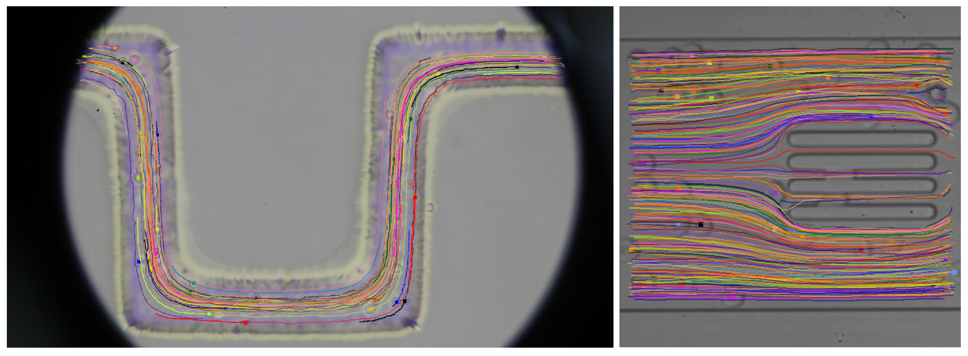
The dataset contains two videos. The first video contains a recording of the flow of a cell suspension in a U-shaped channel, the direction of the flow is from right to left; see Figure 2, left. Cells near the channel borders move slowly and cells in the channel center may move faster, depending on how deep they are suspended. Detailed pictures of several cells are shown in Figure 3. The second video shows the flow of a cell suspension in a channel that is constricted by four horizontal obstacles creating three narrow slits with different widths; see Figure 2, right. Cells travel from left to right. Some cells enter the constrictions and, highly deformed, they travel through the constriction. Some cells avoid the constrictions. For clarity, we define the Cartesian axes $x,y,z$ such that both videos depict the $xy$ plane. When referring to depth, we mean the dimension in the z-axis.

2.1. U-Shaped Channel

The rectangle depicted in the video frames has physical dimensions of $400\mathsf{\mu }\mathrm{m}$ width and $225\mathsf{\mu }\mathrm{m}$ height. The frame resolution is $1280\times 720\mathrm{px}$, which gives the transformation $1\mathrm{px}=3.2\mathsf{\mu }\mathrm{m}$. The physical dimensions of the channel are 32 $\mathsf{\mu }\mathrm{m}$ width and approximately 156 $\mathsf{\mu }\mathrm{m}$, the length of one side of the U-shape. The depth of the channel is $32\mathsf{\mu }\mathrm{m}$ and the cross-section is thus a square. The optics of the microscope is focused to the middle of the channel depth which results in blurred cells that flow above or beneath the plane of focus. The laws of fluid dynamics state that the fluid (and thus the cells as well) has the highest velocity in the middle of the channel’s cross-section. Therefore, the cells appearing at the channel walls have low velocity. Cells that appear in the middle of the channel may flow in different fluid depths and thus may have different velocities. Those having a z-coordinate close to $16\mathsf{\mu }\mathrm{m}$ travel fast, while those with a z-coordinate close to 0 or $32\mathsf{\mu }\mathrm{m}$ travel slowly. This results in possible overlapping of the cells as depicted in Figure 3, on the left.

The maximal velocity of the fluid will be achieved in the middle of the channel. Since cells flow freely with no obstacles, the maximal fluid velocity may be determined from the maximal velocities of the flowing cells. Considering the $20\mathrm{fps}$ frame rate in the video and the maximal distance between the cells in consecutive frames, we can determine the maximal velocity in the channel to be around $11\mathrm{px}/frame=11\times 20/3.2=68.75\mathsf{\mu }\mathrm{m}/\mathrm{s}$.

2.2. Channel with Slits

The rectangle depicted on the video frames has dimensions of $107.8\times 107.8\mathsf{\mu }\mathrm{m}$. The frame resolution is $512\mathrm{px}$, which gives the resolution $4.75\mathrm{px}=1\mathsf{\mu }\mathrm{m}$. The physical dimensions of the channel are $107.8\mathsf{\mu }\mathrm{m}\times 85\mathsf{\mu }\mathrm{m}.$ The depth of the channel is only $6\mathsf{\mu }\mathrm{m}$ and the cells are thus forced to have their main plane semi-parallel to the $xy$-plane. In the channel there are four obstacles forming three slits with different widths of $2.52\mathsf{\mu }\mathrm{m},3.16\mathsf{\mu }\mathrm{m}$, and $3.79\mathsf{\mu }\mathrm{m}$. Here, the maximal velocity of the fluid will be reached in the slits but only when the slits are not occupied with cells. Therefore, the maximal velocity of the fluid will not coincide with the maximal velocities of the cells. In the wide portions of the channel, cell velocities coincide with the average velocity of the fluid. Typical values are 20 to $30\mathrm{px}/frame$. Considering the $29.87\mathrm{fps}$ frame rate in the video and the maximal distance between the cells in consecutive frames, we have typical velocities of cells in wide portions of the channel of around $20\mathrm{px}/frame=20\times 29.87/4.75=125\mathsf{\mu }\mathrm{m}/\mathrm{s}$ to $188\mathsf{\mu }\mathrm{m}/\mathrm{s}.$

2.3. Annotated Images

The dataset contains annotations of bounding boxes around the cells and information about the cell tracks; see Figure 2 and Figure 4. The first video has a resolution of $1280\times 720\mathrm{px}$, with about 50 RBCs per frame on average and the RBCs are $25\mathrm{px}$ to $35\mathrm{px}$ in size on average. The second video has a $512\times 512\mathrm{px}$ resolution, has about 35 RBCs per frame on average, and the RBCs are $45\mathrm{px}$ to $55\mathrm{px}$ in size on average. More detailed information about the dataset videos is given in

Table 1. Comparison of the two datasets. Note that cell sizes are different and tracks are also fundamentally shorter.

	Total	Annotated	Bounding	Tracks	Average	Average	Average	Track IDs
	Frames	Frames	Boxes		Cell Width (px)	Cell Height (px)	Track Length	with Still Cells
U-shaped channel	2992	300	15,137	84	25.0	24.4	180.2	7, 20, 35, 41
Channel with slits	239	150	5730	268	39.2	38.9	21.4	267

.

The tracking part of our dataset is composed of bounding boxes connected into tracks. Both our videos are annotated, the first containing tracks with 176.9 frames on average and the second containing tracks with 18.8 frames on average. Both videos demonstrate completely different behavior of the cells and model the required task well.

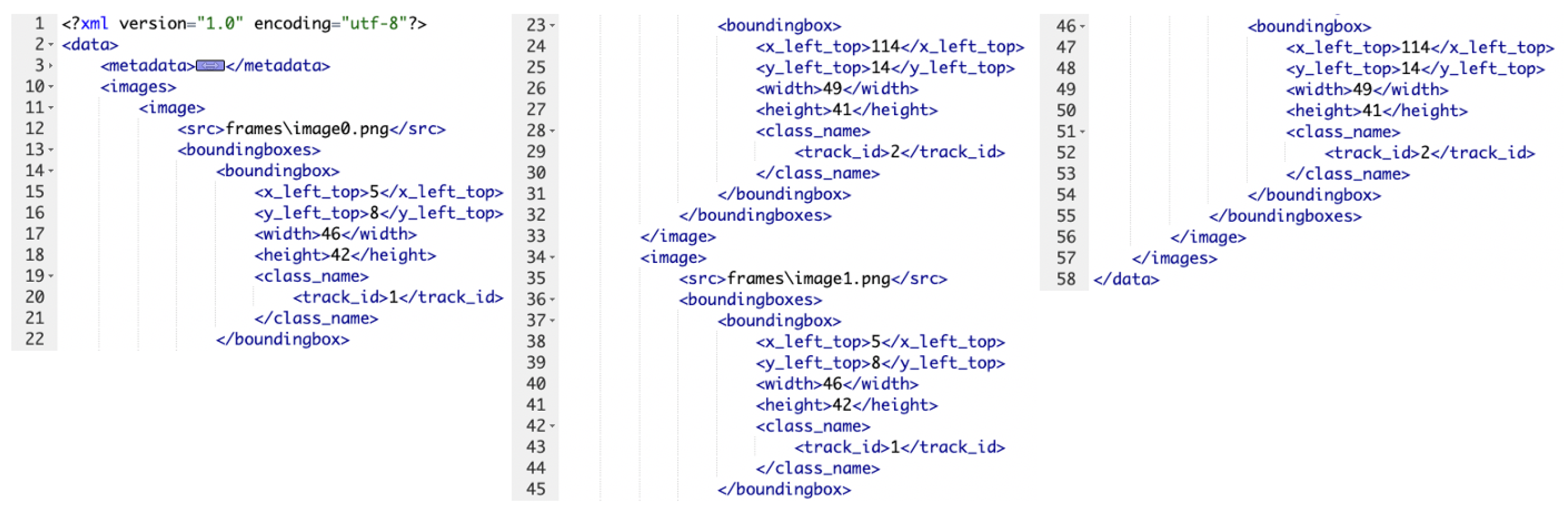
The annotations (bounding boxes and tracks) are stored in one XML file per video. Root element data contains two elements metadata (with some general information) and images. Element images contains as many elements image as there are frames in the video. Each element image contains two elements: src (containing the relative path to the image file) and boundingboxes (having as many elements boundingbox as there are annotated cells in that particular image frame). Element boundingbox carries information about the coordinates of the upper left corner of the bounding box and its width and height (x_left_top, y_left_top, width, height). Additionally, it has element class_name, which holds the identification of the track (track_id) which that particular cell belongs to. An example of an XML file for a toy-video containing only two frames from Figure 5 is depicted in Figure 6.

Annotations of bounding boxes and the tracks were obtained using in-house annotation software, version number 1.4.1.

2.4. Flow Matrices

Flow matrices contain information about the fluid flow in the channels. In the dataset, we provide data obtained from the CFD simulation using the PyOIF package version pyoif-v2.1 [30] of the ESPResSo [31] scientific software, available at [32]. PyOIF is capable of modeling a flow of a fluid in microfluidic channels with complex geometries and has been used in numerous computational works [33,34,35,36]. We set up two simulations, one for each video, with specific channel geometries as described above in Section 2.1 and Section 2.2. The inlet conditions were set so that they corresponded to the maximal flow velocity in the U-channel and to the typical flow velocity in the wide sections of the channel with slits.

The CFD simulation is a full 3D simulation with a 3D velocity field. However, the flow in the z-axis is laminar and all velocity vectors have a negligible z-component. Therefore, it is sufficient to provide a 2D velocity field defined on an $xy$-cross-section of the simulation box. We decided to cut the simulation box by a plane parallel to the $xy$-plane in the middle of the z-dimension where the fluid velocity is maximal. Illustrative figures of flow matrices are depicted in Figure 7. A flow matrix, as a 2D vector field, is given by providing information about the datapoints. One datapoint contains the x- and y-coordinates of a pixel and the corresponding velocity vector $(u,v)$. Data for both flow matrices are given in a csv file containing four rows of comma separated values. The first and second rows contain the x- and y-coordinates of all the datapoints. The third and fourth row contain values for the x- and y-coordinates of the corresponding velocity vector. Such a format can be easily visualized by, e.g., MATLAB or Python.

3. Discussion

This dataset contains annotations of flowing cells, so even if a cell is a bit damaged but travels through the channel, the dataset does contain its bounding boxes and track ID. Further, if a cell is physically under or above the microscope’s focus depth (so the cell is blurred, but still visible), the dataset still contains its annotations. Some cells become invisible on several frames during their travel through the channel. This is due to the cells sinking out of focus completely so that they are undetectable on individual frames. Or, they may be hidden behind other cells. On these frames, such cells are not annotated, however, as soon as the cells reappear, they receive the same track ID as before. This is useful when an algorithm attempts to fill in the gaps in tracks. There are several still cells in the videos that are not moving, for example, because they are attached to the channel surface. The dataset contains bounding boxes of such cells, and a track ID is assigned to them, namely, in the U-shaped channel we have four still cells with track IDs 7, 20, 35, and 41. In the channel with slits, we have only one still cell, with the track ID 267. We also included cells that are located at the edge of the frame and are not displayed as a whole, but only in part. We believe that this might be useful for testing of incomplete cell detection. In case the users of the dataset do not wish to include such cells, they can easily filter them out using the distance of BBOX from the edge of the frame.

4. Conclusions

The provided dataset has been used in several studies for the development of conventional cell detection and cell tracking algorithms [37], for comparison of different neural network approaches for cell detection [18], and for linking of segmented tracks using neural networks [38]. The dataset can be used for benchmarking any cell tracking or cell detection algorithms, such as those presented in [39,40]. A unique feature of the provided dataset is that it contains a flow matrix. This enables new approaches to cell tracking that use fluid flow information in conjunction with image information. In addition, the dataset can also be used to validate fluid flow estimation from image data or to solve sub-tasks such as cell movement prediction. The availability of the whole video files makes it possible to extend the dataset with annotations of further frames.

References

- Huh, S.; Eom, S.; Bise, R.; Yin, Z.; Kanade, T. Mitosis detection for stem cell tracking in phase-contrast microscopy images. In Proceedings of the 2011 IEEE International Symposium on Biomedical Imaging: From Nano to Macro, Chicago, IL, USA, 30 March–2 April 2011; pp. 2121–2127. [Google Scholar]
- Yang, F.; Mackey, M.A.; Ianzini, F.; Gallardo, G.; Sonka, M. Cell Segmentation, Tracking, and Mitosis Detection Using Temporal Context. In Proceedings of the Medical Image Computing and Computer-Assisted Intervention–MICCAI 2005, Palm Springs, CA, USA, 26–29 October 2005; Duncan, J.S., Gerig, G., Eds.; Springer: Berlin/Heidelberg, Germany, 2005; pp. 302–309. [Google Scholar]
- Chen, X.; Zhou, X.; Wong, S. Automated segmentation, classification, and tracking of cancer cell nuclei in time-lapse microscopy. IEEE Trans. Biomed. Eng. 2006, 53, 762–766. [Google Scholar] [CrossRef]
- Dufour, A.; Thibeaux, R.; Labruyère, E.; Guillen, N.; Olivo-Marin, J. 3-D Active Meshes: Fast Discrete Deformable Models for Cell Tracking in 3-D Time-Lapse Microscopy. Image Process. IEEE Trans. 2011, 20, 1925–1937. [Google Scholar] [CrossRef]
- Ka, M.; K, O.; Garasa, S.; Rouzaut, A.; Muñoz-Barrutia, A.; Ortiz-de Solorzano, C. Segmentation and Shape Tracking of Whole Fluorescent Cells Based on the Chan-Vese Model. IEEE Trans. Med. Imaging 2013, 32, 995–1006. [Google Scholar] [CrossRef]
- Turetken, E.; Wang, X.; Becker, C.; Haubold, C.; Fua, P. Network Flow Integer Programming to Track Elliptical Cells in Time-Lapse Sequences. IEEE Trans. Med. Imaging 2016, 36, 942–951. [Google Scholar] [CrossRef] [PubMed] [Green Version]
- Schiegg, M.; Hanslovsky, P.; Haubold, C.; Koethe, U.; Hufnagel, L.; Hamprecht, F.A. Graphical model for joint segmentation and tracking of multiple dividing cells. Bioinformatics 2014, 31, 948–956. [Google Scholar] [CrossRef] [PubMed] [Green Version]
- Illingworth, J.; Kittler, J. The Adaptive Hough Transform. IEEE Trans. Pattern Anal. Mach. Intell. 1987, PAMI-9, 690–698. [Google Scholar] [CrossRef] [PubMed]
- Yuen, H.K.; Illingworth, J.; Kittler, J. Ellipse Detection using the Hough Transform. In Proceedings of the AVC, Manchester, UK, 31 August–2 September 1988; pp. 41.1–41.8. [Google Scholar] [CrossRef] [Green Version]
- Lin, G.; Adiga, U.; Olson, K.; Guzowski, J.F.; Barnes, C.A.; Roysam, B. A hybrid 3D watershed algorithm incorporating gradient cues and object models for automatic segmentation of nuclei in confocal image stacks. Cytom. Part A 2003, 56, 23–36. [Google Scholar] [CrossRef]
- Wuttisarnwattana, P.; Gargesha, M.; van’t Hof, W.; Cooke, K.R.; Wilson, D.L. Automatic Stem Cell Detection in Microscopic Whole Mouse Cryo-Imaging. IEEE Trans. Med. Imaging 2016, 35, 819–829. [Google Scholar] [CrossRef] [Green Version]
- Wahlby, C.; Sintorn, I.M.; Erlandsson, F.; Borgefors, G.; Bengtsson, E. Combining intensity, edge and shape information for 2D and 3D segmentation of cell nuclei in tissue sections. J. Microsc. 2004, 215, 67–76. [Google Scholar] [CrossRef]
- Thomas, R.M.; John, J. A review on cell detection and segmentation in microscopic images. In Proceedings of the 2017 International Conference on Circuit, Power and Computing Technologies (ICCPCT), Kanyakumari, India, 20–21 April 2017; pp. 1–5. [Google Scholar]
- Krizhevsky, A.; Sutskever, I.; Hinton, G.E. ImageNet Classification with Deep Convolutional Neural Networks. Commun. ACM 2017, 60, 84–90. [Google Scholar] [CrossRef] [Green Version]
- Donahue, J.; Jia, Y.; Vinyals, O.; Hoffman, J.; Zhang, N.; Tzeng, E.; Darrell, T. DeCAF: A Deep Convolutional Activation Feature for Generic Visual Recognition. In Proceedings of the 31st International Conference on Machine Learning, Beijing, China, 21–26 June 2014; Xing, E.P., Jebara, T., Eds.; PMLR: Bejing, China, 2014; Volume 32, pp. 647–655. [Google Scholar]
- Ren, S.; He, K.; Girshick, R.; Sun, J. Faster r-cnn: Towards real-time object detection with region proposal networks. In Proceedings of the Advances in Neural Information Processing Systems, Montreal, QC, Canada, 7–12 December 2015; Volume 28. [Google Scholar]
- Tomášiková, J. Processing and Analysis of Videosequences from Biological Experiments Using Special Detection and Tracking Algorithms. Master’s Thesis, University of Žilina, Žilina, Slovakia, 2017; 63p. (In Slovak). [Google Scholar]
- Kajánek., F.; Cimrák., I. Advancements in Red Blood Cell Detection using Convolutional Neural Networks. In Proceedings of the 13th International Joint Conference on Biomedical Engineering Systems and Technologies-BIOINFORMATICS, INSTICC, Valletta, Malta, 24–26 February 2020; pp. 206–211. [Google Scholar] [CrossRef]
- Dai, J.; Li, Y.; He, K.; Sun, J. R-FCN: Object detection via region-based fully convolutional networks. In Proceedings of the Advances in Neural Information Processing Systems, Barcelona, Spain, 5–10 December 2016; Volume 29. [Google Scholar]
- Liu, W.; Anguelov, D.; Erhan, D.; Szegedy, C.; Reed, S.; Fu, C.Y.; Berg, A.C. SSD: Single shot multibox detector. In Proceedings of the Computer Vision–ECCV 2016: 14th European Conference, Amsterdam, The Netherlands, 11–14 October 2016; pp. 21–37. [Google Scholar]
- Magnusson, K.E.G.; Jaldén, J.; Gilbert, P.M.; Blau, H.M. Global Linking of Cell Tracks Using the Viterbi Algorithm. IEEE Trans. Med. Imaging 2015, 34, 911–929. [Google Scholar] [CrossRef] [PubMed] [Green Version]
- Marvasti-Zadeh, S.M.; Cheng, L.; Ghanei-Yakhdan, H.; Kasaei, S. Deep Learning for Visual Tracking: A Comprehensive Survey. IEEE Trans. Intell. Transp. Syst. 2022, 23, 3943–3968. [Google Scholar] [CrossRef]
- Ondrašovič, M.; Tarábek, P. Siamese Visual Object Tracking: A Survey. IEEE Access 2021, 9, 110149–110172. [Google Scholar] [CrossRef]
- Kok, R.N.; Hebert, L.; Huelsz-Prince, G.; Goos, Y.J.; Zheng, X.; Bozek, K.; Stephens, G.J.; Tans, S.J.; Van Zon, J.S. OrganoidTracker: Efficient cell tracking using machine learning and manual error correction. PLoS ONE 2020, 15, e0240802. [Google Scholar] [CrossRef] [PubMed]
- Scherr, T.; Löffler, K.; Böhland, M.; Mikut, R. Cell segmentation and tracking using CNN-based distance predictions and a graph-based matching strategy. PLoS ONE 2020, 15, e0243219. [Google Scholar] [CrossRef]
- Jackson-Smith, A. Cell Tracking using Convolutional Neural Networks. In Stanford Reports; Stanford University: Palo Alto, CA, USA, 2016. [Google Scholar]
- He, T.; Mao, H.; Guo, J.; Yi, Z. Cell tracking using deep neural networks with multi-task learning. Image Vis. Comput. 2017, 60, 142–153. [Google Scholar] [CrossRef] [Green Version]
- Moen, E.; Borba, E.; Miller, G.; Schwartz, M.; Bannon, D.; Koe, N.; Camplisson, I.; Kyme, D.; Pavelchek, C.; Price, T.; et al. Accurate cell tracking and lineage construction in live-cell imaging experiments with deep learning. Biorxiv 2019, 803205. [Google Scholar]
- Lugagne, J.B.; Lin, H.; Dunlop, M.J. DeLTA: Automated cell segmentation, tracking, and lineage reconstruction using deep learning. PLoS Comput. Biol. 2020, 16, e1007673. [Google Scholar] [CrossRef] [Green Version]
- Jančigová, I.; Kovalčíková, K.; Weeber, R.; Cimrák, I. PyOIF: Computational tool for modelling of multi-cell flows in complex geometries. PLoS Comput. Biol. 2020, 16, e1008249. [Google Scholar] [CrossRef]
- Weik, F.; Weeber, R.; Szuttor, K.; Breitsprecher, K.; de Graaf, J.; Kuron, M.; Landsgesell, J.; Menke, H.; Sean, D.; Holm, C. ESPResSo 4.0—An extensible software package for simulating soft matter systems. Eur. Phys. J. Spec. Top. 2019, 227, 1789–1816. [Google Scholar] [CrossRef] [Green Version]
- Weik, F.; Cimrák, I. PyOIF 2.1—Computational Module for Deformable Objects in ESPResSo. 2020. Available online: https://github.com/icimrak/espresso/releases/tag/pyoif-v2.1 (accessed on 20 January 2023).
- Cimrák, I.; Gusenbauer, M.; Jančigová, I. An ESPResSo implementation of elastic objects immersed in a fluid. Comput. Phys. Commun. 2014, 185, 900–907. [Google Scholar] [CrossRef] [Green Version]
- Jančigová, I.; Cimrák, I. A novel approach with non-uniform force allocation for area preservation in spring network models1). AIP Conf. Proc. 2015, 1648, 210004. [Google Scholar] [CrossRef]
- Bachratý, H.; Bachratá, K.; Chovanec, M.; Kajánek, F.; Smiešková, M.; Slavík, M. Simulation of blood flow in microfluidic devices for analysing of video from real experiments. In Bioinformatics and Biomedical Engineering, Granada, Spain, 25–27 April 2018; Lecture notes in computer science; Springer International Publishing: Cham, Switzerland, 2018; pp. 279–289. [Google Scholar]
- Slavík, M.; Bachratá, K.; Bachratý, H.; Kovalčíková, K. The sensitivity of the statistical characteristics to the selected parameters of the simulation model in the red blood cell flow simulations. In Proceedings of the 2017 International Conference on Information and Digital Technologies (IDT), Zilina, Slovakia, 5–7 July 2017; pp. 344–349. [Google Scholar] [CrossRef]
- Kajánek, F.; Cimrák, I. Evaluation of Detection of Red Blood Cells using Convolutional Neural Networks. In Proceedings of the 2019 International Conference on Information and Digital Technologies (IDT), Beirut, Lebanon, 4–6 December 2019; pp. 198–202. [Google Scholar] [CrossRef]
- Kajánek, F.; Cimrák, I.; Tarábek, P. Automated Tracking of Red Blood Cells in Images. In Proceedings of the Bioinformatics and Biomedical Engineering, Seoul, Korea, 17–19 June 2020; Rojas, I., Valenzuela, O., Rojas, F., Herrera, L.J., Ortuño, F., Eds.; Springer International Publishing: Cham, Switzerland, 2020; pp. 800–810. [Google Scholar]
- Pinho, D.; Lima, R.; Pereira, A.I.; Gayubo, F. Automatic tracking of labeled red blood cells in microchannels. Int. J. Numer. Methods Biomed. Eng. 2013, 29, 977–987. [Google Scholar] [CrossRef] [PubMed] [Green Version]
- Ye, F.; Yin, S.; Li, M.; Li, Y.; Zhong, J. In-vivo full-field measurement of microcirculatory blood flow velocity based on intelligent object identification. J. Biomed. Opt. 2020, 25, 016003. [Google Scholar] [CrossRef] [PubMed]