Article

In Vitro Major Arterial Cardiovascular Simulator to Generate Benchmark Data Sets for In Silico Model Validation

by
Michelle Wisotzki
1,†,
Alexander Mair
1,†,
Paul Schlett
1,†,
Bernhard Lindner
1,†,
Max Oberhardt
1,† and
Stefan Bernhard
1,2,*,†
1
Technische Hochschule Mittelhessen, Faculty of Life Science Engineering, Institute of Biomedical Engineering (IBMT), Wiesenstrasse 14, 35390 Giessen, Germany
2
Department of Mathematics and Computer Science, Freie Universität Berlin, Arnimallee 6, 14195 Berlin, Germany
*
Author to whom correspondence should be addressed.
These authors contributed equally to this work.
Data 2022, 7(11), 145; https://doi.org/10.3390/data7110145
Submission received: 11 September 2022 / Revised: 12 October 2022 / Accepted: 17 October 2022 / Published: 27 October 2022

Abstract

:
Cardiovascular diseases are commonly caused by atherosclerosis, stenosis and aneurysms. Understanding the influence of these pathological conditions on the circulatory mechanism is required to establish methods for early diagnosis. Different tools have been developed to simulate healthy and pathological conditions of blood flow. These simulations are often based on computational models that allow the generation of large data sets for further investigation. However, because computational models often lack some aspects of real-world data, hardware simulators are used to close this gap and generate data for model validation. The aim of this study is to develop and validate a hardware simulator to generate benchmark data sets of healthy and pathological conditions. The development process was led by specific design criteria to allow flexible and physiological simulations. The in vitro hardware simulator includes the major 33 arteries and is driven by a ventricular assist device generating a parametrised in-flow condition at the heart node. Physiologic flow conditions, including heart rate, systolic/diastolic pressure, peripheral resistance and compliance, are adjustable across a wide range. The pressure and flow waves at 17 + 1 locations are measured by inverted fluid-resistant pressure transducers and one ultrasound flow transducer, supporting a detailed analysis of the measurement data even for in silico modelling applications. The pressure and flow waves are compared to in vivo measurements and show physiological conditions. The influence of the degree and location of the stenoses on blood pressure and flow was also investigated. The results indicate decreasing translesional pressure and flow with an increasing degree of stenosis, as expected. The benchmark data set is made available to the research community for validating and comparing different types of computational models. It is hoped that the validation and improvement of computational simulation models will provide better clinical predictions.

1. Introduction

The prevalence of cardiovascular diseases is increasing worldwide [1]. Atherosclerosis, stenosis and aneurysms are the major reason. Mortality is increasing with age and is also dependent on gender [2]. Early diagnoses of these diseases are desirable; consequently, a deeper understanding of the influence of arterial diseases on the underlying system morphology and flow properties is necessary. In addition to imaging techniques, which are often expensive and not available at the primary physician level, there are currently no suitable mass screening methods to assess specific arterial properties at the required accuracy. However, continuous quantities, such as the photoplethysmogram (PPG) or pressure and flow, are obtained easily and contain information about the vascular structure; thus, it would be desirable to infer the arterial properties from these signals [3]. A variety of in silico simulation models have been developed to gain a deeper understanding of the circulatory mechanism by simulating healthy and pathologic conditions of cardiovascular blood pressure and flow [4,5,6,7,8,9,10]. Given the patient-specific morphology and parameters, these computational simulation models are able to generate large data sets for the state variables of pressure and flow. In [11], for example, a virtual patient database was generated to study the influence of arterial diseases on the hemodynamics using a detailed arterial network from [12]. In [4], a coarctation of aorta (CoA) was simulated and has been used to set up and identify patient-specific models and reconstruct pre- and post-treatment scenarios characterised by available routine clinical data sets. The authors state that for accurate remodelling of clinical situations, data acquisition in the clinic must become more reliable to keep uncertainties small. Furthermore, due to the simplified model complexity (e.g., dimension reduction, shape optimisation, linearisation, etc.), data sets of numerical simulations lack some aspects of the real-world data of the corresponding cardiovascular system. Consequently, such models have not yet made their way to clinical routine because validation is still problematic [13]. Hardware simulators try to close this gap by generating parametric data sets of pressure and flow for model validation. In the last decade, different types of in vitro hardware simulators of the cardiovascular system were developed, mainly to verify computational fluid dynamics models [14,15], to understand specific fluid dynamical conditions [16], or to validate ventricular assist devices [17,18,19]. In [16], a life-sized mock circulatory loop of the human circulation was developed for fluid–mechanical studies using an extracorporeal life support system and two pneumatically driven vascular assist devices (VADs) representing the left and right ventricle. Mock circulatory loops often do not include detailed mapping of the arterial system for the testing and validation of ventricular assist devices [17]. However, in [14], waveform measurements in a silicone arterial tree are compared to numerical predictions of a visco-elastic 1D model to test the accuracy of the non-linear 1D equations of blood flow in large arteries. To date, none of the hardware simulation setups has been used as a tool to generate data sets containing relevant information about specific diseases for diagnostic purposes. Thus, the aim of this study is the development and validation of a patient-specific cardiovascular simulator to generate parametrical data sets, facing benchmark problems that characterise, for example, the influence of arterial stenosis within the cardiovascular system and make these data sets available to the research community [20]. Therefore, a major arterial cardiovascular simulator (MACSim) was developed and extended over the past few years, integrating patho-physiological information to improve the understanding and validity of computer simulation models for interpretation in a clinical setting. Within this work, an arterial network of the 33 major arteries was realised, and the corresponding vessel morphology and parameters are presented. A detailed description of the measurement setup and procedure, including the definition and explanation of the different measurement scenarios, is given. The physiologic measurement scenarios in this work were defined to quantify the impact of arterial abnormalities (e.g., stenosis) on the pressure and flow waves within the circulatory system. The pathological conditions of different degrees and locations of stenosis were addressed. Generated data sets are designed for the validation of computational simulation models to enable a community-wide comparable statement of their quality. Specific data sets could be generated upon the author’s request. Moreover, the calibration of the pressure and flow sensors was established with high accuracy to allow high-grade model validation. Finally, the results of the different measurement scenarios are presented and discussed.

2. Materials and Methods

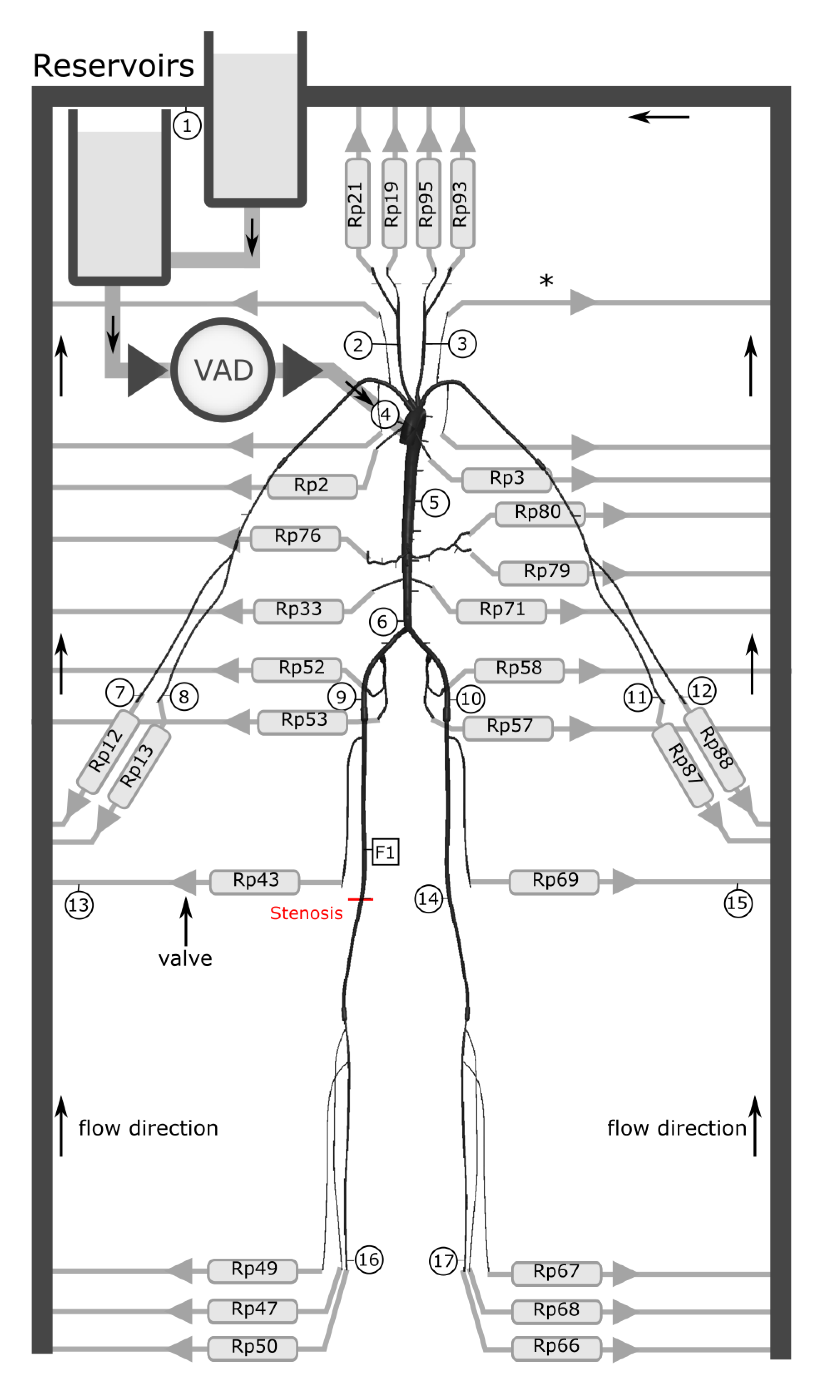
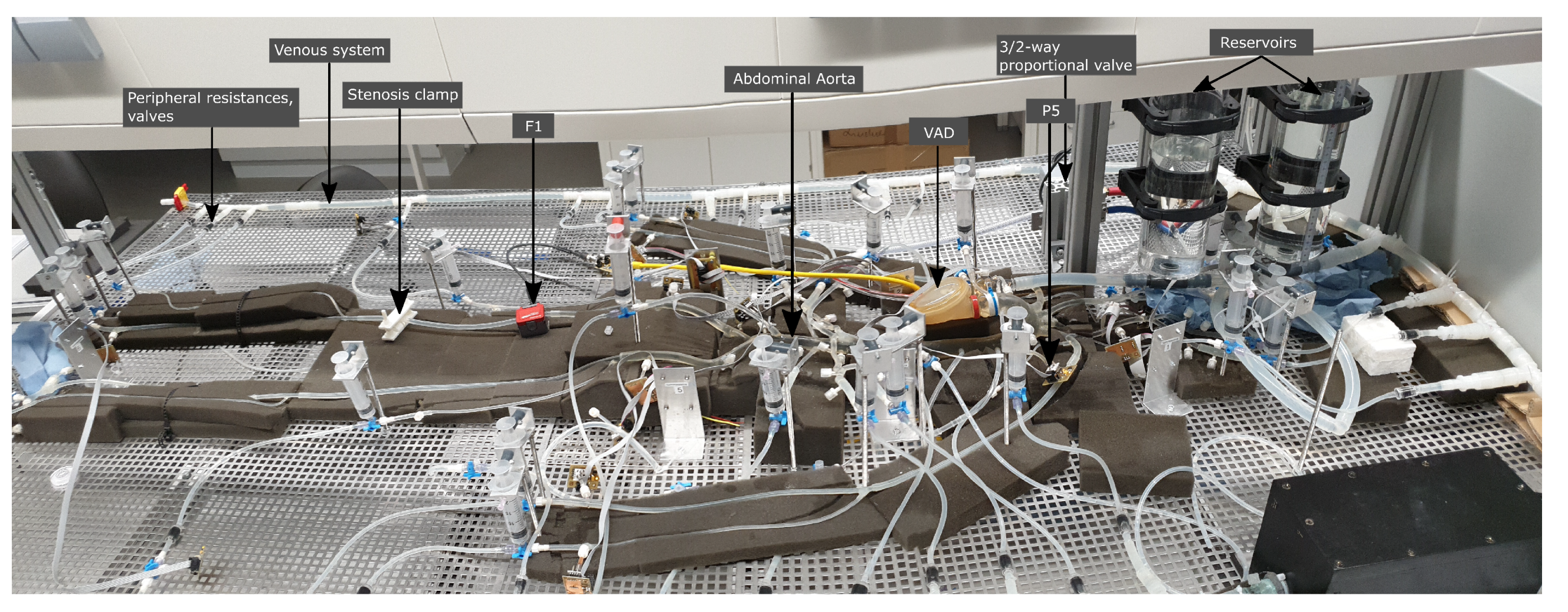
2.1. Cardiovascular Simulator

The development process of the simulator was led by six main design criteria with the aim of establishing a modular and flexible simulation environment that can produce large statistical data sets of specific diseases within highly reproducible flow conditions:
1.
Minimisation of the pulse wave reflection with the condition of obtaining realistic wave reflections from peripheral bifurcations and pathologies.
2
Adjustable flow conditions to a wide range of physiological conditions, such as heart rate, systolic pressure, compliance, and peripheral resistances.
3
Measurement of pressure and flow at several locations within the cardiovascular simulator.
4
Improved laboratory conditions for a highly reproducible pressure and flow measurement on a sample.
5
Parametric scripting of ventricular boundary conditions.
6
Persistent data management in a relational database for post-processing.
The multivariate statistical data sets include relevant meta-information about the experiments and are stored in a MySQL database for further analysis. In the context of this study, the data set is made available via MATLAB files for simple community-wide post-processing. MySQL data can be obtained on request.
The experimental setup of the simulator consists of the following main components (see Figure 1): arterial and venous system with valves and reservoirs, heart pump, compliance and peripheral resistance elements and pressure and flow sensors.

2.1.1. Arterial and Venous System
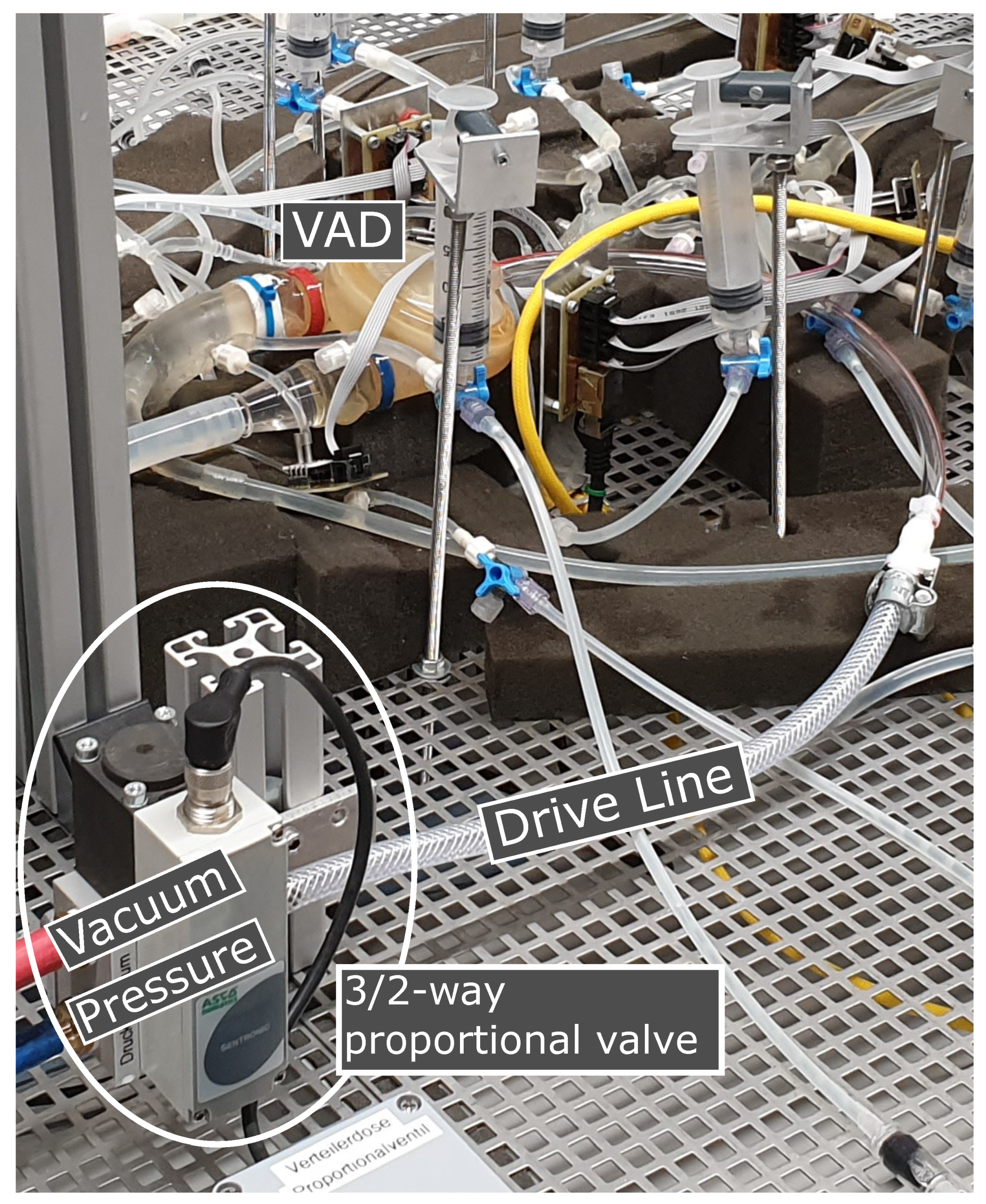
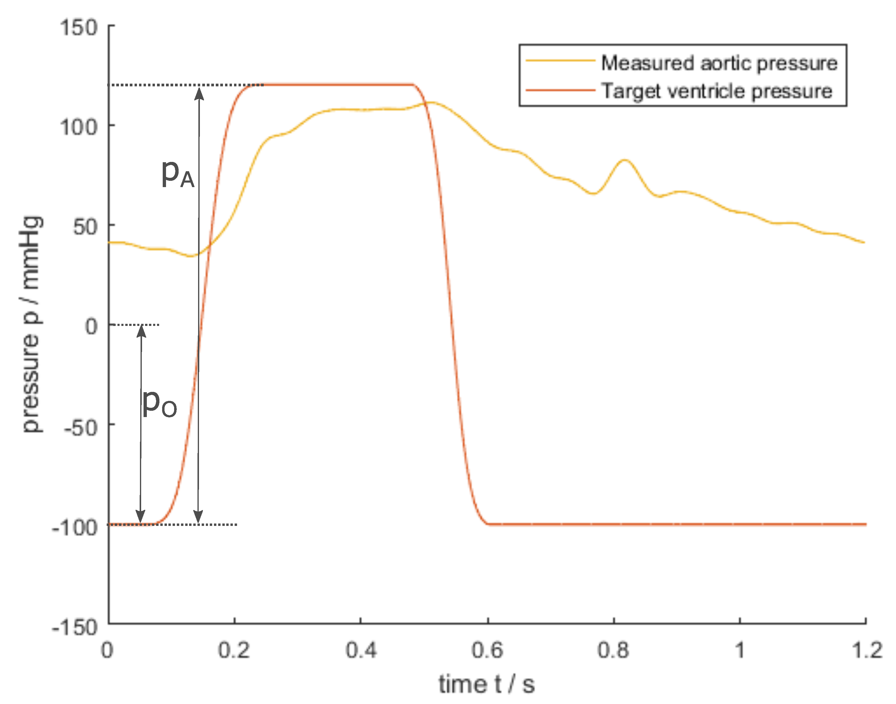
The structure of the cardiovascular simulator contains the major 33 arteries down to an inner diameter of 1.5 mm. This artificial arterial system is realised by a system of silicone tubes that have similar characteristics, such as inner and outer diameter, length and elasticity, as the corresponding human arteries. The structural data for the arterial network were obtained from a real patient-specific MRI scan, which was followed by simplification and smoothing of the boundaries. Thereby, the individual parts of the arterial vascular system (aorta, art. carotis, art. subclavia, art. celiaca, art. iliaca and art. femoralis) were fabricated and assembled using injection moulding. The other parts of the arterial system were made from standard silicon tubes due to the low vessel complexity and diameter. The whole vascular system is bedded on individually shaped PU–foam blocks to ensure proper anatomical tethering. In addition to the arterial vascular system, the simulator includes a venous return system and two reservoirs connecting the venous and arterial system (see Figure 1 and Figure 2).
Because measurements are only performed on the arterial vascular system, a detailed mapping of the venous system was omitted and, instead, a simple feedback from the individual peripheral arteries to the reservoirs was realised. Both reservoirs are filled with V R = 985 mL of fluid, thus creating a hydrostatic pressure offset p h = 14.42 mmHg throughout the model cardiovascular system. The system’s diastolic blood pressure, p ˇ , is set by a combination of the peripheral flow resistances, R p , and the level in the reservoirs. The viscosity and density of the fluid in the simulator are adjusted to achieve physiological values for human blood using a water–glycerine mixture (approx. 60/40 weight %), which has a resulting density of ρ = ( 1.094 ± 0.002 ) g/mL and a dynamic viscosity of η = ( 3.88 ± 0.1 ) mPa·s at room temperature ϑ = 22.4 °C. The node numbering of the arterial network refers to the SISCA computational simulation modelling environment [4]. In this software framework for multi-compartment lumped modelling, each peripheral node number (see Figure A3) represents a flow resistance Rp in Figure 1. The corresponding Table A2 contains measurements and estimations for the vessel diameter d, length l, wall thickness h and elastic modulus E.

2.1.2. Heart Pump

The simulator in-flow conditions at the heart node were realised by a pneumatically driven medical ventricular assist device (VAD) diaphragm pump (Medos Stolberg, Germany) with a maximum stroke volume of 80 ml, which provides a pulsatile fluid flow through the vascular system in a manner analogous to the left ventricle of the heart. The diaphragm pump is a medical device generally used as an external mechanical circulatory support system, for example, as a bridge for heart transplant patients, and it is suitable to create a pulsatile and heart-like pumping behaviour [21]. The diaphragm pump contains two heart valves and is controlled by a 3/2-way proportional valve (Series 614, Sentronic) that outputs the pressure for the drive line (see Figure 3). The proportional valve applies the resulting pressure of a defined pressure curve by mixing an applied relative underpressure of p u = 0.4–0.7 bar and an overpressure of p o = 1 bar. The vacuum pressure is generated by a pressure-controlled vacuum pump and stored in a 40 L reservoir to reduce long-term drift during systole and realise long simulation times with stable pressure conditions. During diastole, the air side of the diaphragm pump is subjected to vacuum pressure reducing the air chamber volume; thus, the membrane moves toward the air side, and the ventricle is filled. The fluid is transported into the system by applying overpressure to push the medium out of the VAD through the arterial outlet.

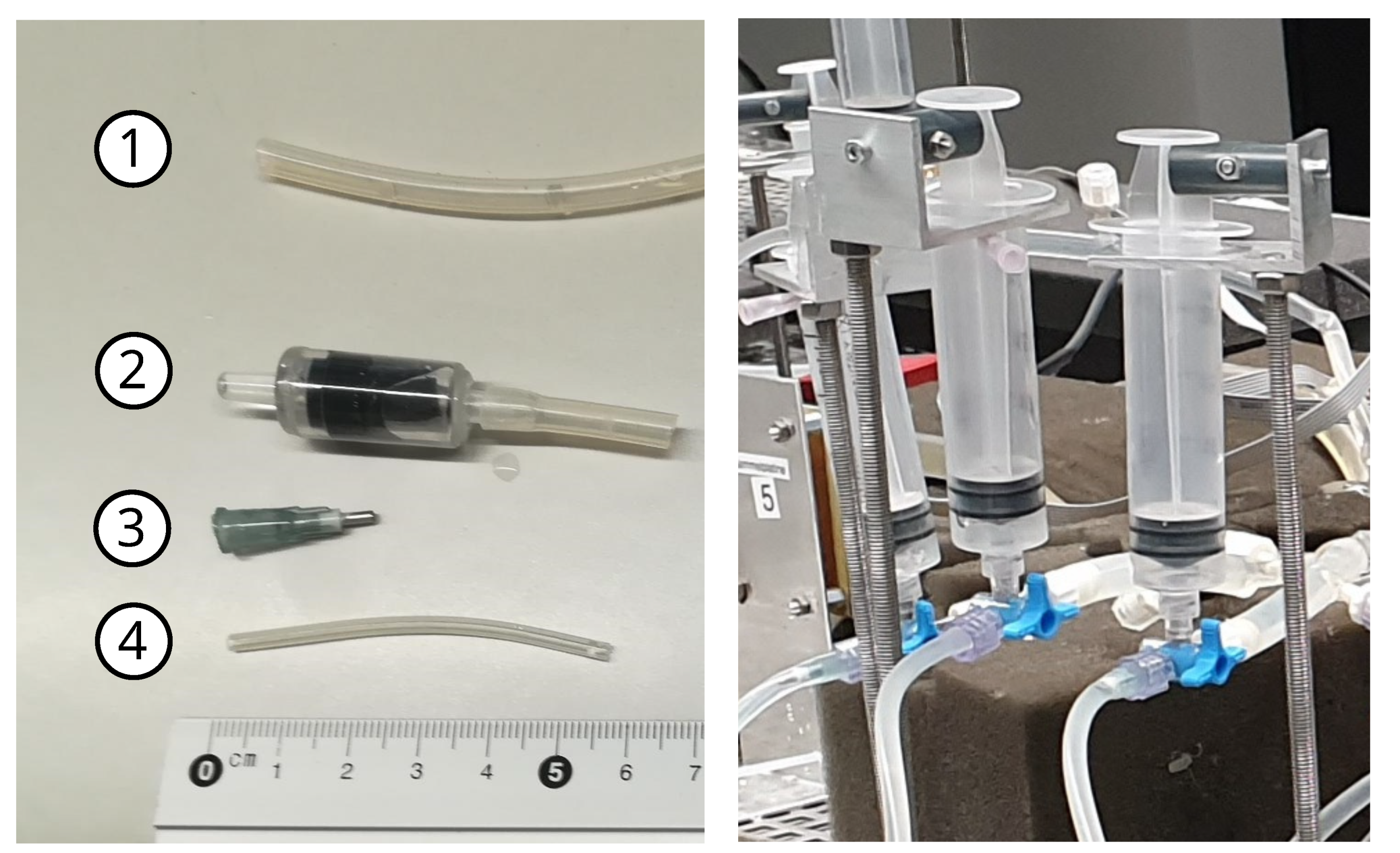
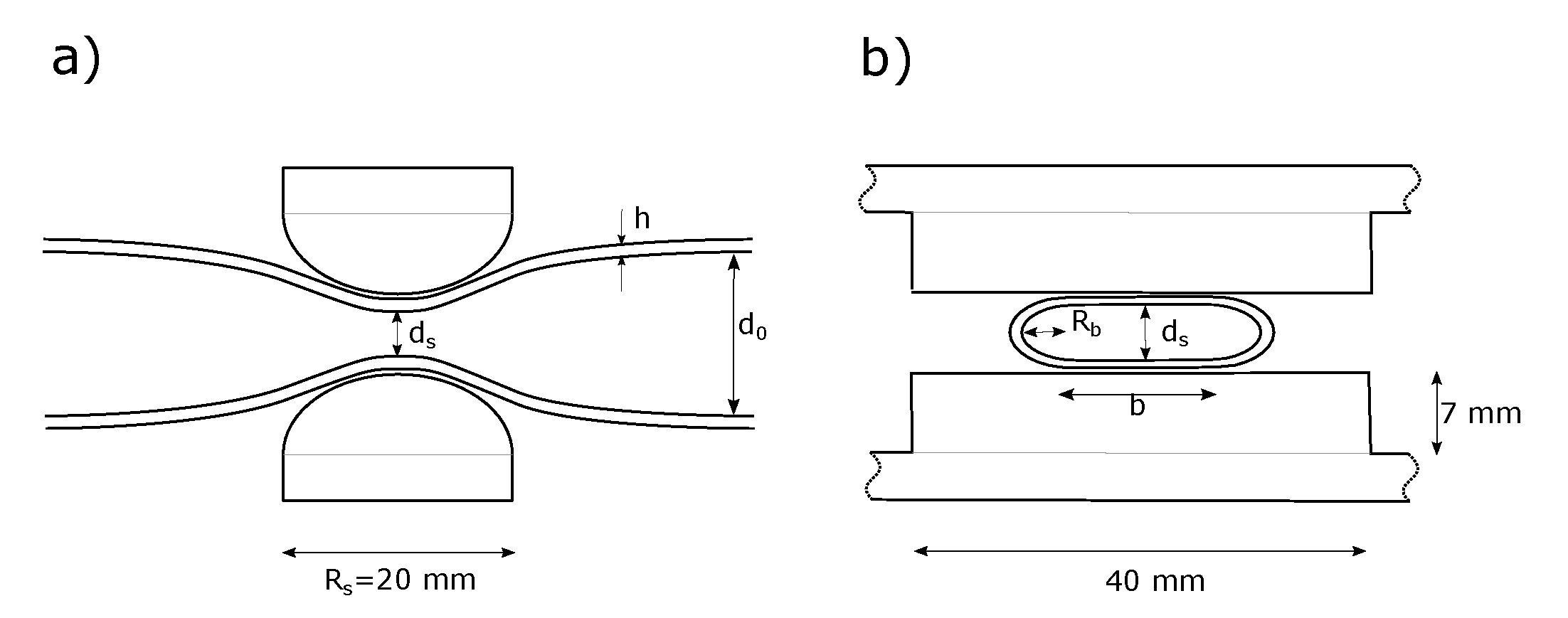
2.1.3. Peripheral Resistance and Compliance

The physiological flow resistance of human arterioles and capillaries is modelled by additional small tubes inserted into the peripheral arteries, which open into the venous system (see Figure 4). The peripheral resistance consists of the outer tube, a cannula with a small inner tube and a check valve. The length of the inner tubes was adjusted according to the physiological flow resistance of the arterial branch. Capillary flow resistance values were reproducibly generated downstream of each vessel end; the relative group values are found in Table 1. Check valves were integrated to prevent the backflow of fluid from the venous to the arterial system. These check valves are analogous to the venous valves in the human body, which prevent back flow in case of venous overpressure at the transition of the flow wave into the venous system. The peripheral viscous flow resistance is defined as
R p = Δ p q ,
where Δ p is the pressure difference, and q represents the volume flow.
The peripheral resistances of the boundary nodes were measured by defining regional groups such as the legs, arms, organs, and head. Table 1 shows the results in relation to the total peripheral resistance of the arterial system R p = ( 1.94 ± 0.02 ) · 10 8 Pa·s/m3 at the given viscosity (for detailed measurement description, see Appendix Peripheral Resistance Measurement).
Compliance was adjusted and compensated for by syringes integrated vertically at the transition to the venous tube system (see Figure 4). These syringes were filled with a defined volume of air and thus created an artificial, additional distensibility of the respective vessels (all syringes were set to an air volume of V p x = 2 mL, except at the peripheral nodes: V p 3 = 3 mL, V p 50 = 5 mL and V p 66 = 6 mL; see Figure 1). The syringes can be considered peripheral windkessel elements and affect the total system compliance. Compliance is defined as the extensibility of an artery and can be calculated by
C = Δ V Δ p ,
where Δ p is the change in pressure for a prescribed change in volume Δ V . The total systems compliance C = ( 0.32 ± 0.01 ) mL/mmHg was measured by adding a defined volume to the arterial system using a syringe connected via a luer-lock connector (for details, see Figure A2).

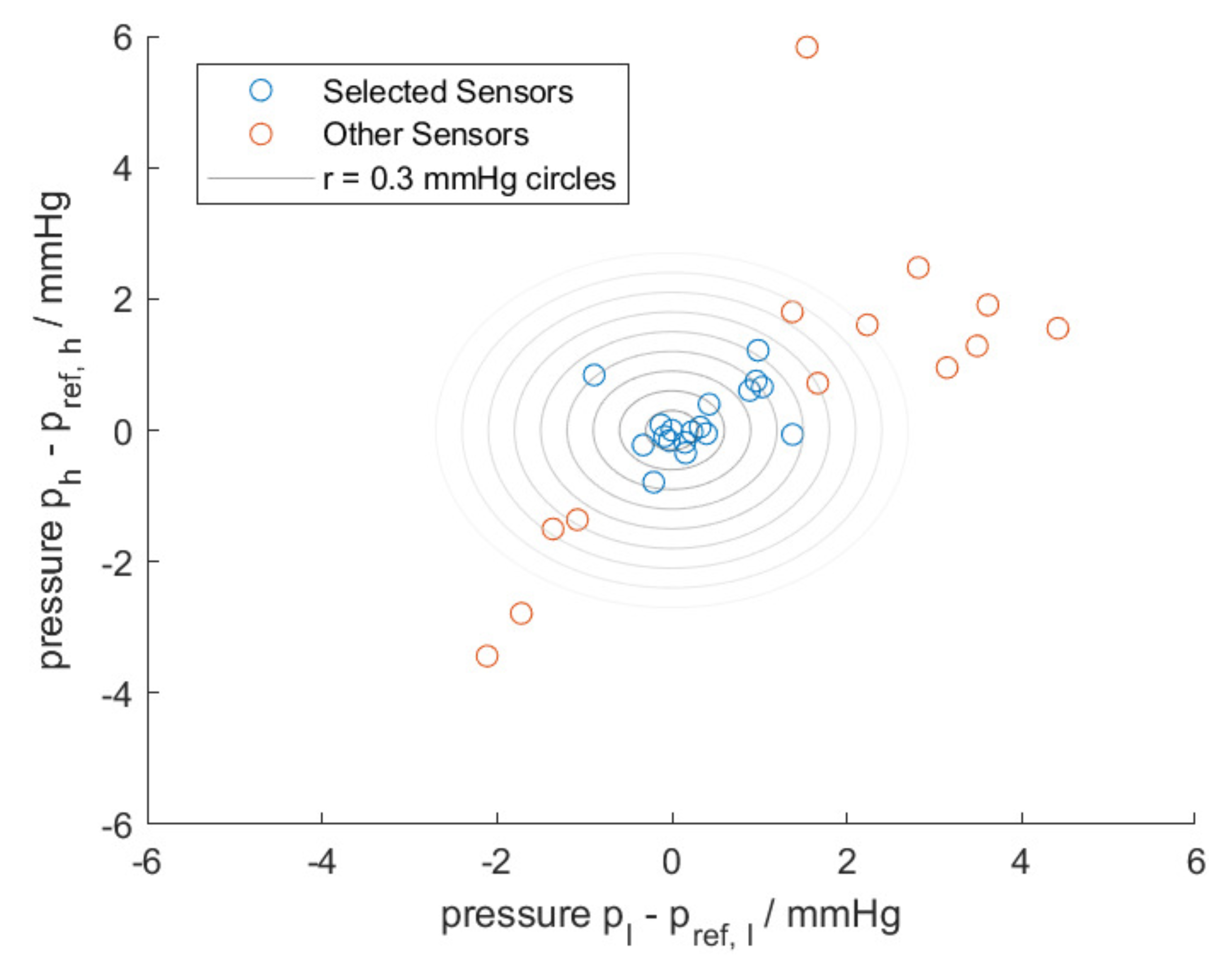
2.1.4. Pressure and Flow Sensors

The pressure and flow were measured as a function of time; that is, p ( t ) and q ( t ) were measured at different locations in the system. Therefore, 17 pressure sensors (AMS 5812, 0050-D-I, inverted, fluid resistant) and a clamp-on medical grade ultrasonic-based flow sensor (SONOFLOW CO.55/060) were used to measure the flow velocity and the pressure in the system at predefined locations (see Figure 1 and Figure 2, label F1 and 1–17). Specific locations of the pressure and flow sensors are shown in the schematic in Figure 1. All sensors were calibrated prior to measurement. Detailed measurement setup and calibration results are given in Figure A1.

2.2. Measurement Setup and Procedure

For each measurement scenario, the pressure and flow were measured at 17 + 1 predefined locations, respectively (see Figure 1). The input heart curve was chosen to be a trapezoidal curve (see Figure 5), which was parametrised by an amplitude, offset, heart frequency and start and end of the ascending/descending slope (see Equation (3)). All measurements were acquired with a heart rate of H R = 50 bpm and a maximum pressure amplitude of p A = 220 mmHg with a negative offset of p O = 100 mmHg. The trapezoidal curve was generated on a normalised time scale t ˜ = t / T , where T is the temporal period for the heart rate.
p i n ( t ˜ ) = p O 0 t ˜ t ˜ a , 1 p O + t ˜ t ˜ a , 1 t ˜ a , 2 t ˜ a , 1 p A t ˜ a , 1 t ˜ t ˜ a , 2 p O + p A t ˜ a , 2 t ˜ t ˜ d , 1 p O + p A t ˜ t ˜ d , 1 t ˜ d , 2 t ˜ d , 1 p A t ˜ d , 1 t ˜ t ˜ d , 2 p O t ˜ d , 2 t ˜ 1
A linear raise was created between t ˜ a , 1 = 0.1 and t ˜ a , 2 = 0.15 followed by a plateau and a descent between t ˜ d , 1 = 0.45 and t ˜ d , 2 = 0.5 . The resulting curve was smoothed by MATLAB’s smoothdata function with a window length of 0.1 and rescaled along the time axis according to the applied heart rate (see Figure 5). The measurements were performed over a period of 60 s to guarantee steady-state conditions and were acquired using a 16-bit data acquisition PCI card (National Instruments, Austin, TX, USA) at sampling frequency of 1000 Hz per channel. The data acquisition software was entirely written in MATLAB. The measurement data and meta-information were stored in a MySQL database for further analysis.

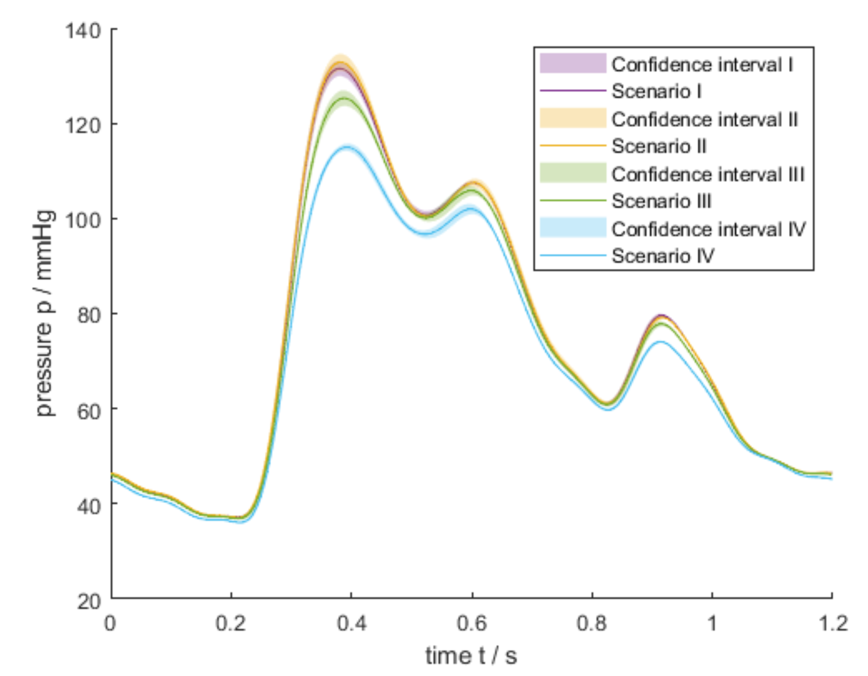
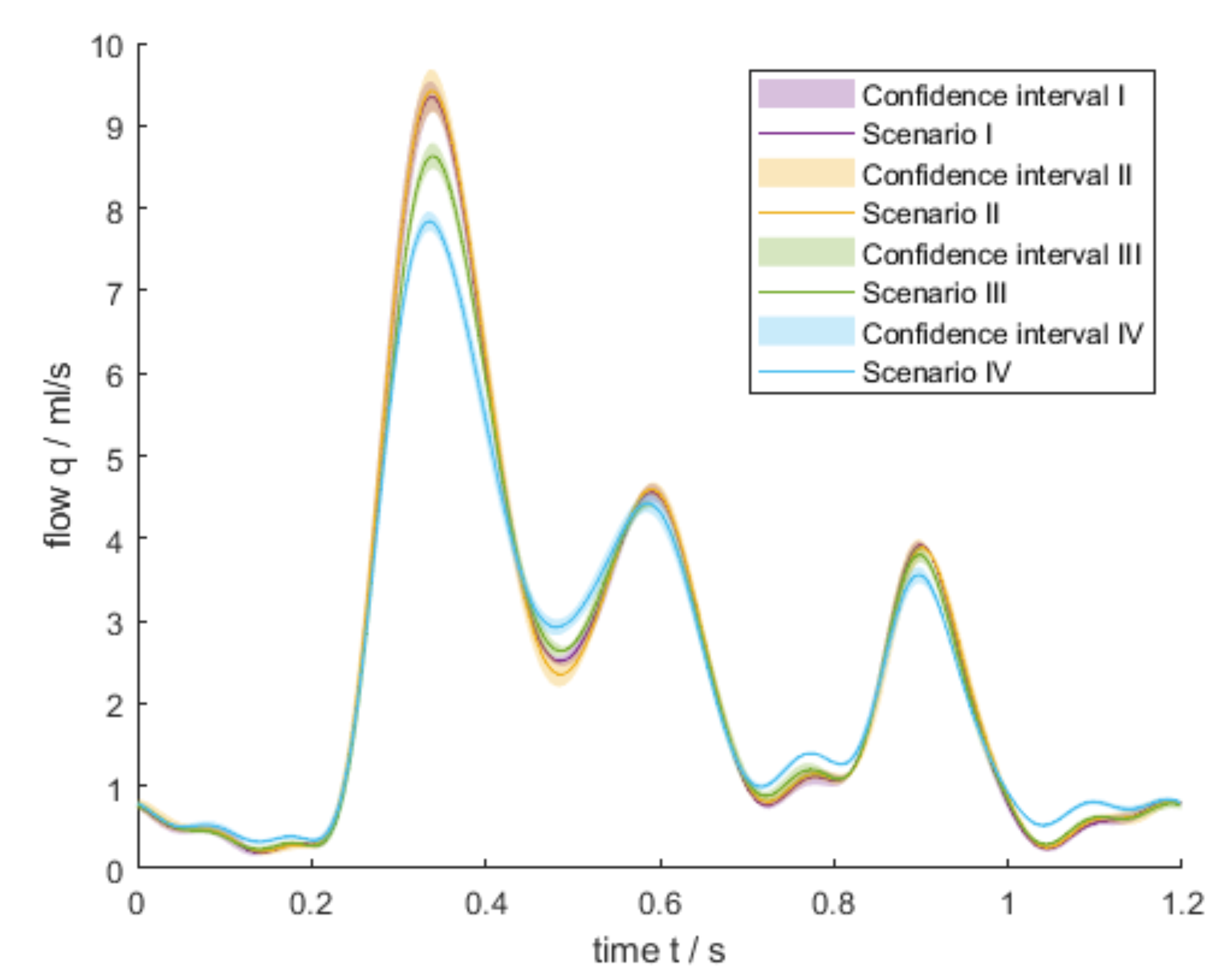
2.3. Measurement Scenarios

The influence of stenoses on the pressure and flow in the cardiovascular system was investigated by simulating different measurement scenarios under healthy and pathological conditions. The healthy state serves as the reference without artificial stenoses. In the pathological setup, an artificial stenosis in art. femoralis 20 cm downstream of the knee (see Figure 1) was chosen. The artery was squeezed, reducing one axial dimension to a fraction between 3.3% and 25% to obtain different degrees of stenosis (see Table 2). This setting does not directly correspond to the clinical situation, where the stenosis cross-section is circular. In this study, the percent reduction of the artery is defined through the area change and the change in diameter. The shape of the stenosed artery in squeezed form (see Figure 6) is described by a rectangle with two attached half circles [22], and the cross-sectional area can be written as A 2 = b d s + ( d s / 2 ) 2 π , where b is the width of the rectangle, and d s the squeezed inner diameter, as seen in Figure 6. For negligible bending resistance in a thin-walled tube, the circumference remains unchanged when squeezing the tube; in this case, one can express the ratio A 2 / A 1 as a function of the ratio δ = d s / d 0 , where A 1 = ( d 0 / 2 ) 2 π is the cross-sectional area of the unsqueezed artery, and d 0 is the initial inner diameter:
A 2 A 1 = 2 δ δ 2 ,
for δ [ 0 ,   1 ] .
All stenoses were established using a 3D-printed clamp (see Figure 2 for the printed object and Figure 6 for the cross-section).

3. Results

The resulting data set is structured into four *.mat files, one per scenario. Each file contains 18 pressure signals and one flow signal; in total, the data set contains 76 signals. The data set and a detailed description are available at [20]. The following subsections describe the properties and results.

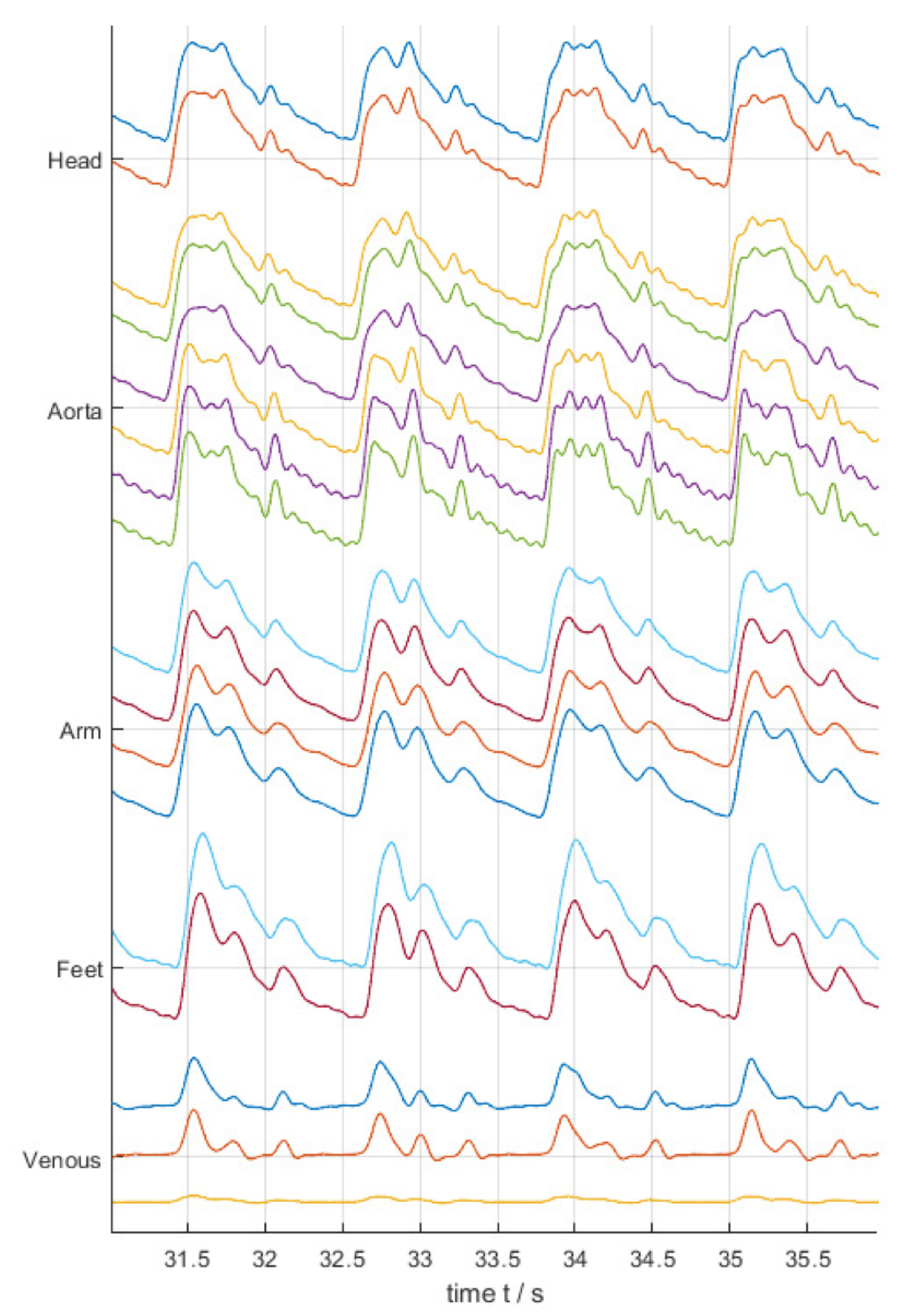
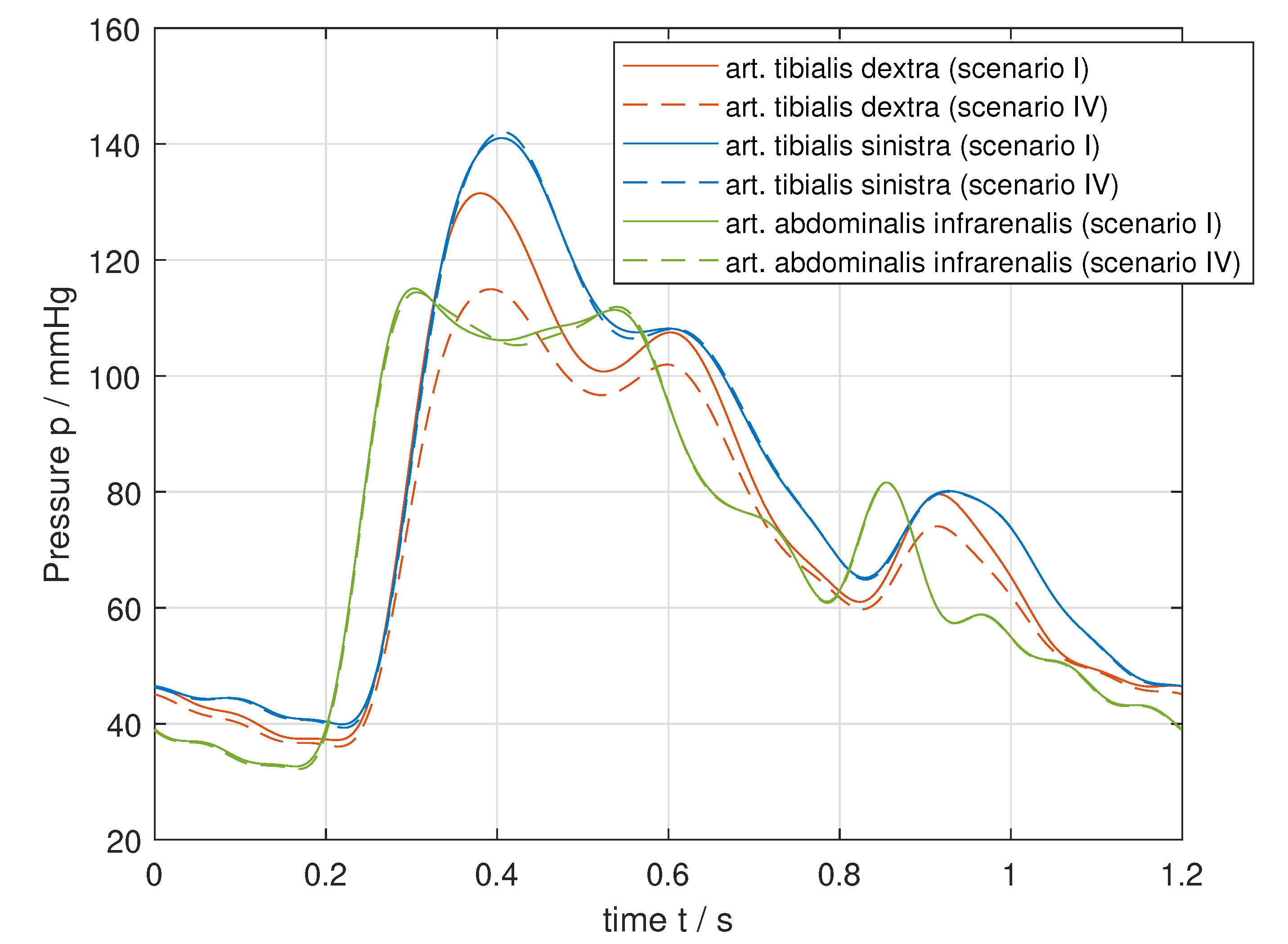
3.1. Pressure Waves along the Arterial Network

Figure 7 shows the entire set of pressure curves along the arterial system under healthy conditions. Due to wave reflections of discontinuities, the pressure waves clearly change their shape while propagating through the arterial system. As expected, a short time delay between aortic and peripheral waves is observed (transit time) that manifests according to the wave velocity in the arterial network. The pressure amplitude increases in the peripheral vessels, which is in agreement with the pulse wave amplification observed in the in vivo measurements.

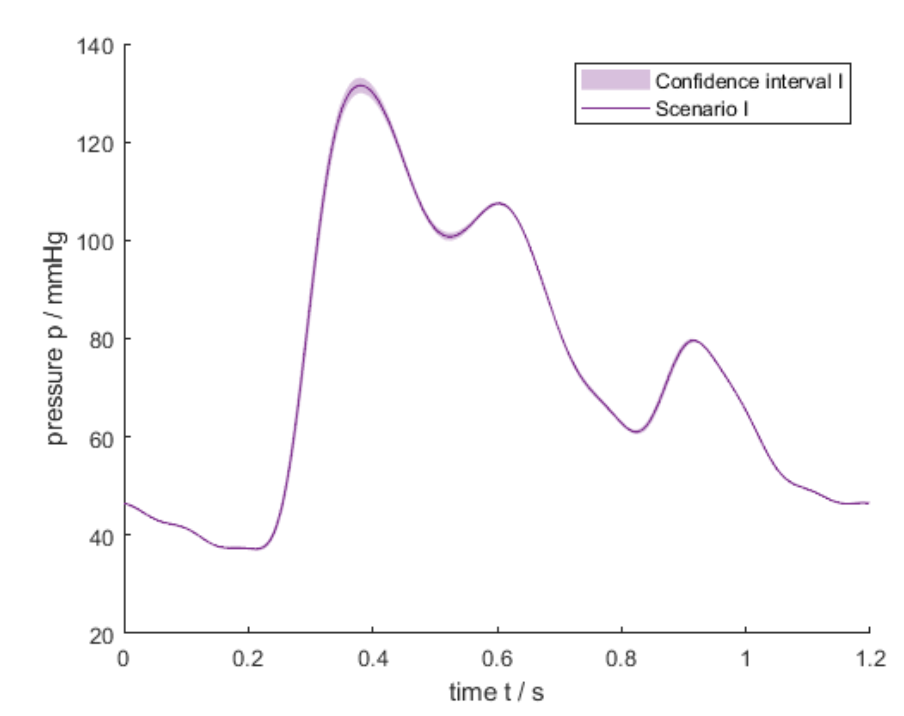
3.2. Scenario I—Healthy Conditions

Figure 8 shows the pressure wave at art. tibialis dextra under normal physiological conditions. The result is similar to in silico simulations and literature in terms of waveshape and specific wave features such as the dicrotic notch and peripheral steeping.
After the systolic rise to the peak pressure of p ^ I = 132 mmHg, the blood pressure drops until the aortic valve closes, resulting in a dicrotic notch in the decaying pressure wave. This notch (incisure) is also found in human pressure waves. Subsequently, the pressure falls to a diastolic level of about p ˇ I = 37.2 mmHg, which is much lower than it would be physiologically.
Figure 8, Figure 9 and Figure 10 contain confidence intervals calculated by the standard deviation of coherent averages; that is, five averaging windows of the size of eight periods were used. The intervals represent the point-wise standard deviation and show the temporal variation within the pressure waves. The confidence interval along the pressure waves is small but increases at the systolic peak values and the discrotic notch. The mean value of the standard deviation of the systolic/diastolic peak values for pressure and flow for each scenario are given in Table 3.

3.3. Scenarios II–VI—Pathological Conditions

The pathological conditions II–VI are based on different degrees of a stenosis in the art. femoralis dextra (see Table 2), corresponding to the measurement results given in Figure 9 and Figure 10.
The pathological scenario II contains a stenosis in art. femoralis with a stenosis degree of δ I I = 25 % . Due to the low degree of the stenosis, there is no obvious difference in the characteristics of the pressure wave. As expected, the stenosis has little effect on the blood pressure: the pressure increases to a systolic peak value of p ^ I I = 133 mmHg, and the diastolic value peaks at p ˇ I I = 37.4 mmHg. The pathological scenario III contains a stenosis with a higher degree of δ I I I = 12.5 % , which causes a decrease of the pressure peak values of the pulse wave at the art. tibialis dextra (see Figure 9). The systolic pressure peak decreases by 6 mmHg to an amplitude of p ^ I I I = 126 mmHg, while the diastolic pressure remains constant at p ˇ I I I = 37 mmHg. Compared to the healthy setup, the shape of the pulse waves distal to the stenosis smoothes due to the reduction of the vessel’s effective diameter by the constriction. As expected, scenario IV has the lowest systolic pressure of all scenarios. Compared to the reference scenario I, the systolic pressure substantially decreases by 16 mmHg to a peak value of p ^ I V = 115.8 mmHg. The mean pressure values for each scenario are given in Table 3. With increasing stenosis degree, the mean pressure p ¯ decreases, but the decrease is not as large as the decrease in the peak values p ^ . The difference in the mean pressure between scenarios I and IV is only 4.3 mmHg, which can be explained by the fact that although the systolic pressure decreases, the diastolic pressure remains at the same level for all scenarios.
Figure 10 shows the flow waves at the art. profunda femoris dextra for all measurement scenarios. The peak values of the flow velocity for the healthy state (scenario I) are q ^ I = 9.4 mL/s, and they reduced as expected for all pathological conditions q ^ I I = 9.3 mL/s, q ^ I I I = 8.6 mL/s and q ^ I V = 7.8 mL/s. Consequently, the flow velocity within the diseased vessel decreases with an increasing degree of the stenosis. The mean flow values for each scenario are given in Table 3. In contrast to the peak values, the mean flow remains almost constant.
Finally, Figure 11 shows the influence of the stenosis on different adjacent arteries such as art. abdominalis infrarenalis and art. tibialis dextra and sinistra. Scenario I has no stenosis δ I = 100 % ; scenario IV has a stenosis of degree δ I V = 3.3 % . The pressure wave measured in the right foot decreases, while the pressures measured in the aorta and in the left foot remain virtually unchanged.

4. Discussion

The purpose of this study was the development and validation of a patient-specific in vitro hardware simulator to generate parametric data sets under healthy and pathological conditions for computational model validation. Different hardware simulators have been developed to investigate various theses; the three-dimensional arterial structures differ in complexity, the type of heart pump, the number of sensors and properties such as compliance and peripheral resistances. In [16], the simulator drive consists of two pneumatically driven VADs representing the right and the left ventricle. In [26], a Harvard pulsatile pump is used. Furthermore, both hardware simulators [16,26] contain detailed arterial networks covering 37 major arteries of the human body. In contrast, hardware simulators designed to test and validate VADs include an arterial network of low complexity and a simple, functional drive. The simulator in this work is pneumatically driven by one VAD to provide a pulsatile fluid flow through the vascular system. The arterial network contains a detailed arterial network with adjustable elements regarding heart rate, systolic/diastolic pressure, compliance and peripheral resistances. The simulator provides one flow sensor and 17 pressure sensors at different locations that enable a detailed evaluation of the wave propagation. Due to material properties, the total arterial compliance of the simulator is C = ( 0.32 ± 0.01 ) mL/mmHg and lower than in vivo. The total peripheral resistance is R p = ( 1.94 ± 0.02 ) · 10 8 Pa·s/m3. The low compliance evokes that the stiffness of arteries is higher than in vivo, which indicates an atherosclerotic, high-blood-pressure patient. In contrast, the arterial compliance in [16] was adjusted to 1.0 mL/mmHg, and no peripheral compliances are included in [26]. As shown in the results section, the properties of the pressure waves within the simulator are similar to those of in vivo measurements. The waveshape and specific wave features such as the discrotic notch, peripheral steeping and translational pressure drop are observed. Due to wave reflection at discontinuities and compliance variation of the vessels, the shape of the pressure changes while propagating through the system.
The influence of a stenosis and its degree on the pulse wave in the circulatory system was investigated. As expected, the results show that the pressure after the diseased vessel decreases with an increase in the degree of stenosis. The flow measurements show similar results (see Figure 10): the flow decreases for a higher degree of stenosis, as expected. These results conform with results provided by other hardware simulators [14,27]. The influence of stenosis on different arteries was also examined. Figure 11 shows that the stenosis at art. femoralis dextra only impacts the diseased vessel in the right leg, where the pressure decreases. The pressure wave in the aorta and the left leg remain virtually unchanged. The measurements under physiologic and pathological conditions confirm the validity of the in vitro hardware simulator. Certain limitations of the results of this study could be addressed in future research. The first limitation concerns the low compliance of the arterial system and the peripheral resistances, which are too high. The compliance could be adjusted by a higher volume of syringes within the system. The impact of the different resistance elements, such as inner tubes and valves, could be adjusted to create more physiological peripheral resistance. A further potential limitation is the measured pressure waves, which are affected by a broad frequency range of noise. The noise is created by the vibrations of the system components due to the pumping process of the VAD. This could be fixed in future research by embedding the tube system within PU–foam blocks. Moreover, the diastolic pressure of about 40 mmHg is too low compared to in vivo measurements. The reason for this may be the low compliance and the high peripheral resistance within the system. In conclusion, the present study has provided measurement data that support the validation of computational models. The improvement of the understanding of the pathology and the validation of computational models will enable interpretation in a clinical setting. Future research could extend the current findings by generating a data set with the hardware simulator that can be used to develop and test algorithms for stenosis detection and localisation.

5. Conclusions

In this study, an in vitro cardiovascular hardware simulator was developed and validated to better understand blood pressure and flow under healthy and pathological conditions. Physiological flow conditions are adjustable across a wide range by changing heart rate, systolic/diastolic pressure, compliance and peripheral resistance parameters. The pressure and flow waves show similar waveforms as the in vivo measurements, and the pressure and flow waves show the expected behaviour in the case of different locations and degrees of stenosis. This work provides measurement data about healthy and pathological conditions such as stenoses to the research community to support the validation of computational models.

Author Contributions

Conceptualization, M.W., A.M. and S.B.; methodology, M.W., A.M. and S.B.; software/hardware, P.S., M.W., B.L. and M.O.; validation, M.W., A.M. and S.B.; formal analysis, A.M. and S.B.; investigation, M.W. and A.M.; resources, S.B.; data curation, M.W., A.M. and S.B.; writing—original draft preparation, M.W., A.M. and S.B.; writing—review and editing, S.B.; visualization, M.W.; supervision, S.B.; project administration, S.B.; funding acquisition, S.B. All authors have read and agreed to the published version of the manuscript.

Funding

This research received no external funding.

Institutional Review Board Statement

Not applicable.

Informed Consent Statement

Not applicable.

Data Availability Statement

Data is available online on zenodo platform at https://doi.org/10.5281/ZENODO.6415276 (accessed on 10 September 2022).

Conflicts of Interest

The authors declare no conflict of interest.

Appendix A

Appendix A.1. Calibration Measurements

All pressure and flow sensors used in this study were calibrated to ensure valid measurement data.

Appendix A.2. Calibration of Pressure Sensors

The pressure sensors were calibrated through a two-point calibration measurement. A bag filled with water was set to a defined hydrostatic pressure. This pressure corresponds to a water column of p h = 820 m m H 2 O = 61.8 mmHg. Subsequently, the hydrostatic pressure was set to p l = 0 mmHg compared to the atmospheric pressure for the second point for the calibration measurement. A reference sensor, p r e f , was present in each calibration measurement to compare the measurement values. The results of the calibration measurement for each sensor are shown in Figure A1. All sensors lie within a maximum deviation of ± 1.5 mmHg.

Appendix A.3. Calibration Flow Sensor

The flow sensor was calibrated through a two-point calibration measurement, where the volume difference between the steady state and running system was evaluated at location F1 (see Figure 1). Volume integration was completed by disconnecting the reservoirs and determining the fluid amount per time. Subsequently, a correction factor of 4.8 and the mean flow velocity were calculated.

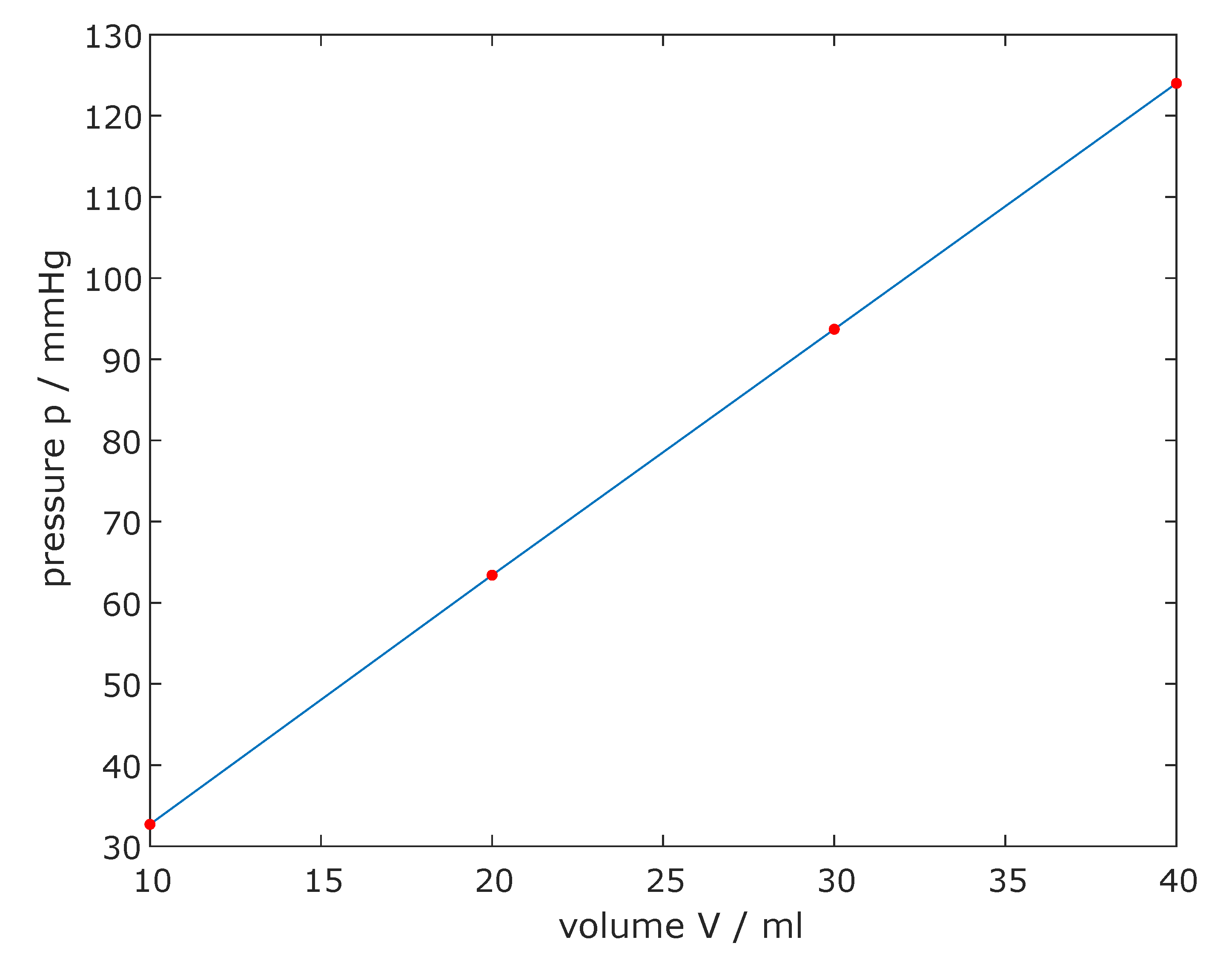
Appendix A.4. Compliance

The system compliance was evaluated by measuring the pressure changes resulting from consecutive fluid injections of Δ V = 10 mL into the closed arterial system (see Table A1).
Figure A1. Scatter plot of calibrated pressure sensors compared to the reference sensor p r e f .
Data 07 00145 g0a1
Table A1. Pressure-volume measurements and compliance evaluation of the arterial system obtained by consecutively fluid injections of Δ V = 10 mL.
No. Δ p ¯ (mmHg) Δ V (mL)C (mL/mmHg)
132.7100.3058
230.7100.3257
330.3100.3300
430.3100.3300
The resulting pressure–volume relationship is plotted in Figure A2; the linear slope implies a proportional relationship in the measurement region as expected. Consequently, the total arterial compliance can be calculated by Equation (A1) using the mean pressure difference p ¯ .
C = Δ V Δ p ¯ = 10 mL 31 mmHg = 0.32 mL / mmHg

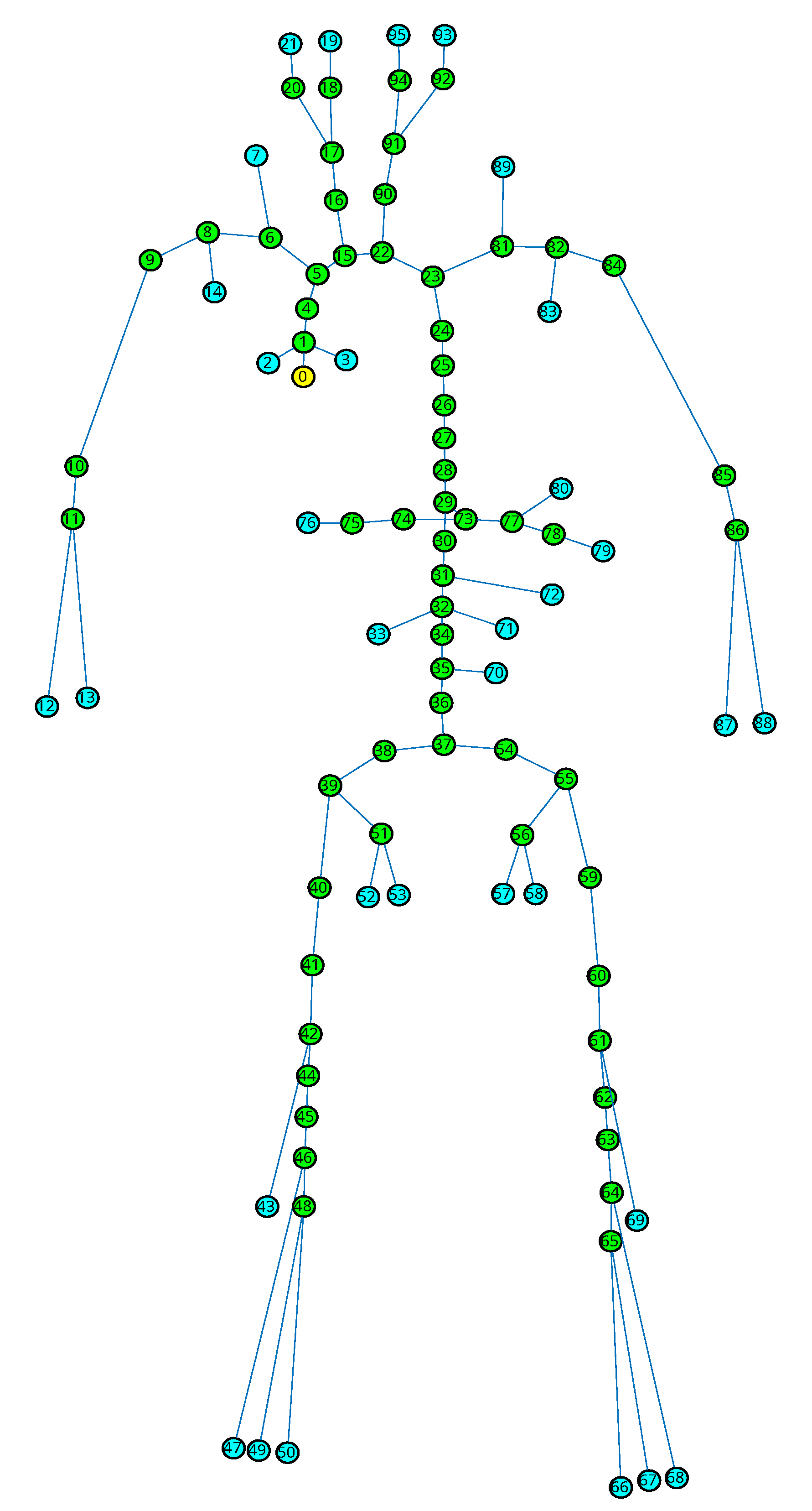
Appendix A.5. SISCA Model

The node structure of the hardware simulator refers to a computational simulation model realised in the SISCA modelling environment [4]. The node numbering of the arterial tree in SISCA is realised by a depth-first search tree. The SISCA software and the simulation model (shown in Figure A3) are available at [28].

Appendix A.6. Overview of the Structural Properties of the MACSim

Table A2 shows an overview of the properties length l, diameter d, wall thickness h and elasticity E of the corresponding SISCA node ID.
Figure A2. Pressure–volume relationship of the arterial network for an injection of a volume of Δ V = 10 mL. Total arterial compliance refers to the slope of the curve.
Data 07 00145 g0a2
Table A2. Structural properties of the MACSim corresponding to SISCA node IDs.
Node IDL (m)h (m)d (m)E (Pa)
10.020.00150.0256,700,000
20.0670.00050.0041,650,000
30.080.00050.0041,650,000
40.010.00150.0256,700,000
50.0520.00150.0256,700,000
60.0490.0010.016,700,000
70.140.00050.00151,650,000
80.0160.0010.016,700,000
90.0530.0010.016,700,000
100.350.0010.0061,650,000
110.0210.0010.0041,650,000
120.3250.0010.0041,650,000
130.3450.00050.0031,650,000
140.0950.00040.00151,650,000
150.0130.00150.0256,700,000
160.110.00050.00656,700,000
170.0450.00050.00656,700,000
180.0540.00050.0046,700,000
190.0360.00050.0046,700,000
200.060.00050.0066,700,000
210.0290.00050.0066,700,000
220.0120.00150.0286,700,000
230.010.00150.0286,700,000
240.0020.00150.0286,700,000
250.050.00150.0256,700,000
260.050.00150.0216,700,000
270.050.00150.026,700,000
280.0490.00150.0196,700,000
290.0270.00150.0196,700,000
300.020.00150.0186,700,000
310.0060.00150.0176,700,000
320.0280.00150.0166,700,000
330.080.00050.0041,650,000
340.0210.00150.0166,700,000
350.0310.00150.0156,700,000
360.0180.00150.0156,700,000
370.0150.00150.0146,700,000
380.0410.00010.016,700,000
390.020.00010.016,700,000
400.0940.00010.016,700,000
410.0150.00010.016,700,000
420.0390.00010.0081,650,000
430.280.00050.0031,650,000
440.130.00050.0081,650,000
450.340.00050.0061,650,000
460.0350.0010.0041,650,000
470.4250.00050.0021,650,000
480.0490.0010.0041,650,000
490.3750.00050.0021,650,000
500.360.0010.0041,650,000
510.0730.00050.0066,700,000
520.0550.00050.0066,700,000
530.0630.00050.0066,700,000
540.0410.00010.016,700,000
550.020.00010.016,700,000
560.0730.00050.0066,700,000
570.0630.00050.0066,700,000
580.0550.00050.0066,700,000
590.0940.00010.016,700,000
600.0150.00010.016,700,000
610.0390.00010.0081,650,000
620.130.00050.0081,650,000
630.340.00050.0064,000,000
640.0350.0010.0041,650,000
650.0490.0010.0041,650,000
660.360.0010.0041,650,000
670.3750.00050.0021,650,000
680.4250.00050.0021,650,000
690.280.00050.0031,650,000
700.01670.00050.0051,650,000
710.0080.00050.0041,650,000
720.01750.00050.0051,650,000
730.0250.0010.0056,700,000
740.0270.0010.0056,700,000
750.0250.0010.0056,700,000
760.0470.0010.0056,700,000
770.0540.0010.0056,700,000
780.010.0010.0056,700,000
790.0340.0010.0056,700,000
800.0380.0010.0056,700,000
810.0490.0010.016,700,000
820.0160.0010.016,700,000
830.0950.00040.00151,650,000
840.0530.0010.016,700,000
850.350.0010.0061,650,000
860.0210.0010.0041,650,000
870.3450.00050.0031,650,000
880.3250.0010.0041,650,000
890.140.00050.00151,650,000
900.110.00050.00656,700,000
910.0450.00050.00656,700,000
920.060.00050.0066,700,000
930.0290.00050.0066,700,000
940.0540.00050.0046,700,000
950.0360.00050.0046,700,000
Figure A3. SISCA network structure of the MACSim.
Data 07 00145 g0a3

Appendix A.7. Peripheral Resistance Measurement

The peripheral resistances were measured by defining different regional groups (see Table 1). The peripheral resistance, R p , of each group was determined by the volume difference between the steady state and the running system. Volume integration was completed by disconnecting the reservoirs and determining the fluid amount per time. Only the corresponding arteries in the defined group were connected to the arterial network of the simulator by closing all three-way valves to other arteries. Given the volume and pressure difference, the peripheral resistance for each group was calculated using Equation (1). The peripheral resistance is built by different elements (see Figure 4), which all possess static values, except for the resistance of the small inner tubes, which varies according to their length. The lengths of the small inner tubes to the corresponding boundary node IDs are shown in Table A3.
Table A3. Values for the length, l p , of the peripheral resistance elements ( d = 1 mm) for each boundary node, ID, referring to the R p defined in Figure 1.
Node ID l p (mm)
219.8
319.4
127
138.3
192.4
212.7
3319.5
4313
478.3
4917.6
5017.2
5219.4
5319.4
5719.4
5819.5
6617.6
6717.2
684.7
6913.3
708.3
7119.4
728.2
768.4
795.4
808.4
878.9
887
932.3
952.1
7/
89/
14/
83/

References

  1. Fowkes, F.G.R.; Rudan, D.; Rudan, I.; Aboyans, V.; Denenberg, J.O.; McDermott, M.M.; Norman, P.E.; Sampson, U.K.A.; Williams, L.J.; Mensah, G.A.; et al. Comparison of global estimates of prevalence and risk factors for peripheral artery disease in 2000 and 2010: A systematic review and analysis. Lancet 2013, 382, 1329–1340. [Google Scholar] [CrossRef]
  2. Mathiesen, E.B.; Joakimsen, O.; Bønaa, K.H. Prevalence of and risk factors associated with carotid artery stenosis: The Tromsø Study. Cerebrovasc. Dis. 2001, 12, 44–51. [Google Scholar] [CrossRef] [PubMed]
  3. Quick, C.M.; Young, W.L.; Noordergraaf, A. Infinite number of solutions to the hemodynamic inverse problem. Am. J. Physiol.-Heart Circ. Physiol. 2001, 280, H1472–H1479. [Google Scholar] [CrossRef]
  4. Huttary, R.; Goubergrits, L.; Schütte, C.; Bernhard, S. Simulation, identification and statistical variation in cardiovascular analysis (SISCA)—A software framework for multi-compartment lumped modeling. Comput. Biol. Med. 2017, 87, 104–123. [Google Scholar] [CrossRef] [PubMed]
  5. Gul, R.; Bernhard, S. Parametric uncertainty and global sensitivity analysis in a model of the carotid bifurcation: Identification and ranking of most sensitive model parameters. Math. Biosci. 2015, 269, 104–116. [Google Scholar] [CrossRef] [PubMed]
  6. Quarteroni, A.; Veneziani, A.; Vergara, C. Geometric multiscale modeling of the cardiovascular system, between theory and practice. Comput. Methods Appl. Mech. Eng. 2016, 302, 193–252. [Google Scholar] [CrossRef] [Green Version]
  7. Quarteroni, A.; Ragni, S.; Veneziani, A. Coupling between lumped and distributed models for blood flow problems. Comput. Vis. Sci. 2001, 4, 111–124. [Google Scholar] [CrossRef]
  8. Zenker, S.; Rubin, J.; Clermont, G. From inverse problems in mathematical physiology to quantitative differential diagnoses. PLoS Comput. Biol. 2007, 3, e204. [Google Scholar] [CrossRef] [Green Version]
  9. Garber, L.; Khodaei, S.; Keshavarz-Motamed, Z. The Critical Role of Lumped Parameter Models in Patient-Specific Cardiovascular Simulations. Arch. Comput. Methods Eng. 2021, 29, 2977–3000. [Google Scholar] [CrossRef]
  10. Ježek, F.; Kulhánek, T.; Kalecký, K.; Kofránek, J. Lumped models of the cardiovascular system of various complexity. Biocybern. Biomed. Eng. 2017, 37, 666–678. [Google Scholar] [CrossRef]
  11. Jones, G.; Parr, J.; Nithiarasu, P.; Pant, S. A physiologically realistic virtual patient database for the study of arterial haemodynamics. Int. J. Numer. Methods Biomed. Eng. 2021, e3497. [Google Scholar] [CrossRef] [PubMed]
  12. Boileau, E.; Nithiarasu, P.; Blanco, P.J.; Müller, L.O.; Fossan, F.E.; Hellevik, L.R.; Donders, W.P.; Huberts, W.; Willemet, M.; Alastruey, J. A benchmark study of numerical schemes for one-dimensional arterial blood flow modelling. Int. J. Numer. Methods Biomed. Eng. 2015, 31, e02732. [Google Scholar] [CrossRef] [PubMed] [Green Version]
  13. Vignon-Clementel, I.E.; Chapelle, D.; Barakat, A.I.; Bel-Brunon, A.; Moireau, P.; Vibert, E. Special Issue of the VPH2020 Conference:Virtual Physiological Human: When Models, Methods and Experiments Meet the Clinic. Ann. Biomed. Eng. 2022, 50, 483–484. [Google Scholar] [CrossRef]
  14. Jin, W.; Alastruey, J. Arterial pulse wave propagation across stenoses and aneurysms: Assessment of one-dimensional simulations against three-dimensional simulations and in vitro measurements. J. R. Soc. Interface 2021, 18, 20200881. [Google Scholar] [CrossRef] [PubMed]
  15. Korzeniowski, P.; White, R.J.; Bello, F. VCSim3: A VR simulator for cardiovascular interventions. Int. J. Comput. Assist. Radiol. Surg. 2018, 13, 135–149. [Google Scholar] [CrossRef] [Green Version]
  16. Gehron, J.; Zirbes, J.; Bongert, M.; Schäfer, S.; Fiebich, M.; Krombach, G.; Böning, A.; Grieshaber, P. Development and Validation of a Life-Sized Mock Circulatory Loop of the Human Circulation for Fluid-Mechanical Studies. ASAIO J. 2019, 65, 788–797. [Google Scholar] [CrossRef] [PubMed]
  17. Ferrari, G.; de Lazzari, C.; Kozarski, M.; Clemente, F.; Górczynska, K.; Mimmo, R.; Monnanni, E.; Tosti, G.; Guaragno, M. A Hybrid Mock Circulatory System: Testing a Prototype Under Physiologic and Pathological Conditions. ASAIO J. 2002, 48, 487. [Google Scholar] [CrossRef] [PubMed]
  18. Pugovkin, A.A.; Selishchev, S.V.; Telyshev, D.V. Simulator for Modeling the Cardiovascular System for Testing Circulatory Assist Devices. Biomed. Eng. 2015, 49, 213–216. [Google Scholar] [CrossRef]
  19. Pugovkin, A.A.; Telyshev, D.V. Automated pediatric cardiovascular simulator for left ventricular assist device evaluation. In Proceedings of the 2017 International Siberian Conference on Control and Communications (SIBCON), Astana, Kazakhstan, 29–30 June 2017; pp. 1–4. [Google Scholar] [CrossRef]
  20. Bernhard, S.; Wisotzki, M.; Schlett, P.; Lindner, B.; Mair, A.; Oberhardt, M. In-vitro Major Arterial Cardiovascular Simulator: Benchmark Data Set for in-silico Model Validation. arXiv 2022, arXiv:2204.10005. [Google Scholar]
  21. Thuaudet, S. The Medos ventricular assist device system. Perfusion 2000, 15, 337–343. [Google Scholar] [CrossRef]
  22. Bernhard, S.; Möhlenkamp, S.; Tilgner, A. Transient integral boundary layer method to calculate the translesional pressure drop and the fractional flow reserve in myocardial bridges. Biomed. Eng. Online 2006, 5, 42. [Google Scholar] [CrossRef] [PubMed] [Green Version]
  23. O’Rourke, M.F.; Yaginuma, T. Wave Reflections and the Arterial Pulse. Arch. Intern. Med. 1984, 144, 366–371. [Google Scholar] [CrossRef] [PubMed]
  24. Nielsen, P.E.; Barras, J.P.; Holstein, P. Systolic Pressure Amplification in the Arteries of Normal Subjects. Scand. J. Clin. Lab. Investig. 1974, 33, 371–377. [Google Scholar] [CrossRef]
  25. Murgo, J.P.; Westerhof, N.G.J.; Sa, A. A. Aortic input impedance in normal man: Relationship to pressure wave forms. Circulation 1980, 62, 105–116. [Google Scholar] [CrossRef] [PubMed] [Green Version]
  26. Matthys, K.S.; Alastruey, J.; Peiró, J.; Khir, A.W.; Segers, P.; Verdonck, P.R.; Parker, K.H.; Sherwin, S.J. Pulse wave propagation in a model human arterial network: Assessment of 1-D numerical simulations against in vitro measurements. J. Biomech. 2007, 40, 3476–3486. [Google Scholar] [CrossRef] [PubMed]
  27. Hacham, W.S.; Khir, A.W. The speed, reflection and intensity of waves propagating in flexible tubes with aneurysm and stenosis: Experimental investigation. Proc. Inst. Mech. Eng. Part H J. Eng. Med. 2019, 233, 979–988. [Google Scholar] [CrossRef] [PubMed]
  28. Huttary, R.; Maier, A.; Bernhard, S. agbernhard.lse.thm.de/SISCA, GitLab. 2021. Available online: https://gitlab.com/agbernhard.lse.thm/sisca/ (accessed on 6 April 2022).
Figure 1. Schematic of the experimental setup, including a VAD pump and the vascular model. The resistance elements (grey boxes) with adjacent check valves separate the arterial and venous sections. A water–glycerine mixture (approx. 60/40 weight %) of viscosity η = ( 3.88 ± 0.1 ) mPa·s was used to model the properties of blood at 37 °C. F1 and 1 to 17 represent the measurement locations of the flow and pressure sensors, respectively. The compliance elements (syringes; see Figure 4) are located at the peripheral ends (prior to the peripheral resistances Rp) and at the * marked position, except for Rp52, Rp53, Rp58 and Rp57.
Data 07 00145 g001
Figure 2. Main components of the major arterial cardiovascular simulator (MACSim): 3/2-way proportional valve, VAD, arterial system, venous system and reservoirs, peripheral resistances, and valves.
Data 07 00145 g002
Figure 3. The 3/2-way proportional valve and the VAD. The 3/2-way proportional valve mixes a relative underpressure of p u = 0.4–0.7 bar and an overpressure of p o = 1 bar and applies the resulting pressure to the drive line to control the VAD.
Data 07 00145 g003
Figure 4. Peripheral resistance elements (left), including (1) outer tube, (2) valve, (3) cannula and (4) small tube and compliance element (right) containing 3-way cock and a compliance syringe.
Data 07 00145 g004
Figure 5. Trapezoid VAD driving pressure (orange) was set between 100 and 120 mmHg and smoothed by a Gaussian window of length 0.1 using MATLAB’s smoothdata function. This resulted in an aortic pressure, p i n ( t ) , at the root node of the vascular system (yellow).
Data 07 00145 g005
Figure 6. (a) Axial cross-section of the 3D-printed parallel clamp to generate stenosis and the reduced vessel diameter. Cross-section (b) shows the vessel geometry in the stenosis region.
Data 07 00145 g006
Figure 7. Entire set of pressure waves along the arterial network under healthy conditions (scenario I), including the venous return path. Aortic pulse wave formation and peripheral pulse wave steepening are in good agreement to common literature [23,24,25].
Data 07 00145 g007
Figure 8. Pressure wave at art. tibialis dextra under healthy conditions (scenario I). The confidence interval was computed over five periods.
Data 07 00145 g008
Figure 9. Pressure waves for scenarios I–IV at art. tibialis dextra.
Data 07 00145 g009
Figure 10. Flow waves of scenario I–IV at art. profunda femoris dextra.
Data 07 00145 g010
Figure 11. Impact of the stenosis in the art. femoralis dextra on the pressure waves in the aorta and the feet.
Data 07 00145 g011
Table 1. Measured peripheral resistance for each group in relation to the total peripheral resistance R p = ( 1.94 ± 0.02 ) · 10 8 Pa· s/m3 of the arterial system.
GroupCorresponding R p Elements R p 1 / R p tot 1 (%)
Head R p 21 , R p 19 , R p 95 , R p 93 17.52
Coronar Art. R p 2 , R p 3 5.57
Arm dextra R p 12 , R p 13 14.94
Arm sinistra R p 87 , R p 88 10.27
Organs R p 33 , R p 71 , R p 76 , R p 79 , R p 80 23.12
Femoralis R p 52 , R p 53 , R p 57 , R p 58 9.51
Leg dextra R p 47 , R p 49 , R p 50 , R p 43 10.44
Leg sinistra R p 66 , R p 67 , R p 68 , R p 69 8.63
Table 2. Definition of the measurement scenarios of stenosis at art. femoralis dextra with different area and diameter reductions. δ refers to the reduction of the diameter, and A 2 / A 1 is the fraction of the reduction of the vessel area.
No. δ A 2 / A 1
I100%100%
II25%37.5%
III12.5%23.4%
IV3.3%6.56%
Table 3. Results of the measurement scenarios regarding pressure and flow amplitudes. p ^ refers to the systolic pressure and p ˇ refers to the diastolic pressure, while q ^ refers to the peak value of the flow wave. p ¯ and q ¯ are the mean values of pressure and flow, while S T D p ¯ and S T D q ¯ are their mean standard deviations, respectively.
No. p ^ (mmHg) p ˇ (mmHg) p ¯ (mmHg) STD p ¯ (mmHg) q ^ (mL/s) q ¯ (mL/s) STD q ¯ (mL/s)
I132.037.273.70.79.42.40.1
II133.037.473.90.89.32.40.1
III126.037.072.40.78.62.30.1
IV115.836.269.40.67.82.30.1
Publisher’s Note: MDPI stays neutral with regard to jurisdictional claims in published maps and institutional affiliations.

