View VULMA: Data Set for Training a Machine-Learning Tool for a Fast Vulnerability Analysis of Existing Buildings

Abstract

The paper presents View VULMA, a data set specifically designed for training machine-learning tools for elaborating fast vulnerability analysis of existing buildings. Such tools require supervised training via an extensive set of building imagery, for which several typological parameters should be defined, with a proper label assigned to each sample on a per-parameter basis. Thus, it is clear how defining an adequate training data set plays a key role, and several aspects should be considered, such as data availability, preprocessing, augmentation and balancing according to the selected labels. In this paper, we highlight all these issues, describing the pursued strategies to elaborate a reliable data set. In particular, a detailed description of both requirements (e.g., scale and resolution of images, evaluation parameters and data heterogeneity) and the steps followed to define View VULMA are provided, starting from the data assessment (which allowed to reduce the initial sample of about 20.000 images to a subset of about 3.000 pictures), to achieve the goal of training a transfer-learning-based automated tool for fast estimation of the vulnerability of existing buildings from single pictures.

1. Introduction

Over recent years, one of the most concerning and time-consuming issues faced by both the scientific community and public institutions has been the development of tools for assessing the seismic vulnerability of existing buildings portfolios, with the aim to define reliable risk mitigation plans. To this end, several large-scale oriented approaches have been proposed, whose main concern has been to identify the most vulnerable parts of the existing building stock, starting from some consolidated procedures, such as [1,2] for the Italian case.

In general, four classes of methods are available: (a) empirical methods; (b) mechanical methods; (c) rapid visual screening methods; and (d) hybrid methods. Empirical methods allow to estimate a vulnerability function through statistical processing of observed data. Such methods are usually employed when the data collection of earthquake damages is available (e.g., [3] for the Italian case) and, taking as reference a homogeneous samples of buildings, it is possible to extract the probability that a certain damage may occur. Several use cases have been explored, such as residential buildings [4,5,6], school buildings [7], and masonry churches [8,9]. Mechanical methods consist in the definition of a vulnerability function based on numerical models, which represent an ensemble or a class of buildings. Obviously, the performance of numerical models is strongly dependent from both data availability and the accurateness of the models themselves. Among the myriads of available examples, it is worth reminding about the methodologies developed for special classes of buildings, such as masonry aggregates [10], school buildings [11], and unreinforced masonry buildings [12]. Still, rapid visual screening methods consist in the estimate of vulnerability indices by means of interview-based procedures, where data are collected and elaborated in a proper algorithm (e.g., [13]). Finally, hybrid methods allow to mix the precedent methods.

In the very recent years, on the basis of these methodologies, new advanced techniques are under development, such as the ones based on the machine-learning (ML) paradigm. Concerning the structural engineering field, Ref. [14] proposed a comprehensive review of the state of the art related to the use of ML, specifying several classes of interest, such as seismic hazard analysis, structural identification and damage detection, seismic fragility analysis and structural control. Looking at vulnerability analysis, Ref. [15] proposed ML algorithms to support regression analysis in the prediction of damages on buildings. In [16], authors proposed a method to estimate damages and vulnerability of traditional masonry through artificial neural networks. Using the same approach, in [17], authors proposed a method to assess hazard safety, by optimising multi-layer perceptron neural networks. In [18], authors proposed a mobile app prototype to predict vulnerability of buildings by observing their geometrical features. Still, other works on the use of ML in the seismic vulnerability field can be mentioned, such as the works by [19,20]. A recent proposal, named VULMA (VULnerability analysis using MAchine-learning) [21,22], assigns a vulnerability index to a building on the base of a simple image. In detail, VULMA is composed by four modules: (1) Street VULMA, for processing raw data to extract photos of buildings within an area; (2) Data VULMA, which allows domain experts to attribute labels to each photo and store the entire input; (3) Bi VULMA, which is composed by some set of ML algorithms, based on convolutional neural networks (CNNs) [23], capable to identify the labelled features of buildings on a photo; and (4) In VULMA, which provides a simple vulnerability index, using the algorithm proposed in [24].

It is clear that VULMA heavily relies on images, and CNNs need to be extensively trained for a reliable identification of the seismic vulnerability index. Hence, in this paper, the data set on which VULMA tools have been based, named View VULMA, is presented, along with solutions adopted to overcome some of the issues occurred during the acquisition of the images sample. It is worth pointing out that a large-scale image data set could represent a critical resource in automatising and developing advanced content-based systems for the automatic recognition of seismic vulnerability. As a matter of fact, several sophisticated and robust models and algorithms exploiting images freely available on the web have been recently proposed; this resulted in improved applications for users to index, retrieve, organise and interact with these data. Herein, we exploited the imagery acquired by Google during its surveys around the globe, along with more visual data automatically fetched from the Internet, to enrich the existing contextual data (e.g., interview-based surveys).

The rest of the paper is organised as follows. In Section 2, the requirements that lead the creation of View VULMA are described. In Section 3, the process used to create View VULMA is presented. In Section 4, an application of View VULMA is described. Finally, in Section 5, conclusions and future developments are reported.

2. Requirements of View VULMA

The data set at the base of VULMA [21], named View VULMA, has been initially created by means of the VULMA submodule named Street VULMA. The latter, thanks to a proper tool (accessible and usable at [22]), allows users to download photos by Google Street View service (see Section 3.1 for the detailed explanation), by varying three different parameters: (a) the vertical angle of the camera (defined, in this context, as pitch); (b) the horizontal angle of the camera (defined, in this context, as field of view); and (c) the angle where the camera is headed (defined, in this context, as heading). Hence, considering a spatial granularity of 5 m, images of two consecutive points are downloaded in JPEG format and resized using a resolution of $640\times 640$ pixels. As for other details, such as time of day and distance from the buildings, both vary from image to image, to ensure a proper heterogeneity in the dataset. Obviously, the only requirement which has led the selection of View VULMA images is that the building itself should be clearly visible (see Section 3.3 for more details).

Thus, View VULMA has been conceived, and subsequently designed, on the basis of three main requirements:

• Scale: The first requirement is the scale, considering that View VULMA has the main aim to provide a comprehensive set of images covering all the typological features observable on buildings, independently from the type of building itself. In its current version, View VULMA contains almost 3000 pictures of different images; however, this quantity is constantly growing, as we plan to expand it to at least $50.000$ images.
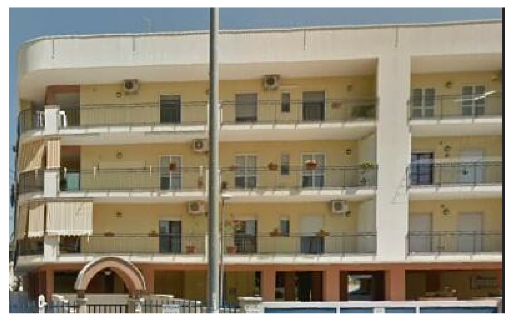
• Evaluation parameters: Most of the image data sets available in literature are labelled with a single and specific label. This was not the underlying idea of View VULMA, considering that using a single label would result in an over-complicated, opinable and somehow fuzzy class label. Instead, we characterised each image in terms of different aspects, using a modular approach. The same image can be used for different scopes: As an example, an image representing a four-storey building with pilotis (Figure 1) can be used for training two networks, one for identifying the overall number of floors, and the other for detecting pilotis. To this end, 14 different parameters have been identified, making the data set able to be used in as many different independent classification tasks. A desirable side effect of this design choice is that the number of possible classes defined for each classification task is greatly reduced, and this can be seen as a way to mitigate the problem of the curse of dimensionality.
• Diversity: The third requirement of View VULMA consists in a feature of the overall data set, which should be characterised by enough intra- and inter-class variations. In other words, for each parameter, different labels should be properly described accounting for the variation of appearance, position, viewpoint and pose. Furthermore, images with occlusions and noise are not discarded, in order to improve the overall diversity provided by the data set and, at the same time, to train and test classification methods under challenging conditions.

3. Defining View VULMA

To define View VULMA according to requirements highlighted in Section 2, we envisioned an end-to-end development pipeline consisting of five main steps, as summarised in Figure 2.

3.1. Step 1: Candidates Collection

In the first step, candidate images are collected from some urban areas. The latter can be selected according to any kind of methods, but it could be interesting to act on areas characterised by buildings having similar typological features. Under this concept, a literature option is provided by CARTIS form [25], which provides a subdivision of the focused municipality in town compartments (TCs), as reduced areas having homogeneous building portfolios. Looking into these urban areas, View-VULMA can be characterised by an average of 500–1000 clean building images detected by Google Street View. Despite it being mandatory to collect a large amount of candidate images, this ambitious goal is often difficult to reach, considering some external factors that can affect the research, such as the number of roads and the effective buildings, for each TC. Anyway, the data collection starts with the conversion of a geographical representation of a specific TC from a shape format type (usually available from different data sources) into a GeoJSON format, which is specifically tailored to handle geographical information in a standardised fashion. This representation allows us to highlight all the roads contained in the TC, extracting information about embedded geographic locations in terms of latitude and longitude. Once this process has been performed, the building portfolio’s image collection can be carried out by looking within the focused TC through direct queries to Google Street View. Each query is performed by using the aforementioned locations provided by the GeoJSON file. In the end, to increase the number of images to gather, we fetched images taken at angles of 0, 90, 180 and 270 degrees with respect to the tangent of the considered street. This leads us to the step described in Section 3.1, where candidates are cleaned and organised.

3.2. Step 2: Candidate Cleaning

The previous step allows us to collect an extremely high number of images; however, there are two adversary effects to pay attention to:

• Replications, which are caused by a finer sampling of data points defined in step 1 if compared to images available on Google Street View;
• Non-meaningful data, which are caused by pictures gathered in rural areas, where buildings are not present, or where these are completely obstructed by roads or trees.

The first issue has been handled by performing a specific cleaning procedure based on the digest of the information contained into each picture. Remembering that a hash function is a non-invertible function, the output is represented by a specific value (i.e., the digest) for a given input. The main characteristic of a hash function is that it is extremely unlikely that two inputs will give the same digest as the output of the function. Therefore, if for a pair of images $(i,j)$ holds the following:

$$h\left(i\right)=h\left(j\right)$$

(1)

where $h\left(i\right)$ is the digest of i, and $h\left(j\right)$ is the digest of j, it is likely that i = j, and hence one of the images in the pair can be discarded. This approach is computationally effective and has been preferred to an extremely computationally intensive pixel-by-pixel comparison between the two images. The issue of non-meaningfulness of (some) data has been directly handled as described in the following step.

3.3. Step 3: Candidates Selection

In the third step, domain experts have been involved to identify whether a candidate should be retained or discarded as non-meaningful. Specifically, the following criteria have been used to identify non-meaningful images:

• No buildings are available in the image;
• Buildings are available, but their overall relevance was below $20\%$. In other words, this means that both the width and the height of the region of interest (i.e., the building) are represented by less than $128\times 128$ pixels, therefore yielding an inadequate resolution for proper processing. Obviously, this is an empirical threshold and can be refined in future revisions of View VULMA.

The entire process has been performed manually for the entire dataset, mainly due to the lack of specifically trained models. However, the burden on domain experts has been lowered by the candidate cleaning performed in step 2.

3.4. Step 4: Candidate Labelling

In step 4, domain experts have been once again involved to label the outcomes of step 3. In particular, the resultant number of available images at this point amounted to about $20.000$ (as extracted by the 5 TCs), with an average of $4.000$ images per TC. Hence, domain experts performed labelling according to 14 different typological parameters, each of which has been denoted as $V_j$, where $j\in [1,14]$. Each typological parameter can be labelled through some possible values, such as described in

Table 1. Labels provided in View VULMA. The symbols $n_u$, $n_s$ and $n_o$ indicate the maximum numbers of units, storeys and openings observable in the entire image, respectively. Obviously, there is not a fixed maximum, which can be updated by increasing the data set.

Typological Parameters—Labels	Values
Structural typology	Reinforced concrete/Masonry
Number of units	$[1,\dots ,n_u]$
Number of storeys	$[1,\dots ,n_s]$
Presence of pilotis floor	True/False
Presence of basement floor	True/false
Presence of superelevation floor	True/false
Total number of openings	$[0,\dots ,n_o]$
Type of roof floor	Dome/Flap/Plan/Not Displayed
Presence of vaults	True/False
Presence of visible seismic details	True/False
Presence of higher ground floor	True/false
Presence of overhangs	True/False
Regularity in-plan	True/False
Regularity in-height	True/False

.

It is important to underline that each image has been reviewed by at least two domain experts. Given the even number of experts, a weighted consensus procedure has been followed. Specifically, we started presenting a junior researcher with a set of candidate images, and a form containing all $V_j$ and the related values to be filled. We then asked the researcher to fill the aforementioned forms, encouraging him/her to select labels regardless of occlusions, noise, background clutter and other adversarial effects. This was a precise design choice to improve diversity (see Section 2). After the junior researcher completed his/her work, a senior researcher reviewed the work of the junior researcher, possibly giving another interpretation on the labelling. To avoid conflicts, the weighted consensus automatically assigned a higher score to the senior researcher, therefore guaranteeing him/her a final word on the choice of each label for each parameter. After the weighted consensus procedure, the candidate is considered as labelled, and it is ready to be used for supervised classification tasks.

3.5. Step 5: Candidate Balancing

The main issue characterising the output given by the step in Section 3.4 is a possible unbalancing, properly observing the number of images of each $V_j$. In particular, if the focused parameters presents a value, e.g., presence of pilotis—Yes/No, which is not present in $80\%$ of the images and is present in the remaining $20\%$, the data set is not balanced for that parameter. To overcome the possibility that the data may not be uniformly distributed among possible values, a balancing step has been predisposed, as characterised by a twofold procedure.

• Data augmentation: The importance of data augmentation in deep learning has been extensively described [26]. Hence, data are augmented by using an automatic script which fetches from the Internet images related to the undersampled terms. As an example, if the data set is heavily skewed in terms of pictures presenting the pilotis plane (to use the previous example), the tool will select images relative to terms such as pilotis plane, presence of pilotis and so on, in different languages (e.g., Italian, Spanish, English). We recognise the semantic power of this tool is yet to be improved due to the extremely specific combination of words to be used for each case, and several improvements can be performed.
• Hard negative mining: If the data augmentation procedure is not sufficient to make the uniformly distributed for the considered $V_j$, hard negative mining is performed by randomly subsampling images labelled with the most represented parameter. In our example, the set of images that does not show the pilotis plane will be subsampled, with a randomly dropped action on the set of images.

Algorithm 1 briefly outlines the candidates balancing procedure followed during the definition of View VULMA.

Algorithm 1 Pseudo-code for View VULMA data balancing.

Require:  $V_j=[v_0,\dots ,v_k]$ Require:  $m\in [0,k],n\in [0,k],m\ne n$ Ensure:  $P(X,v_m)=P(X,v_n)$ 1: Let $V_j=[v_0,v_k]$, X 2: for all$(m,n)$do 3:     while $P\left(v_m\right)\ne P\left(v_n\right)$ do 4:         Augment(X) 5:         if $\mathbf{then}P\left(v_m\right)>P\left(v_n\right)$ 6:            Undersample($X\left(v_m\right)$) 7:         else 8:            Undersample($X\left(v_n\right)$) 9:         end if 10:     end while 11: end for

Specifically, it is supposed that initially X images for the jth parameter $V_j$, whose values is in the set of values $[v_0,\dots ,v_k]$, are available. The final goal is to ensure that, for each pair of labels m and n, the probability that a sample labelled with m is equal to the probability to draw a sample labelled with n. In other words:

$$P\left(v_m\right)=P\left(v_n\right)$$

(2)

Hence, we use a dividi-et-impera (divide and conquer) approach by dividing the overall problem in a series of simpler problems, each one of which deals with balancing only two labels. Hence, we first perform data augmentation to avoid having to deal with the curse of dimensionality; afterwards, we undersample the most probable label by performing the procedure again if needed. Herein, we are not explicitly defining an undersampling algorithm on purpose.

4. Applications and Availability of View VULMA

View VULMA has been used in [21] as a basis for creating one of the modules by which the VULMA toolset is composed, specifically Bi VULMA. In the paper, it is shown that, despite the relatively small size of the early version of View VULMA used, optimal results can be easily achieved on each parameter by using MobileNetV2 [27] and transfer learning [28]. Specifically, authors claim that an overall accuracy of $97\%$ in cross validation can be achieved by using ADAM [29] as the optimization algorithm and a standard cross-entropy loss function. In addition, Bi VULMA offers several other network base models for comparison, such as Xception [30], ResNet152v2, InceptionResNetV2 and MobileNetV2 [31,32].

From

Table 2. Comparison of CNNs models, in terms of loss and accuracy, using transfer learning (TL) and fine tuning (FT) on structural typology.

Base Model	Loss (%)		Accuracy (%)
	TL	FT	TL	FT
$VGG19$	0.3	0.06	86.6	97.66
$ResNet50V2$	0.12	0.03	94.89	98.77
$InceptionV3$	0.13	0.03	94.3	98.81
$MobileNetV2$	0.12	0.07	94.55	97.53
$DenseNet121$	0.16	0.06	93.79	97.66
$NasNetMobile$	0.17	0.06	92.55	97.62

,

Table 3. Comparison of CNNs models, in terms of loss and accuracy, using transfer learning (TL) and fine tuning (FT) on number of units typology.

Base Model	Loss (%)		Accuracy (%)
	TL	FT	TL	FT
$VGG19$	0.18	0.12	94.96	96.41
$ResNet50V2$	0.12	0.05	95.99	98.29
$InceptionV3$	0.15	0.04	95.01	98.55
$MobileNetV2$	0.14	0.08	95.18	96.8
$DenseNet121$	0.16	0.1	95.22	96.76
$NasNetMobile$	0.17	0.09	94.92	96.67

,

Table 4. Comparison of CNNs models, in terms of loss and accuracy, using transfer learning (TL) and fine tuning (FT) on number of storeys.

Base Model	Loss (%)		Accuracy (%)
	TL	FT	TL	FT
$VGG19$	1.21	0.54	48.48	80.12
$ResNet50V2$	0.66	0.29	72.91	88.71
$InceptionV3$	0.87	0.28	63.33	89.66
$MobileNetV2$	0.79	0.5	68.31	80.65
$DenseNet121$	0.94	0.51	60.01	80.36
$NasNetMobile$	0.96	0.59	58.82	75.76

,

Table 5. Comparison of CNNs models, in terms of loss and accuracy, using transfer learning (TL) and fine tuning (FT) on presence of pilotis floor.

Base Model	Loss (%)		Accuracy (%)
	TL	FT	TL	FT
$VGG19$	0.11	0.03	97.41	98.94
$ResNet50V2$	0.05	0.02	98.13	99.49
$InceptionV3$	0.07	0.01	97.66	99.7
$MobileNetV2$	0.05	0.03	97.83	99.02
$DenseNet121$	0.07	0.03	97.53	99.06
$NasNetMobile$	0.07	0.02	97.58	99.15

,

Table 6. Comparison of CNNs models, in terms of loss and accuracy, using transfer learning (TL) and fine tuning (FT) on presence of basement floor.

Base Model	Loss (%)		Accuracy (%)
	TL	FT	TL	FT
$VGG19$	0.21	0.13	94.26	94.98
$ResNet50V2$	0.16	0.06	94.52	97.79
$InceptionV3$	0.18	0.05	94.35	98.13
$MobileNetV2$	0.17	0.09	94.64	96.34
$DenseNet121$	0.18	0.1	94.39	96.22
$NasNetMobile$	0.18	0.12	94.3	95.58

,

Table 7. Comparison of CNNs models, in terms of loss and accuracy, using transfer learning (TL) and fine tuning (FT) on presence of superelevation floor.

Base Model	Loss (%)		Accuracy (%)
	TL	FT	TL	FT
$VGG19$	0.01	0.01	99.83	99.83
$ResNet50V2$	0.0	0.0	99.83	99.91
$InceptionV3$	0.01	0.0	99.83	100.0
$MobileNetV2$	0.01	0.0	99.83	99.96
$DenseNet121$	0.01	0.01	99.83	99.83
$NasNetMobile$	0.01	0.0	99.83	99.91

,

Table 8. Comparison of CNNs models, in terms of loss and accuracy, using transfer learning (TL) and fine tuning (FT) on total number of openings.

Base Model	Loss (%)		Accuracy (%)
	TL	FT	TL	FT
$VGG19$	2.58	1.72	19.9	44.18
$ResNet50V2$	1.44	0.79	51.4	73.0
$InceptionV3$	2.02	0.91	33.84	69.69
$MobileNetV2$	1.77	1.34	42.05	57.19
$DenseNet121$	2.15	1.6	30.91	47.53
$NasNetMobile$	2.17	1.66	29.76	46.73

,

Table 9. Comparison of CNNs models, in terms of loss and accuracy, using transfer learning (TL) and fine tuning (FT) on type of roof floor.

Base Model	Loss (%)		Accuracy (%)
	TL	FT	TL	FT
$VGG19$	0.55	0.31	75.37	86.99
$ResNet50V2$	0.42	0.22	81.3	91.14
$InceptionV3$	0.45	0.2	79.62	91.42
$MobileNetV2$	0.44	0.34	80.46	85.63
$DenseNet121$	0.25	0.32	88.09	86.61
$NasNetMobile$	0.47	0.32	79.71	86.47

,

Table 10. Comparison of CNNs models, in terms of loss and accuracy, using transfer learning (TL) and fine tuning (FT) on presence of vaults.

Base Model	Loss (%)		Accuracy (%)
	TL	FT	TL	FT
$VGG19$	0.31	0.15	85.1	92.99
$ResNet50V2$	0.21	0.08	89.68	96.54
$InceptionV3$	0.23	0.07	89.4	96.78
$MobileNetV2$	0.23	0.15	89.12	92.25
$DenseNet121$	0.47	0.13	79.85	93.51
$NasNetMobile$	0.27	0.15	86.5	92.67

,

Table 11. Comparison of CNNs models, in terms of loss and accuracy, using transfer learning (TL) and fine tuning (FT) on presence of visible seismic details.

Base Model	Loss (%)		Accuracy (%)
	TL	FT	TL	FT
$VGG19$	0.04	0.03	98.42	98.77
$ResNet50V2$	0.03	0.02	98.93	99.12
$InceptionV3$	0.02	0.01	99.02	99.42
$MobileNetV2$	0.03	0.01	99.42	99.63
$DenseNet121$	0.02	0.01	99.48	99.62
$NasNetMobile$	0.01	0.01	98.97	99.07

,

Table 12. Comparison of CNNs models, in terms of loss and accuracy, using transfer learning (TL) and fine tuning (FT) on presence of higher ground floor.

Base Model	Loss (%)		Accuracy (%)
	TL	FT	TL	FT
$VGG19$	0.07	0.02	98.6	99.44
$ResNet50V2$	0.03	0.01	98.84	99.86
$InceptionV3$	0.04	0.0	98.65	99.91
$MobileNetV2$	0.04	0.01	98.84	99.67
$DenseNet121$	0.05	0.03	98.65	99.21
$NasNetMobile$	0.05	0.02	98.6	99.3

,

Table 13. Comparison of CNNs models, in terms of loss and accuracy, using transfer learning (TL) and fine tuning (FT) on presence of overhangs.

Base Model	Loss (%)		Accuracy (%)
	TL	FT	TL	FT
$VGG19$	0.47	0.17	77.6	93.4
$ResNet50V2$	0.35	0.1	85.2	96.13
$InceptionV3$	0.37	0.08	83.03	96.98
$MobileNetV2$	0.35	0.2	83.59	92.46
$DenseNet121$	0.39	0.18	81.0	92.88
$NasNetMobile$	0.41	0.22	81.05	90.95

,

Table 14. Comparison of CNNs models, in terms of loss and accuracy, using transfer learning (TL) and fine tuning (FT) on regularity in plan.

Base Model	Loss (%)		Accuracy (%)
	TL	FT	TL	FT
$VGG19$	0.38	0.22	86.04	90.99
$ResNet50V2$	0.3	0.12	87.74	95.9
$InceptionV3$	0.33	0.1	86.32	96.13
$MobileNetV2$	0.32	0.22	86.46	90.85
$DenseNet121$	0.36	0.22	85.71	91.18
$NasNetMobile$	0.35	0.23	86.13	91.04

and

Table 15. Comparison of CNNs models, in terms of loss and accuracy, using transfer learning (TL) and fine tuning (FT) on regularity in height.

Base Model	Loss (%)		Accuracy (%)
	TL	FT	TL	FT
$VGG19$	0.26	0.16	92.02	94.44
$ResNet50V2$	0.21	0.08	92.61	97.17
$InceptionV3$	0.22	0.05	92.57	98.04
$MobileNetV2$	0.22	0.14	92.75	94.66
$DenseNet121$	0.23	0.14	92.57	94.94
$NasNetMobile$	0.24	0.14	92.11	94.57

, the comparison among six models of CNNs, specifically VGG19 [33], ResNet50v2, InceptionV3, MobileNetV2, DenseNet [34,35] and NasNetMobile, is shown for each parameter. This comparison has been carried out using mainly Bi VULMA but alsi including a specific integration for VGG19 and DenseNet, which are not currently available within the tool. It is worth noting that the selection of the CNNs models is not casual and it has been made according to two main principles: (i) They are the most recent models developed and available in the scientific literature; (ii) they have been selected according to the possible hardware at disposal to the authors, also considering the best performances available for these kinds of applications. As for results, in all Tables, both the loss and accuracy are shown for transfer learning (20 epochs) and fine tuning (10 epochs) with a learning rate of 0.001. Each base model has been pre-trained on ImageNet, and a standard train/validation/test ratio of 70/20/10 has been selected over each topological parameter. The tests took two days to be performed on an NVIDIA GeForce 3070 RTX with 10 GBs of RAM. As expected, fine tuning the entire model after a round of transfer learning further improves accuracy results, even in the most challenging problems, which are the classification of the total number of storeys and the classification of the total number of openings. Specifically, these parameters are challenging mainly due to the high number of possible classes, and probably require more data with respect to the other parameters. It is also interesting to underline how both ResNet and Inception outperform other models in almost any situation, hence further exploration of these architectures along with their successors may be required as the View VULMA grows.

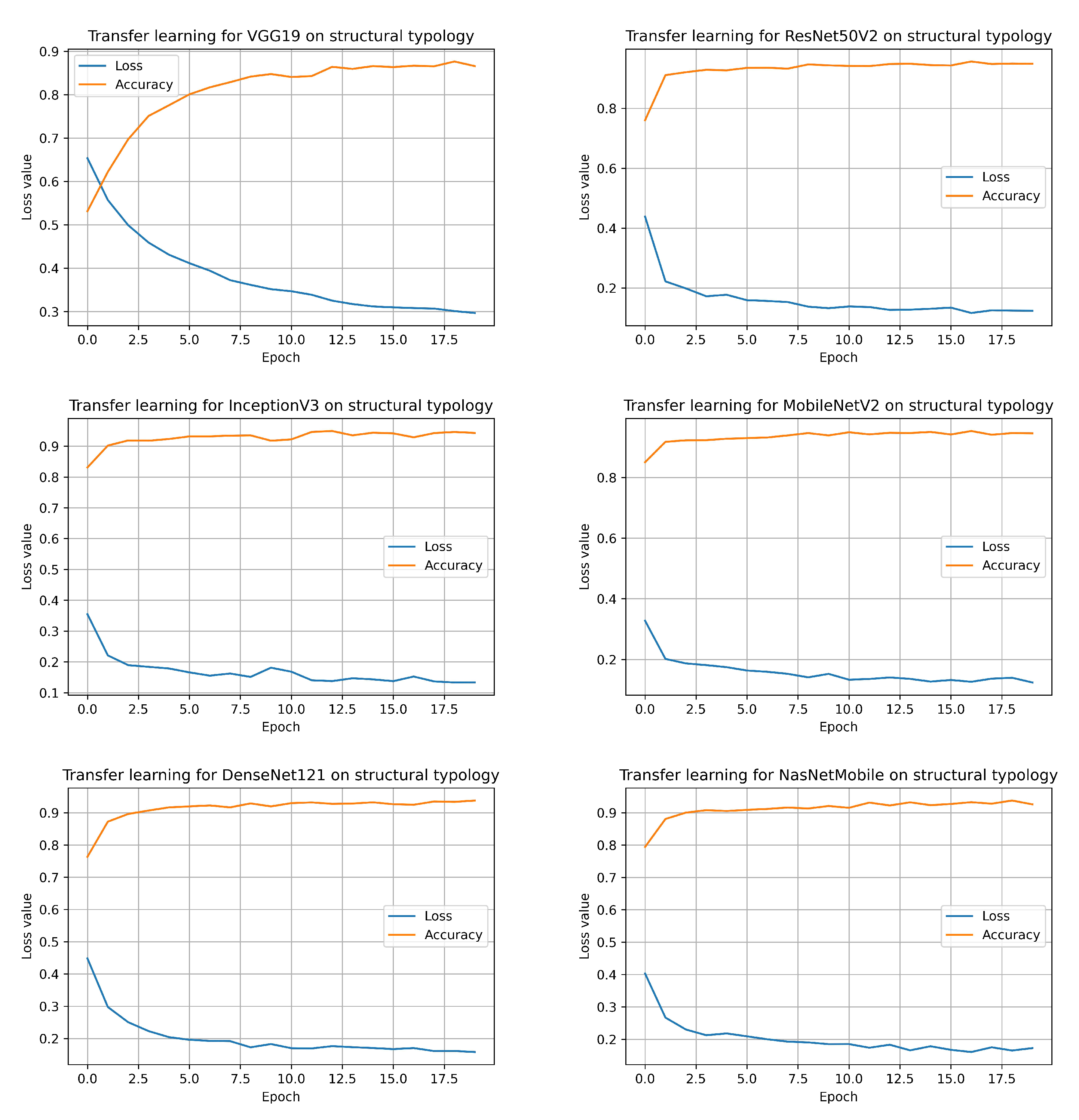
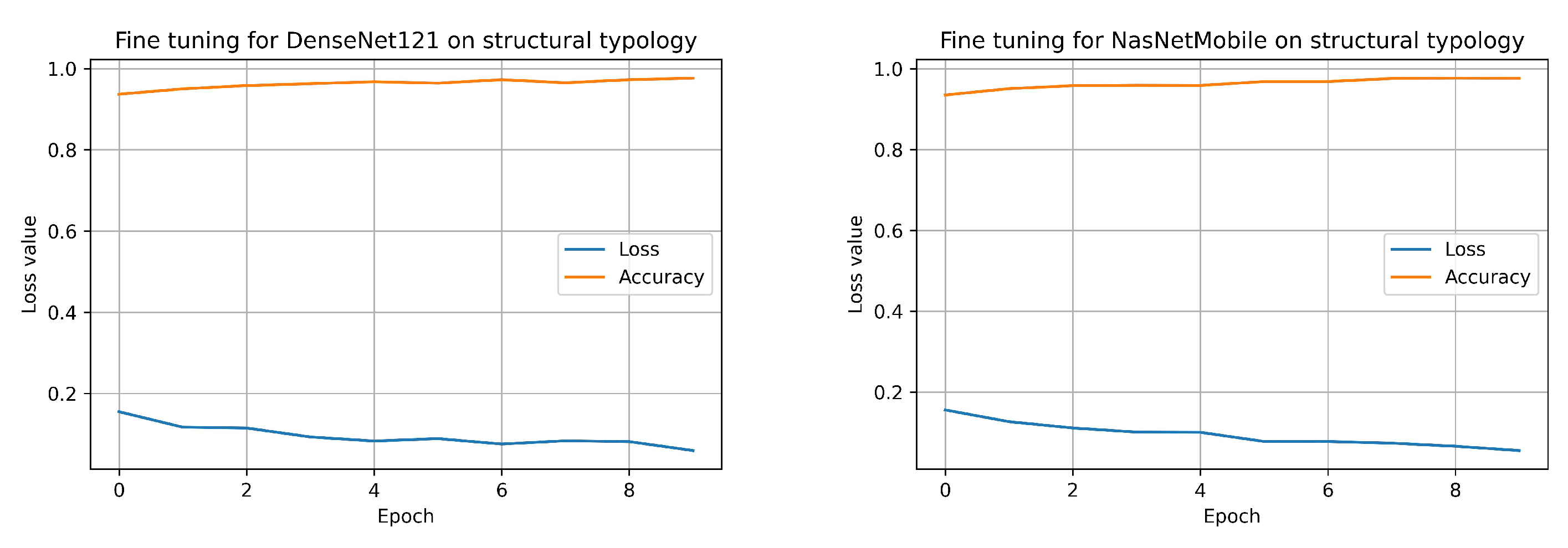
Still, only for the parameter structural typology, the graphs about the training for all employed CNNs models are reported, showing the trends of both loss and accuracy for transfer learning (Figure 3) and fine tuning (Figure 4) phases.

In the end, it is important to underline that transfer learning has been preferred as the quantity of data available in View VULMA is still limited. However, results are promising, and show the potential of using this for developing an end-to-end ML tool for seismic assessment. As for its availability, we plan to publicly distribute View VULMA as soon as possible; as already stated in Section 2, our goal is to incorporate at least $50.000$ images of different buildings before it is made available to a wider audience. However, interested researchers can contact the corresponding author to receive a preliminary version of the data set.

5. Conclusions

Currently, View VULMA constitutes only a restricted data set, which for making reliable a tool such as VULMA needs to be strongly improved, accounting for other typological parameters (e.g., steel and precasted buildings). Still, the improvements of the data set could be used to identify other sources of vulnerability, such as structural and non-structural elements decay. To further speed up the construction process of the data set, we will continue to explore more effective methods to evaluate user labels, by optimising the number of needful repetitions to accurately assess each image. In summary, to complete View VULMA, it is necessary: (1) to increase the number of labelled images and the number of parameters to label; (2) to deliver View VULMA to the research community directly by making it publicly available and readily accessible online; (3) to promote View VULMA through an online platform where everyone can contribute to increase the data samples and, at the same time, to benefit from View VULMA as a resource. In the end, View VULMA and in a particular way, VULMA, could become a central resource for a broad range of vision-based seismic vulnerability assessment research.

References

1. GNDT Gruppo Nazionale Per la Difesa dai Terremoti. Rischio Sismico di Edifici Pubblici; GNDT Gruppo Nazionale Per la Difesa dai Terremoti: Roma, Italy, 1993; pp. 1–134. (In Italian) [Google Scholar]
2. Baggio, C.; Bernardini, A.; Colozza, R.; Corazza, L.; Della Bella, M.; Di Pasquale, G.; Zuccaro, G. Field Manual for Post-Earthquake Damage and Safety Assessment and Short Term Countermeasures (AeDES); European Commission—Joint Research Centre—Institute for the Protection and Security of the Citizen: Ispra, Italy, 2007; p. 22868. [Google Scholar]
3. Dolce, M.; Speranza, E.; Giordano, F.; Borzi, B.; Bocchi, F.; Conte, C.; Di Meo, A.; Faravelli, M.; Pascale, V. Observed damage database of past Italian earthquakes: The Da. DO WebGIS. Boll. Geofis. Teor. Appl. 2019, 60, 141–164. [Google Scholar] [CrossRef]
4. Nicodemo, G.; Pittore, M.; Masi, A.; Manfredi, V. Modelling exposure and vulnerability from post-earthquake survey data with risk-oriented taxonomies: AeDES form, GEM taxonomy and EMS-98 typologies. Int. J. Disaster Risk Reduct. 2020, 50, 101894. [Google Scholar] [CrossRef]
5. Del Gaudio, C.; Di Ludovico, M.; Polese, M.; Manfredi, G.; Prota, A.; Ricci, P.; Verderame, G.M. Seismic fragility for Italian RC buildings based on damage data of the last 50 years. Bull. Earthq. Eng. 2020, 18, 2023–2059. [Google Scholar] [CrossRef]
6. Rosti, A.; Del Gaudio, C.; Rota, M.; Ricci, P.; Di Ludovico, M.; Penna, A.; Verderame, G.M. Empirical fragility curves for Italian residential RC buildings. Bull. Earthq. Eng. 2020, 19, 3165–3183. [Google Scholar] [CrossRef]
7. Ruggieri, S.; Tosto, C.; Perrone, D.; Uva, G.; Aiello, M.A. Assessment of post-earthquake damages on Italian school building portfolios over the last 50 years. In Proceedings of the COMPDYN 2021, 8th ECCOMAS Thematic Conference on Computational Methods in Structural Dynamics and Earthquake Engineering, Athens, Greece, 27–30 June 2021. [Google Scholar]
8. Ruggieri, S.; Tosto, C.; Rosati, G.; Uva, G.; Ferro, G.A. Seismic vulnerability analysis of Masonry Churches in Piemonte after 2003 Valle Scrivia earthquake: Post-event screening and situation 17 years later. Int. J. Archit. Herit. 2020. [Google Scholar] [CrossRef]
9. De Matteis, G.; Brando, G.; Corlito, V. Predictive model for seismic vulnerability assessment of churches based on the 2009 L’Aquila earthquake. Bull. Earthq. Eng. 2019, 17, 4909–4936. [Google Scholar] [CrossRef]
10. Leggieri, V.; Ruggieri, S.; Zagari, G.; Uva, G. Appraising seismic vulnerability of masonry aggregates through an automated mechanical-typological approach. Autom. Constr. 2021, 132, 103972. [Google Scholar] [CrossRef]
11. Ruggieri, S.; Porco, F.; Uva, G.; Vamvatsikos, D. Two frugal options to assess class fragility and seismic safety for low-rise reinforced concrete school buildings in Southern Italy. Bull. Earthq. Eng. 2021, 19, 1415–1439. [Google Scholar] [CrossRef]
12. Donà, M.; Carpanese, P.; Follador, V.; Sbrogiò, L.; da Porto, F. Mechanics-based fragility curves for Italian residential URM buildings. Bull. Earthq. Eng. 2020, 19, 3099–3127. [Google Scholar] [CrossRef]
13. Ruggieri, S.; Perrone, D.; Leone, M.; Uva, G.; Aiello, M.A. A prioritization RVS methodology for the seismic risk assessment of RC school buildings. Int. J. Disaster Risk Reduct. 2020, 51, 101807. [Google Scholar] [CrossRef]
14. Xie, Y.; Sichani, M.E.; Padgett, J.E.; DesRoches, R. The promise of implementing machine learning in earthquake engineering: A state-of-the-art review. Earthq. Spectra 2020, 36, 1769–1801. [Google Scholar] [CrossRef]
15. Xu, Y.J.; Lu, X.; Huang, Y.L. Real-time seismic damage prediction and comparison of various ground motion intensity measures based on machine learning. J. Earthq. Eng. 2020, 24, 1–21. [Google Scholar] [CrossRef]
16. Ferreira, T.M.; Estevao, J.; Maio, R.; Vicente, R. The use of artificial neural networks to estimate seismic damage and derive vulnerability functions for traditional masonry. Front. Struct. Civ. Eng. 2020, 14, 609–622. [Google Scholar] [CrossRef]
17. Harirchian, E.; Lahmer, T.; Rasulzade, S. Earthquake hazard safety assessment of existing buildings using optimized multi-layer perceptron neural network. Energies 2020, 13, 2060. [Google Scholar] [CrossRef] [Green Version]
18. Harirchian, E.; Jadhav, K.; Kumari, V.; Lahmer, V. ML-EHSAPP: A prototype for machine learning-based earthquake hazard safety assessment of structures by using a smartphone app. Eur. J. Environ. Civ. Eng. 2021, 1–21. [Google Scholar] [CrossRef]
19. Mangalathu, S.; Sun, H.; Nweke, C.C.; Yi, Z.; Burton, H.V. Classifying earthquake damage to buildings using machine learning. Earthq. Spectra 2020, 36, 183–208. [Google Scholar] [CrossRef]
20. Mangalathu, S.; Hwang, S.H.; Choi, E.; Jeon, J.S. Rapid seismic damage evaluation of bridge portfolios using machine learning techniques. Eng. Struct. 2019, 201, 109785. [Google Scholar] [CrossRef]
21. Ruggieri, S.; Cardellicchio, A.; Leggieri, V.; Uva, G. Machine-learning based vulnerability analysis of existing buildings. Autom. Constr. 2021, 132, 103936. [Google Scholar] [CrossRef]
22. Available online: https://github.com/Project-VULMA (accessed on 31 October 2021).
23. Albawi, S.; Mohammed, T.A.; Al-Zawi, S. Understanding of a convolutional neural network. In Proceedings of the 2017 International Conference on Engineering and Technology (ICET), Antalya, Turkey, 21–23 August 2017; pp. 1–6. [Google Scholar]
24. Frassine, L.; Giovinazzi, S. Basi di dati a confronto nell’analisi di vulnerabilità sismica dell’edilizia residenziale: Un’applicazione per la città di Catania. In Proceedings of the XI Congresso Nazionale “L’ingegneria Sismica in Italia”, Genova, Italy, 25–29 January 2004; p. 16. (In Italian). [Google Scholar]
25. Zuccaro, G.; Dolce, M.; De Gregorio, D.; Speranza, D.; Moroni, C. La Scheda Cartis Per La Caratterizzazione Tipologico—Strutturale Dei Comparti Urbani Costituiti Da Edifici Ordinari. Valutazione dell’esposizione in analisi di rischio sismico. Proc. GNGTS 2015, 281–287. Available online: http://www3.ogs.trieste.it/gngts/files/2015/S23/Riassunti/Zuccaro.pdf (accessed on 31 October 2021).
26. Shorten, C.; Khoshgoftaar, T.M. A survey on image data augmentation for deep learning. J. Big Data 2019, 6, 1–48. [Google Scholar] [CrossRef]
27. Sandler, M.; Howard, A.; Zhu, M.; Zhmoginov, A.; Chen, L.C. Mobilenetv2: Inverted residuals and linear bottlenecks. In Proceedings of the IEEE Conference on Computer Vision and Pattern Recognition, Salt Lake City, UT, USA, 19–23 June 2018; pp. 4510–4520. [Google Scholar]
28. Torrey, L.; Shavlik, J. Transfer learning. In Handbook of Research on Machine Learning Applications and Trends: Algorithms, Methods, and Techniques; IGI Global: Hershey, PA, USA, 2010; pp. 242–264. [Google Scholar]
29. Kingma, D.P.; Ba, J. Adam: A method for stochastic optimization. arXiv 2014, arXiv:1412.6980. [Google Scholar]
30. Chollet, F. Xception: Deep learning with depthwise separable convolutions. In Proceedings of the IEEE Conference on Computer Vision and Pattern Recognition, Honolulu, HI, USA, 21–26 July 2017; pp. 1251–1258. [Google Scholar]
31. He, K.; Zhang, X.; Ren, S.; Sun, J. Identity mappings in deep residual networks. In European Conference on Computer Vision; Springer: Cham, Switzerland, 2016; pp. 630–645. [Google Scholar]
32. Szegedy, C.; Vanhoucke, V.; Ioffe, S.; Shlens, J.; Wojna, Z. Rethinking the inception architecture for computer vision. In Proceedings of the IEEE Conference on Computer Vision and Pattern Recognition, Las Vegas, NV, USA, 27–30 June 2016; pp. 2818–2826. [Google Scholar]
33. Simonyan, K.; Zisserman, A. Very deep convolutional networks for large-scale image recognition. arXiv 2014, arXiv:1409.1556. [Google Scholar]
34. Zoph, B.; Vasudevan, V.; Shlens, J.; Le, Q.V. Learning transferable architectures for scalable image recognition. In Proceedings of the IEEE Conference on Computer Vision and Pattern Recognition, Salt Lake City, UT, USA, 18–23 June 2018; pp. 8697–8710. [Google Scholar]
35. Huang, G.; Liu, Z.; Van Der Maaten, L.; Weinberger, K.Q. Densely connected convolutional networks. In Proceedings of the IEEE Conference on Computer Vision and Pattern Recognition, Honolulu, HI, USA, 21–26 July 2017; pp. 4700–4708. [Google Scholar]
Figure 1. Example of photo used in View VULMA, from which it extracts the number of floors and presence of pilotis. It is worth noting that the occlusion, the light pole, does not represent an issue for the next steps.
Data 07 00004 g001
Figure 2. Logic scheme of steps involved in the definition of View VULMA.
Data 07 00004 g002
Figure 3. Transfer learning for VGG19, ResNet50v2, InceptionV3, MobileNetV2, DenseNet and NasNetMobile on structural typology.
Data 07 00004 g003
Figure 4. Fine tuning for VGG19, ResNet50v2, InceptionV3, MobileNetV2, DenseNet and NasNetMobile on structural typology.
Data 07 00004 g004aData 07 00004 g004b