Data Descriptor

Short Baseline Observations at Geodetic Observatory Wettzell

Geodetic Observatory Wettzell, Federal Agency for Cartography and Geodesy, Sackenrieder Str. 25, 93444 Bad Koetzting, Germany
*
Author to whom correspondence should be addressed.
Submission received: 15 November 2018 / Revised: 23 November 2018 / Accepted: 25 November 2018 / Published: 10 December 2018
(This article belongs to the Special Issue Data in Astrophysics & Geophysics: Research and Applications)

Abstract

:
The Geodetic Observatory Wettzell (GOW), jointly operated by the Federal Agency for Cartography and Geodesy (BKG), Germany and the Technical University of Munich, Germany is equipped with three radio telescopes for Very Long Baseline Interferometry (VLBI). Correlation capability is primarily designed for relative positioning of the three Wettzell radio telescopes i.e., to derive the local ties between the three telescopes from VLBI raw data in addition to the conventional terrestrial surveys. A computing cluster forming the GO Wettzell Local Correlator (GOWL) was installed in 2017 as well as the Distributed FX (DiFX) software correlation package and the Haystack Observatory Postprocessing System (HOPS) for fringe fitting and postprocessing of the output. Data pre-processing includes ambiguity resolution (if necessary) as well as the generation of the geodetic database and NGS card files with υ Solve. The final analysis is either carried out with local processing software (LEVIKA short baseline analysis) or with the Vienna VLBI and Satellite (VieVS) software. We will present an overview of the scheduling, correlation and analysis capabilities at GOW and results obtained so. The dataset includes auxiliary files (schedule and log files) which contain information about the participating antenna, observed sources, clock offset between formatter and GPS time, cable delay, meteorological parameters (temperature, barometric pressure, and relative humidity) and ASCII files created after fringe fitting and final analysis. The published dataset can be used by the researchers and scientists to further explore short baseline interferometry.
Dataset License: CC BY 4.0

1. Summary

This paper is intended to give the readers an insight into all the stages of data processing before and after a VLBI experiment. VLBI is a technique which is based on the computation of the time delay in the arrival of a radio frequency signal transmitted by a remote astronomical source (generally a quasar) between radio telescopes. At GOW, since 2017 two sibling VLBI telescopes (shown in Figure 1) which are 123 metre apart are used to make short baseline observations. The main idea of making such observations is to understand the difference between long and short baseline observations in terms of estimated parameters due to common troposphere and ionosphere and compare it with the results of local survey measurements [1]. Local sessions with short duration are also scheduled predominantly for research and development work conducted on the regular basis. These sessions are helpful in terms of quality affirmation at the VLBI sites and can provide quick feedback about the health of the system. To start planning any kind of local session whether experimental or geodetic it is very important to find common timeslots where both the telescopes are not participating in any of the long baseline observations. The VLBI telescopes at Wettzell [2] are currently participating in different types of sessions which are proposed by IVS [3] and to make this job easy a coordination tool [4] is developed. The coordination tool is useful for planning, coordinating, keeping track of the status of the session and statistical analysis. The principal investigator (P.I.) has to submit a request for the local session based on the available time interval for the baselines of interest using the tool.
Table 1 provides statistics about all the different types of sessions observed in the year of 2017 by the two VLBI (legacy mode) telescopes from the GOW. Table 2 gives information about the technical specifications in terms of hardware installed at the telescopes [5,6]. Raw data from all the participating telescopes are sent to the correlation center either by an internet link or by shipping the hard disks. The correlation center is responsible for correlating and fringe fitting the observed data. A software correlator called DiFX [7,8] is currently used by most of the correlation centres around the globe. The fringe fitting software accounts for insufficiencies in the correlator model and integrates the interferometer signal. The software package called HOPS [9] is used for fringe fitting the correlated data. Fringe plots are helpful in detecting problems at the station and checking the quality of the data. A fringe plot is a collection of multiple plots on a page along with written information about a single scan. A description of the fringe plot for the analyst is given in Section 3.4. The fringe fitted data are further analysed in the postprocessing software for ambiguity resolution and ionospheric correction. The results are written in an ASCII file containing group delay information corresponding to each scan which is read by the in-house analysis software for the estimation of geodetic parameters, e.g., baseline vector and clock drift. The published dataset contains sessions observed with telescopes connected to separate clocks.

2. Data Description

The published dataset includes sessions observed in the year 2017 and 2018. From scheduling to analysis [10] all the different data types and file formats used in the VLBI processing will be described in this section. Scheduling is defined as the observation plan for the participating telescopes i.e., list of all the observed sources, source and station positions, observation epoch, duration of individual scans and additional information related to hardware. Two commonly used software (sked [11,12] and VieVS [13]) are installed for scheduling local (both long and short baseline) sessions. All the details about the file types are given in Section 2.1. VLBI measurement [14] takes place after the schedule is provided to all the network stations. The operators at each site use field system [15] to communicate with the hardware (mainly data acquisition system). To keep track of observation, field system generates log files where system check commands together with the operator comments are stored. Section 2.2 is dedicated to providing a brief overview of the useful information written in the log files during the measurement. The recorded raw data and the log files are transferred to the correlator facility. Further information related to the file formats generated at this step of data processing can be found in Section 2.3. The fringe fitted data are the input to the VLBI analysis software [16] developed for geodetic parameter estimation (EOP [17] and station coordinates [18] in particular). In Section 2.4 and Section 2.5 descriptions of the NetCDF and ASCII files generated during the analysis process is given respectively.

2.1. Schedule Files

The Vienna VLBI and Satellite Software (VieVS) [19] is used for scheduling local sessions. For generating a schedule file, start time and duration of the requested session has to be inserted in addition to the list of participating stations. Two files are created as an output after providing all the required input information to the scheduling software i.e., sessionname.skd and sessionname.vex file.

2.1.1. Skd File

The schedule files with the extension .skd are mainly generated for the VLBI measurement purpose. These files are read by ’drudg’ subroutine for producing snap and procedure files as an output for individual participating telescopes. A brief description of all the sections present in the .skd file is given in Table 3. A detailed description of all the sections in a .skd file can be found in [20]. Procedure file contains information related to the hardware configuration, e.g., type of back-end, number of channels, bit-rate, local oscillator frequencies and other details, for instance, phase-Cal unit, baseband frequency with bandwidth and polarization. Snap file provides information about the position of the source at the time of observation for each network station allowing the antenna control unit to point in the right direction.

2.1.2. VEX File

The VEX stands for VLBI Experiment. The .vex file [21] is used for correlating the raw data after the session is observed. This file is either provided by the scheduler along with the .skd file to the correlation center or it is the responsibility of the correlation center to generate it. A vex file is a combination of snap and procedure file. Both source and hardware information essential for the correlation process is written in this file. It also contains frequency set-up and data recording rate set by the scheduler for a particular session. There are mainly three types of sections in a vex file. As shown in Figure 2, the blocks which are independently defined are in green. They are called primitive blocks. The high level blocks in pink are a combination of primitive-block keywords. The scheduling block in yellow contains a schedule for the measurement.

2.2. Log File

The scheduler has to send the schedule (.skd or .vex) file to all the participating stations where the operators create snap and procedure files in the Field System [22] (FS) using a program called ‘drudg’. Every single snap instruction by the operator with the feedback is recorded in a log file. The log files provide auxiliary information about the session and are used in the correlation and analysis stage of data processing. Operator’s comment section (Figure 3) also plays an important role in giving quick hint about the problems at the station to the data analyst.

2.2.1. Maser Offset

For estimation of precise value and rate of change of UT1, it is important for the data analyst to know the offset between 1 pulse per second generated by the maser at the station and the GPS 1 pulse per second signal. In addition to UT1 determination, this value is also necessary at the correlation stage in adjusting the fringe search window. Each VLBI site has its own timing system and for the sake of uniformity, it is mandatory to record the offset between the standard/reference with the station clock. The offset counter is connected to the field system computer for registering the offset at least one time per scan [23]. The offset is stored in the log file during the session either after ‘gps-fmout’ or ‘fmout-gps’ command depending on the cable connection to the counter.
These values are also important in detecting clock jumps at the station. Figure 4a is an example without clock jump whereas Figure 4b shows an example where WETTZELL telescope experienced clock jump during a 24-h VLBI session. All the scans in the red circle are observed after the clock jump and this has to be taken into consideration during the fringe search process.

2.2.2. Cable Delay

Cable delay system is installed for accounting the propagation delay caused by thermal or physical changes inside the VLBI system. Due to the presence of several electronic component inside the telescope, signal path monitoring plays an important role in estimating the instrumental delay [24]. Similar to clock offset, the calibration system is also connected to the field system computer and for each scan, a calibration signal is sent and received back. The values recorded by the cable delay system are written in the station log after ‘cable’ command. The cable delay values are used in the VLBI data analysis process. Cable delay values for WETTZELL station from the 18AUG02X9 session are shown in Figure 5.

2.2.3. Meteorological Data

For estimating additional delay caused by troposphere [25,26] during the wave propagation in the VLBI processing chain, it is important to record temperature, pressure and relative humidity values for each station during the observation for each scan. These values are stored in the station log after ’wx’ command and extracted by the analysis software for estimating tropospheric parameters (dry, wet delays and gradients). In the local sessions, the values for both the stations are recorded from the same meteorological sensor hence they are identical. In case of coordinate determination, short baseline observation shows more precise results as compared to long baseline observation. The main reason being, excess delay due to troposphere and ionosphere is close to negligible. Figure 6 shows recorded temperature, pressure and relative humidity values from session 18AUG02X9.

2.3. alist.out

Correlation and fringe fitting is performed at the correlation centre. The raw data are deleted after the analysis is finished to prevent disk space shortage. However, an ASCII file generated using HOPS [27] is stored for each correlated session. A file named alist.out contains scan-wise information about the session. This file is also used for creating a correlation report where session statistics is written with the correlation experts comment. List of important fields with the description in an alist.out is given in Table 4.

2.4. NetCDF/vgosDB

Database creation is the next step after the fringe fitting of the data. With the improvements in the technology and increasing demand, a new VLBI observation system called VGOS [28] is established. The main idea is to increase the observation type with broader bandwidth (2–14 GHz). So, to deal with data processing of VGOS style of observation [29], IVS working group 4 (WG4) [30] was established in 2007. Considering the fact that the amount of data will be high and it is important to have a file format which is easy to handle and know for the community, it was decided to use NetCDF as a standard file format. The fringe fitted output is input to the VLBI data analysis software [31] and the first database is generated which is NetCDF format. All the directories generated in the first database are listed with the description in Table 5. The data are split into pieces and stored in different folders to keep it flexible. A wrapper file is an ASCII file read by the software to locate specific data. They play a very important role in the whole data processing as they are never overwritten. It is very essential for testing different models and make comparisons. They also provide a lot of information and are stored with .wrp extension, e.g., 17SEP29X9_V001_kall.wrp where 17SEP29 is the session name, X9 is the session code and V001 is an indicator of version number which means, in this case, it is version 1.
Every time a session is processed, the version number incrementation takes place and a new wrapper file is created. The Head.nc file provides general information about the session, e.g., station list, source list and time of observation. Station folder contains station related information. Only two folders are available in case of this dataset i.e., WETTZELL and WETTZ13N. The start time of each scan can be found in Solve folder. Fourfit related information, e.g., control file and command string for each band are available in the sessions folder. Scan folder holds mainly all the information about the observed scan, e.g., scan names, a pointer to the fourfit output and observation time in UTC. The VLBI observables for each band are stored in the observables folder. A complete list with the description is available in Table 6.

2.5. NGS File

The most commonly used file format for legacy mode i.e., S and X band observation is NGS card [32]. It is mainly composed of an ASCII file with different cards based on the session and observation. Each file contains observables from a single band which means in case of dual band observation, two separate NGS card files are generated. The main objective of observing with dual frequency band is to remove propagation delay caused by the ionosphere. Short baseline measurements are never affected by this effect as both the telescopes are observing in the same part of the sky. Moreover, most of the scans in S-band are affected by RFI [33] mainly due to overlapping with Wi-Fi and telecommunication signal. This causes a hindrance in terms of assessing the data quality of the affected channels as they have to be flagged in the correlation process and are not contributing to further analysis. Hence, for short baseline measurements group delays only from X-band are used in the analysis process. The format of an NGS file [34] is described in Table 7.

3. Method

3.1. Schedule Preparation

The provided dataset was scheduled using VIE_SCHED module of VieVS 3.0. All the input files are similar to sked. List of input files with a brief explanation of the content is provided in Table 8. There are mainly two modes of scheduling i.e., automatic and manual. Automatic scheduling mode is used for scheduling most of the geodetic sessions. The short baseline observations were also scheduled using automatic mode. In this approach, the software automatically selects the sources depending on the parameters defined by the scheduler. On the other hand, in manual mode, the scheduler selects the source and participating baseline manually for each scan. This is very useful for performing pointing and calibration tests by selecting an appropriate source based on the requirement. The output is stored in ASCII format with the .skd extension containing an observation plan. Along with the schedule file, VLBI experiment (VEX) file is also created for correlating the observed dataset. During the schedule preparation, the scheduler can also enable the schedule analyser menu. This tool helps in giving a review of the session as shown in Figure 7. The last column of Table 8 is indicating the type of catalogue. Most of the files are directly copied from the GSFC server and read by the software. For some special purposes, there are some local files as an indicator, e.g., param.txt is a file for the scheduler to define the scheduling parameters, snrmin.txt is created to add minimum SNR for particular telescopes etc.

3.2. The Observation

The short baseline measurements are observed between 08:00 in the morning and 17:00 local time in the evening. The main reason is to avoid coincidence with the global session which in most of the cases start after 18:00 UT. These observations are also beneficial for scientific community as with the new VLBI2010 concept, having more than one telescope at a cite is foreseen as the future of Very long baseline observation. These local sessions are a very good starting point in terms of understanding the VLBI system from scheduling to geodetic parameter estimation stage.
Before the real observation takes place, the scheduler has to submit a request in a coordination tool. In terms of planning, there is a possibility that depending on the chosen baseline, the tool automatically provides a list of available days with duration (Figure 8). The available time slots are denoted by ’F’ whereas ’x’ is an indicator of unavailability of the selected telescope. As a result, it is very convenient to add a new session and the requested session with the session notes describing the session is published on the designated website with the current status. After the session is requested, it is accepted or rejected depending on the operator’s observation plan. The schedule files are generated and copied to the local FTP server for all the accepted session.

3.3. Correlation

The post-observation step is to send the raw data are to the correlation facility with the station log. In case of short baseline observation between RTW and WN, raw data is transferred to the high speed data recorder and streamer (flexbuff) with total storage space of 100 TB. It is connected to the computing cluster on which DiFX and HOPS package is installed as shown in Figure 9.
The local correlator GOWL serves three main purposes:
  • It is primarily designed for relative positioning of the three Wettzell radio telescopes, i.e., to derive the local ties between the three telescopes from VLBI raw data in addition to the conventional terrestrial surveys carried out.
  • The local correlator closes the gap between the observation work and geodetic analysis. The closure of this missing piece in the measurement/analysis chain is important to provide timely quality feedback to the VLBI engineers regarding the status of their telescopes.
  • Finally, GOWL serves as a critical backup infrastructure. This means that it is not foreseen to carry out routine operational work, which resides with the Bonn Correlator operated at the MPIfR, but is available in case of dedicated and special needs.

3.4. Postprocessing and Analysis

The correlated (SWIN) dataset is processed in the fringe fitting software (HOPS). Fringe fitting accounts for insufficiencies in the correlator model and integrates the interferometer signal. Another advantage is the possibility to generate fringe plots using fourfit program for quality control. Fourfit is a part of HOPS package developed at Haystack Observatory, USA. Fringe plots are generated and read by the correlation analyst for detecting problems at the VLBI site.
Figure 10 can be used for explaining the fourfit plot where local baseline participated. It is produced from X-band observation with RHCP for the source 1128+385. In the first row is the multi-band delay (blue) and rate plot (red). Multi-band delay is defined as the gradient of the phase of the visibility vs observed frequency band whereas multi-band delay rate is given by the rate of change of fringe from the centre of the delay trace due to errors in the models used for data correlation. Under the multi-band delay, there are two other plots. On the left is the amplitude of single band delay versus time and on the right is the power spectrum plot including both upper and lower bands. In the next row, the image of the amplitude and phase versus time for each BBC can be found. Pcal amplitude versus time is also shown for the participating baseline. General information about the scan is written on the right side. Apriori group delay, phase delay, group and phase delay residuals are also documented at the end. The HOPS output is read by the pre-processing software for including additional information e.g, resolving ambiguity, cable delay, and meteorological information. All this information is written in an ASCII file (NGS) for final processing. The group delay information only from X-band is written in the ASCII file. For geodetic parameter estimation, an in-house analysis software specially designed for short baseline purposes is used. Further information can be found in [35]. The estimated baseline components X, Y, Z, and 3-D distance are is plotted in Figure 11, Figure 12, Figure 13 and Figure 14 respectively. The statistics can be found in Table 9.

4. User Notes

The published dataset is composed of 26 successfully analysed short baseline sessions. Each folder contains a number of files necessary for processing a geodetic session. The content of the provided dataset is given in Table 10.
A sessionname.skd is provided by the scheduler or P.I. to the operator for performing the observation, e.g., wb248i.skd where wb248i is the name of the schedule. During the observation, each station generates station log listed as sessionnamesiteid.log where siteid is added at the end of schedule name as an identifier, e.g., wb248iwn.log where wn is the site identifier. For the correlation process, the VLBI experiment file (sessionname.vex) is used. It is a single file with information about all the participating telescopes. Due to storage constrains the only alist.out is stored at the end of correlation and fringe fitting process where scan-wise details can be found. Inside session name folder there is another folder, e.g., 17SEP05X9 where vgosDB/netCDF output is stored with the wrapper and head files. The folder information can be used to process the VGOS database further using υ Solve. The vgosDB output provided in the dataset is version 1. The final output from short baseline sessions is available in the NGS file. These files are generated after resolving ambiguity and adding meteorological data along with the group delay into the database for further processing using the in-house software.

Author Contributions

G.K., C.P. and W.S. performed the measurements, A.P. planned, scheduled, correlated and pre-processed the dataset, and T.S. supervised the dataset collection and analysed the pre-processed files (NGS card files) with the short baseline software (LEVIKA). A.P. wrote the manuscript with input from all co-authors.
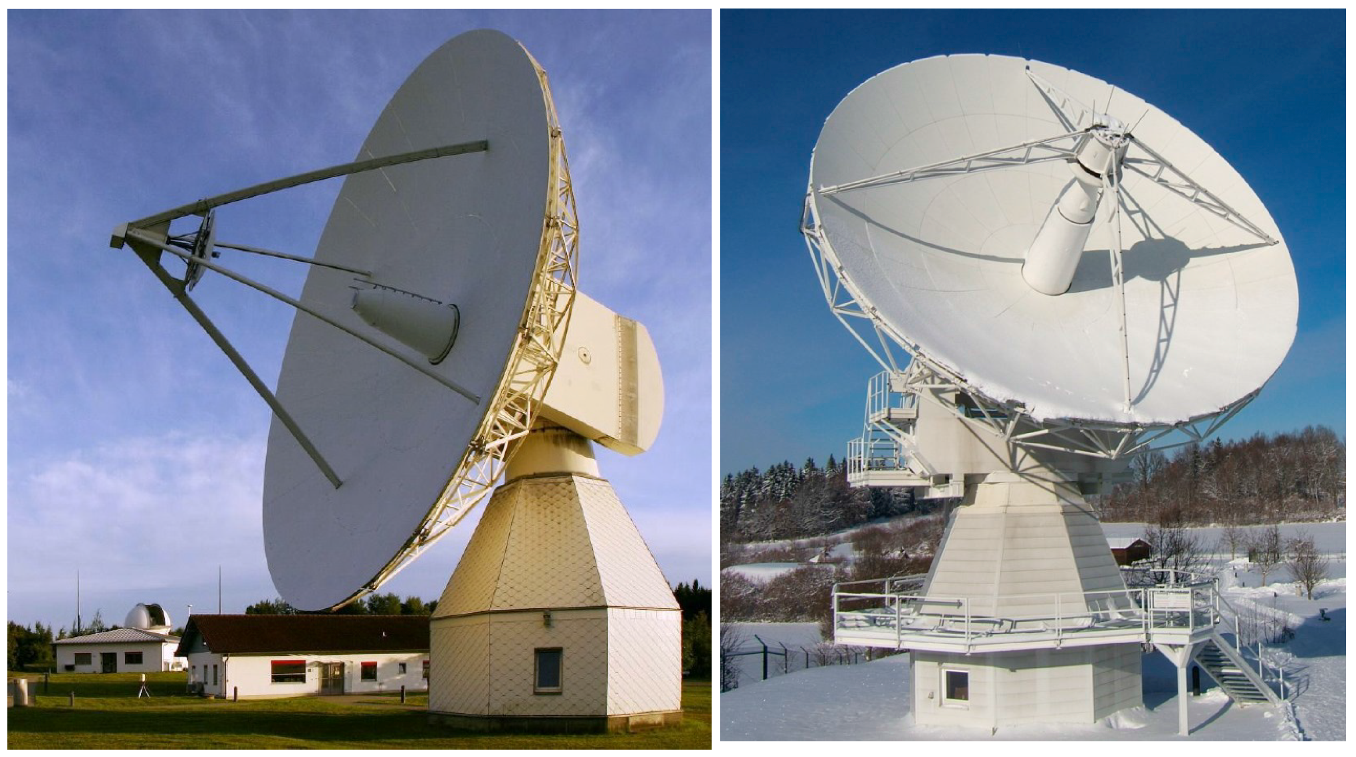
Funding

This research received no external funding.

Acknowledgments

The research was conducted in the framework of LEVIKA (Local VLBI Correlation and Analysis) project funded by the Federal Agency for Cartography and Geodesy (BKG). The author would like to especially thank colleagues (Walter Alef and Helge Rottmann) from MPIfR for providing the hardware and necessary input for the installation of computing cluster and correlation software at GOW. We would also like to show our gratitude to the fellow employees (Laura La Porta and Simone Bernhart) from Reichert GmbH/Bundesamt für Kartographie und Geodäsie for sharing their pearls of wisdom with us during the course of this research. The author would like to gratefully acknowledge the software correlator (DiFX) used for correlating the dataset presented in this paper. The software correlator was developed at the Swinburne University of Technology as part of the Australian Major National Research Facilities Programme and operated under license. We thank the reviewers for their comments and suggestions.

Conflicts of Interest

The authors declare no conflict of interest.

Abbreviations

The following abbreviations are used in this manuscript:
VLBIVery Long Baseline Interferometry
IVSInternational VLBI Service for Geodesy and Astronomy
DiFXDistributed Fourier transform (F) and a cross-multiplication (X)
HOPSHaystack Observatory Postprocessing System
ASCIIAmerican Standard Code for Information Interchange
VieVSVienna VLBI and Satellite Software
EOPEarth Orientation Parameter
NetCDFNetwork Common Data Form
GUIGraphical User interface
FSField System
UPSUninterruptible power supply
UT1Universal Time
GPSGlobal Positioning System
vgosDBVLBI Global Observation System Data Base
VGOSVLBI Global Observation System
UTCCoordinated Universal Time
GSFCGoddard Space Flight Center
SNRSignal to Noise Ratio
FTPFile Transfer Protocol
GbpsGigabytes per second
RHCPRight Hand Circular Polarization
LEVIKALocal VLBI Korrelation and Analysis
MPIfRMax-Planck-Institute for Radio astronomy
DBBCDigital Base-Band Converter
LOLocal Oscillator
BBCBase-Band Channel
IFIntermediate frequency
SEFDSystem Equivalent Flux Density
RFIRadio Frequency Interference

References

  1. Maehler, S.; Schade, C.; Kluegel, T. Local ties at the Geodetic Observatory Wettzell. In Proceedings of the EGU General Assembly 2010, Vienna, Austria, 2–7 May 2010; Volume 12, p. 4815. [Google Scholar]
  2. Neidhardt, A.; Kronschnabl, G.; Schatz, R. Geodetic Observatory Wettzell 20-m Radio Telescope and Twin Telescope. In International VLBI Service for Geodesy and Astrometry 2012 Annual Report; Behrend, D., Baver, K.D., Armstrong, K.L., Eds.; 2013; pp. 169–172. Available online: https://ivscc.gsfc.nasa.gov/publications/ar2012/IVS-2012-Annual-Report.pdf (accessed on 27 November 2018).
  3. International VLBI Service for Geodesy and Astrometry. Available online: https://ivscc.gsfc.nasa.gov/index.html (accessed on 27 November 2018).
  4. Schüler, T.; Plötz, C.; Phogat, A. BKG CVC—The Central VLBI Observation Coordination Facility of the Federal Agency for Cartography and Geodesy at the Geodetic Observatory Wettzell. In Proceedings of the IVS General Meeting, Svalbard, Norway, 3–8 June 2018. [Google Scholar]
  5. Schüler, T.; Kronschnabl, G.; Plötz, C.; Neidhardt, A.; Bertarini, A.; Bernhart, S.; Porta, L.l.; Halsig, S.; Nothnagel, A. Initial results obtained with the first TWIN VLBI radio telescope at the Geodetic Observatory Wettzell. Sensors 2015, 15, 18767–18800. [Google Scholar] [CrossRef] [PubMed]
  6. Kronschnabl, G.; Schüler, T.; Neidhardt, A.; Plötz, C.; Klügel, T.; Kodet, J. Status of the Wettzell Radio Telescope Triple and the O’Higgins VLBI System at Antarctica. In International VLBI Service for Geodesy and Astrometry 2014 General Meeting Proceedings: “VGOS: The New VLBI Network”; Behrend, D., Baver, K.D., Armstrong, K.L., Eds.; Science Press: Beijing, China, 2014; pp. 145–149. ISBN 978-7-03-042974-2. [Google Scholar]
  7. Deller, A.T.; Tingay, S.; Bailes, M.; West, C. DiFX: A software correlator for very long baseline interferometry using multiprocessor computing environments. Publ. Astron. Soc. Pac. 2007, 119, 318–336. [Google Scholar] [CrossRef]
  8. Deller, A.; Brisken, W.; Phillips, C.; Morgan, J.; Alef, W.; Cappallo, R.; Middelberg, E.; Romney, J.; Rottmann, H.; Tingay, S.; et al. DiFX-2: A more flexible, efficient, robust, and powerful software correlator. Publ. Astron. Soc. Pac. 2011, 123, 275–287. [Google Scholar] [CrossRef]
  9. Rogers, A.E.; Cappallo, R.J.; Hinteregger, H.F.; Levine, J.I.; Nesman, E.F.; Webber, J.C.; Whitney, A.R.; Clark, T.A.; Ma, C.; Ryan, J.; et al. Very-long-baseline radio interferometry: The Mark III system for geodesy, astrometry, and aperture synthesis. Science 1983, 219, 51–54. [Google Scholar] [CrossRef] [PubMed]
  10. Alef, W. Scheduling, Correlating, and Postprocessing of VLBI Observations. In Very Long Baseline Interferometry; Springer: Dordrecht, The Netherlands, 1989; pp. 97–139. [Google Scholar]
  11. Gipson, J. An introduction to Sked. In Proceedings of the Sixth General Meeting of the International VLBI Service for Geodesy and Astrometry, Tasmania, Australia, 7–14 February 2010; pp. 77–84. [Google Scholar]
  12. Gipson, J. Sked–VLBI Scheduling Software; NASA Goddard Space Flight Center: Greenbelt, MD, USA, 2012.
  13. Sun, J.; Böhm, J.; Nilsson, T.; Krásná, H.; Böhm, S.; Schuh, H. New VLBI2010 scheduling strategies and implications on the terrestrial reference frames. J. Geod. 2014, 88, 449–461. [Google Scholar] [CrossRef] [PubMed] [Green Version]
  14. Vandenberg, N. Drudg: Experiment Preparation Drudge Work; Space Geodesy Program, VLBI Software Manual; NASA/Goddard Space Flight Center: Greenbelt, MD, USA, 1997.
  15. Himwich, E. Introduction to the field system for non-users. In International VLBI Service for Geodesy and Astrometry 2000 General Meeting Proceedings; National Aeronautics and Space Administration (NASA): Washington, DC, USA, 2000; pp. 86–90. [Google Scholar]
  16. Bolotin, S.; Baver, K.; Gipson, J.; Gordon, D.; MacMillan, D. The VLBI Data Analysis Software nuSolve: Development Progress and Plans for the Future. In International VLBI Service for Geodesy and Astrometry 2014 General Meeting Proceedings: “VGOS: The New VLBI Network”; Behrend, D., Baver, K.D., Armstrong, K.L., Eds.; Science Press: Beijing, China, 2014; pp. 253–257. ISBN 978-7-03-042974-2. [Google Scholar]
  17. Böckmann, S.; Artz, T.; Nothnagel, A.; Tesmer, V. International VLBI Service for Geodesy and Astrometry: Earth orientation parameter combination methodology and quality of the combined products. J. Geophys. Res. Solid Earth 2010, 115, B044404. [Google Scholar] [CrossRef]
  18. Altamimi, Z.; Collilieux, X.; Métivier, L. ITRF2008: An improved solution of the international terrestrial reference frame. J. Geod. 2011, 85, 457–473. [Google Scholar] [CrossRef]
  19. Böhm, J.; Böhm, S.; Boisits, J.; Girdiuk, A.; Gruber, J.; Hellerschmied, A.; Krásná, H.; Landskron, D.; Madzak, M.; Mayer, D.; et al. Vienna VLBI and satellite software (VieVS) for geodesy and astrometry. Public. Astron. Soc. Pac. 2018, 130, 044503. [Google Scholar] [CrossRef]
  20. Vandenberg, N. Standard Schedule File Format, VLBI Software Documentation, Scheduling Program, Program Reference Manual, NASA/Goddard Flight Center, Space Geodesy Program. 1997. Available online: ftp://ftp.ga.gov.au/geodesy-outgoing/vlbi/dele405/Jupiter/2011/SKED.pdf (accessed on 3 December 2018).
  21. VEX File Definition/Example. Available online: https://vlbi.org/vex/docs/vex (accessed on 3 August 2018).
  22. Field System (FS) Documents. Available online: https://vlbi.gsfc.nasa.gov/fsdoc/ (accessed on 1 December 2018).
  23. Ambrosini, R.; Clark, T.; Corey, B.; Himwich, E. IVS Recommended Maser Timing Practices. 2014. Available online: https://ivscc.gsfc.nasa.gov/publications/memos/ivs-2014-001v01.pdf (accessed on 27 November 2018).
  24. Petrov, L. Instrumental errors of geodetic VLBI. In International VLBI Service for Geodesy and Astrometry 2000 General Meeting Proceedings; National Aeronautics and Space Administration (NASA): Washington, DC, USA, 2000; pp. 230–235. [Google Scholar]
  25. Treuhaft, R.; Lanyi, G. The effect of the dynamic wet troposphere on radio interferometric measurements. Radio Sci. 1987, 22, 251–265. [Google Scholar] [CrossRef]
  26. Krügel, M.; Thaller, D.; Tesmer, V.; Rothacher, M.; Angermann, D.; Schmid, R. Tropospheric parameters: Combination studies based on homogeneous VLBI and GPS data. J. Geod. 2007, 81, 515–527. [Google Scholar] [CrossRef]
  27. Haystack Observatory Postprocessing System. Available online: https://www.haystack.mit.edu/tech/vlbi/hops.html (accessed on 31 July 2018).
  28. Petrachenko, W.; Behrend, D.; Hase, H.; Ma, C.; Niell, A.; Schuh, H.; Whitney, A. The VLBI2010 global observing system (VGOS). In Proceedings of the EGU General Assembly EGU General Assembly 2013, Vienna, Austria, 7–12 April 2013. [Google Scholar]
  29. Petrachenko, B.; Behrend, D.; Gipson, J.; Hase, H.; Ma, C.; MacMillan, D.; Niell, A.; Nothnagel, A.; Zhang, X. VGOS Observing Plan. In Proceedings of the 8th IVS General Meeting, VGOS: “The New VLBI Network”; Science Press: Beijing, China, 2014; pp. 16–19. [Google Scholar]
  30. Gipson, J.; Böhm, J.; Bolotin, S.; Gordon, D.; Hobiger, T.; Jacobs, C.; Kurdobov, S.; Nothnagel, A.; Sovers, O.; Titov, O.; et al. Final Report of IVS Working Group 4 (WG4) on Data Structures. In International VLBI Service for Geodesy and Astrometry 2013 Annual Report; NASA/TP-2014-217522; NASA GSFC: Greenbelt, MD, USA, 2014; pp. 11–25. [Google Scholar]
  31. Bolotin, S.; Baver, K.; Gipson, J.; Gordon, D.; MacMillan, D. Implementation of the vgosDb Format at the GSFC VLBI Analysis Center. In Proceedings of the 23rd European VLBI Group for Geodesy and Astrometry Working Meeting, Göteborg, Sweden, 14–19 May 2017; pp. 235–237. [Google Scholar]
  32. Thorandt, V.; Wojdziak, R. BKG Data Center; NASA Goddard Space Flight Center: Greenbelt, MD, USA, 2008; p. 161.
  33. Abidin, Z.Z.; Ibrahim, Z.A.; Rosli, Z.; Malim, S.F.F.; Anim, N.M.; Noorazlan, N. An RFI investigation for setting up a VLBI station below 2.8 GHz in Malaysia. New Astron. 2012, 17, 61–64. [Google Scholar] [CrossRef]
  34. NGS Card File Format. Available online: https://vlbi.gsfc.nasa.gov/global/ngs-doc.html (accessed on 25 October 2018).
  35. Schüler, T.; Plötz, C.; Phogat, A. LEVIKA SBA—Wettzell Radio-Telescope Positioning with a Tailor-Made Analysis Software. In Proceedings of the IVS General Meeting, Svalbard/Norwegen, Norway, 3–8 June 2018. [Google Scholar]
Figure 1. Image of Radio Telescope Wettzell (RTW) on the left and one of the twin telescopes in Wettzell (TTW1) on the right.
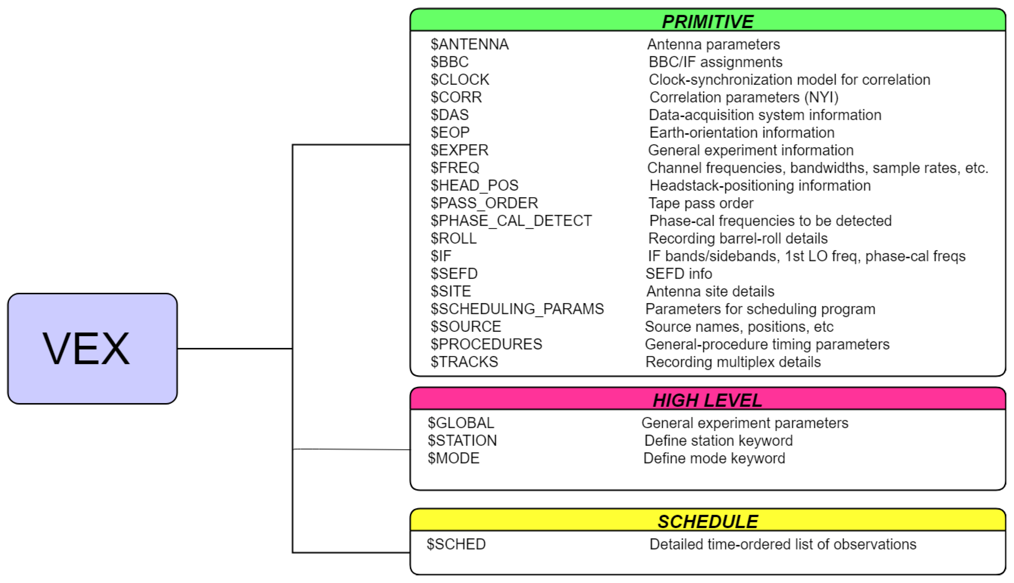
Data 03 00064 g001
Figure 2. Important blocks with the description in a .vex file.
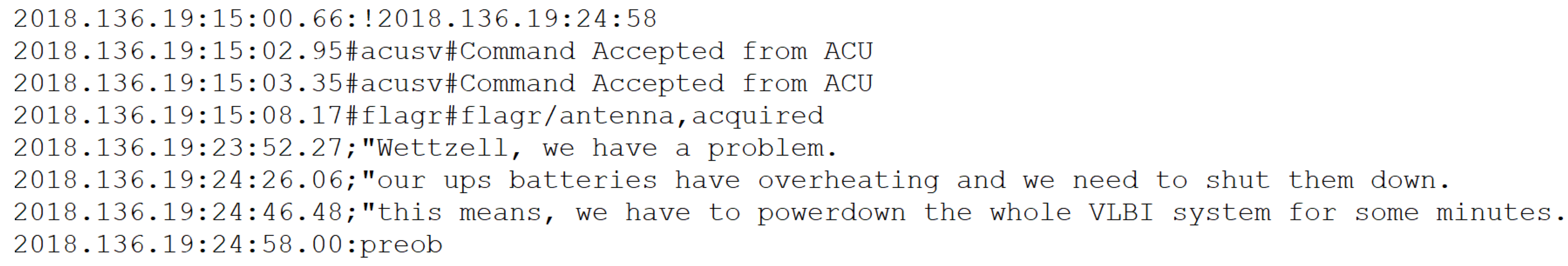
Data 03 00064 g002
Figure 3. Screen shot from a log file where the operator is informing about the overheated UPS during the observation. These comments help correlation and analysis center in understanding the reasons for missing scans.
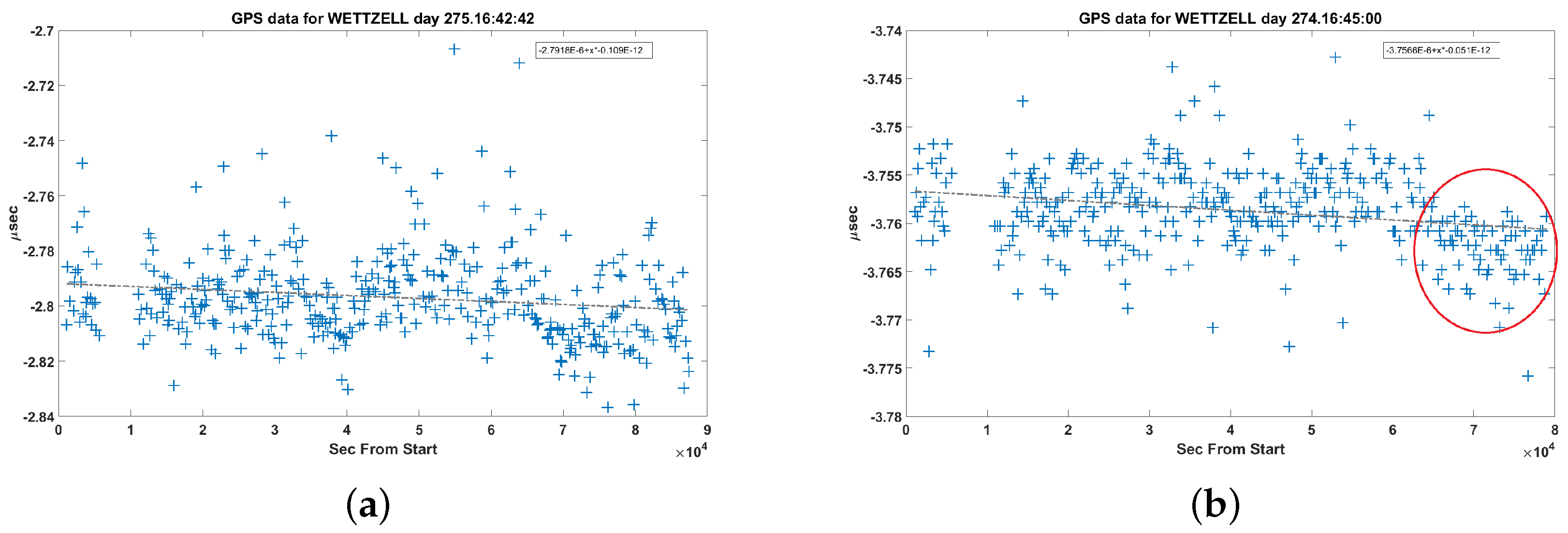
Data 03 00064 g003
Figure 4. Clock-offset vs. observation time extracted from the log file for WETTZELL station. Offset values for each observed scan are represented in blue. The trend line is in grey. (a) Plot from 18OCT15XA; (b) Plot from 18OCT01XA.
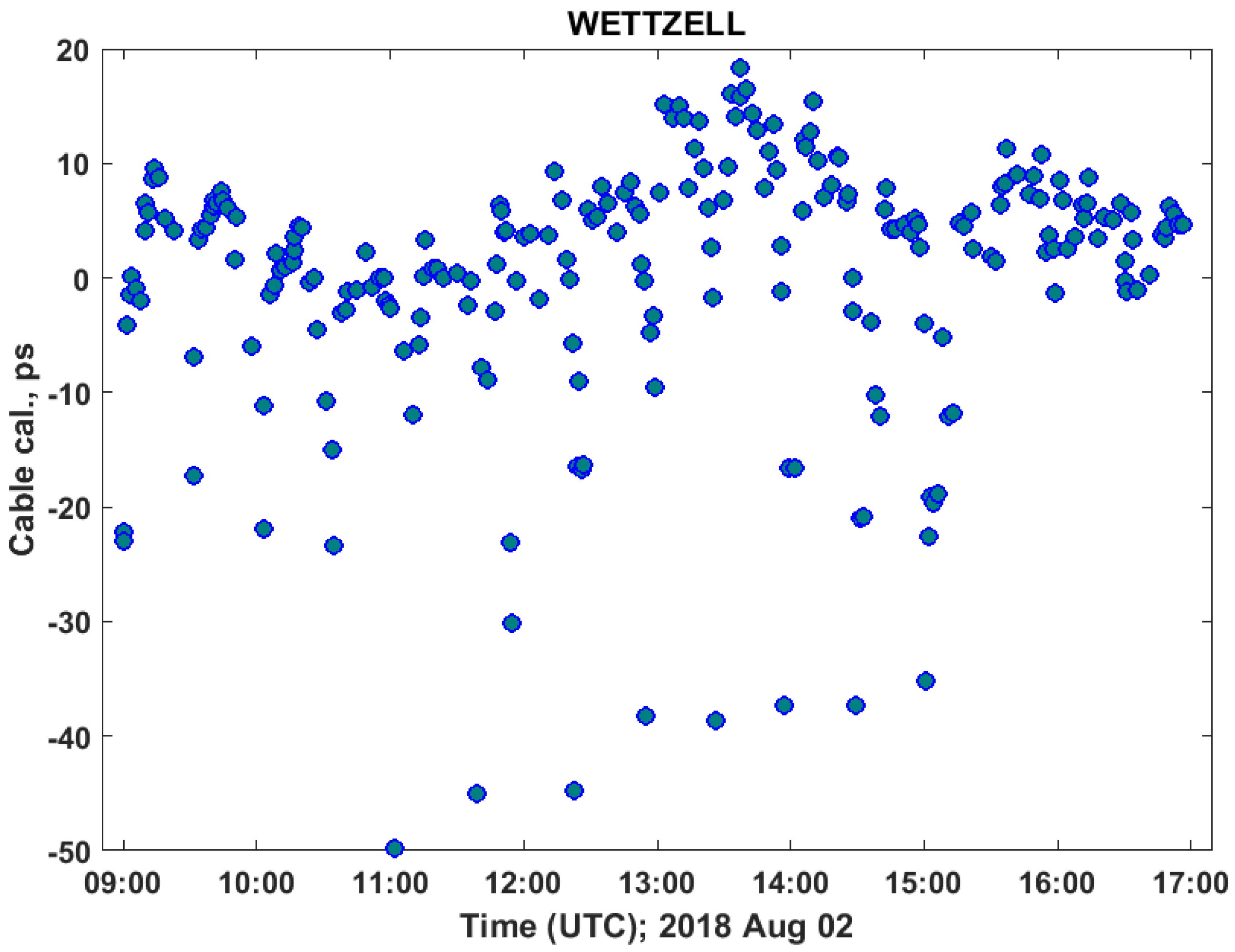
Data 03 00064 g004
Figure 5. Cable delay versus time from a local session 18AUG02X9 for WETTZELL station.
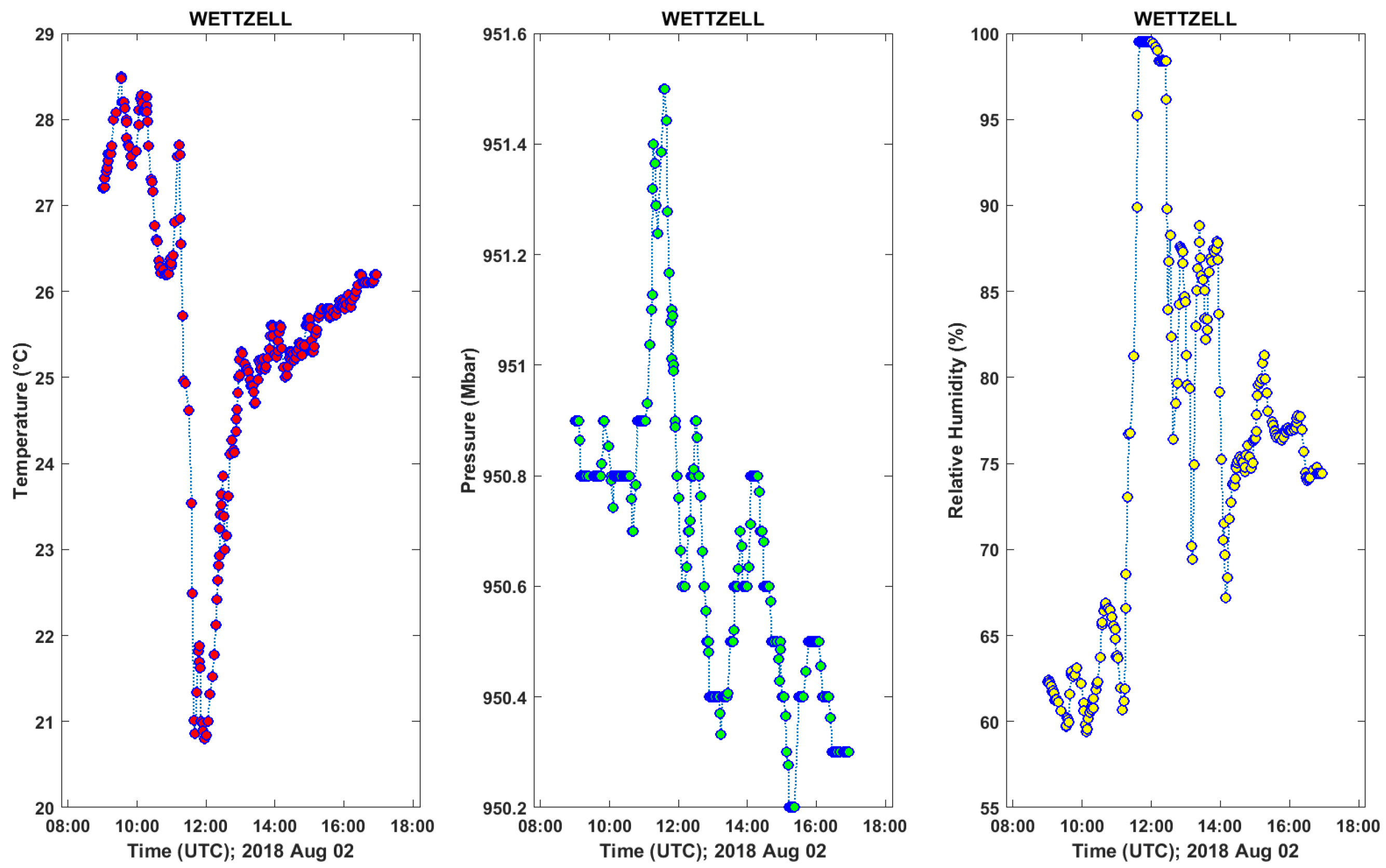
Data 03 00064 g005
Figure 6. Meteorological dataset extracted from the NetCDF file. The dataset from both the telescopes are collected from the same sensor, hence the values are exactly the same for the other telescope as well.
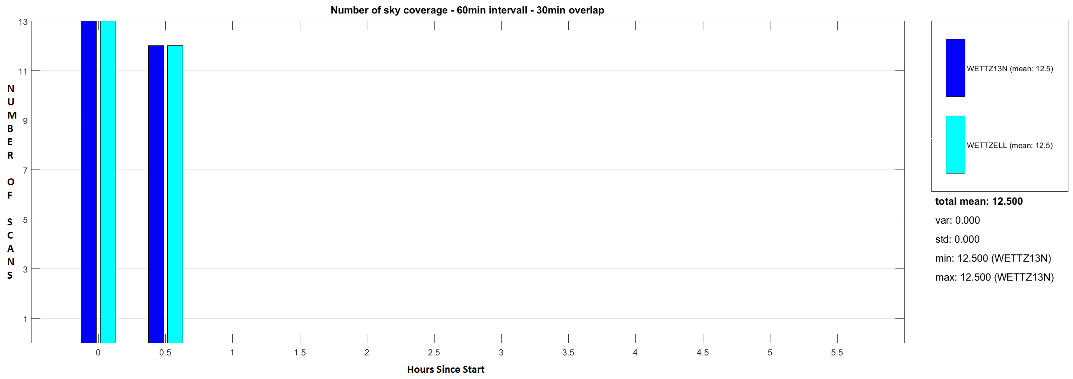
Data 03 00064 g006
Figure 7. Sky-coverage histogram plot vs observation time for all the participating telescopes.
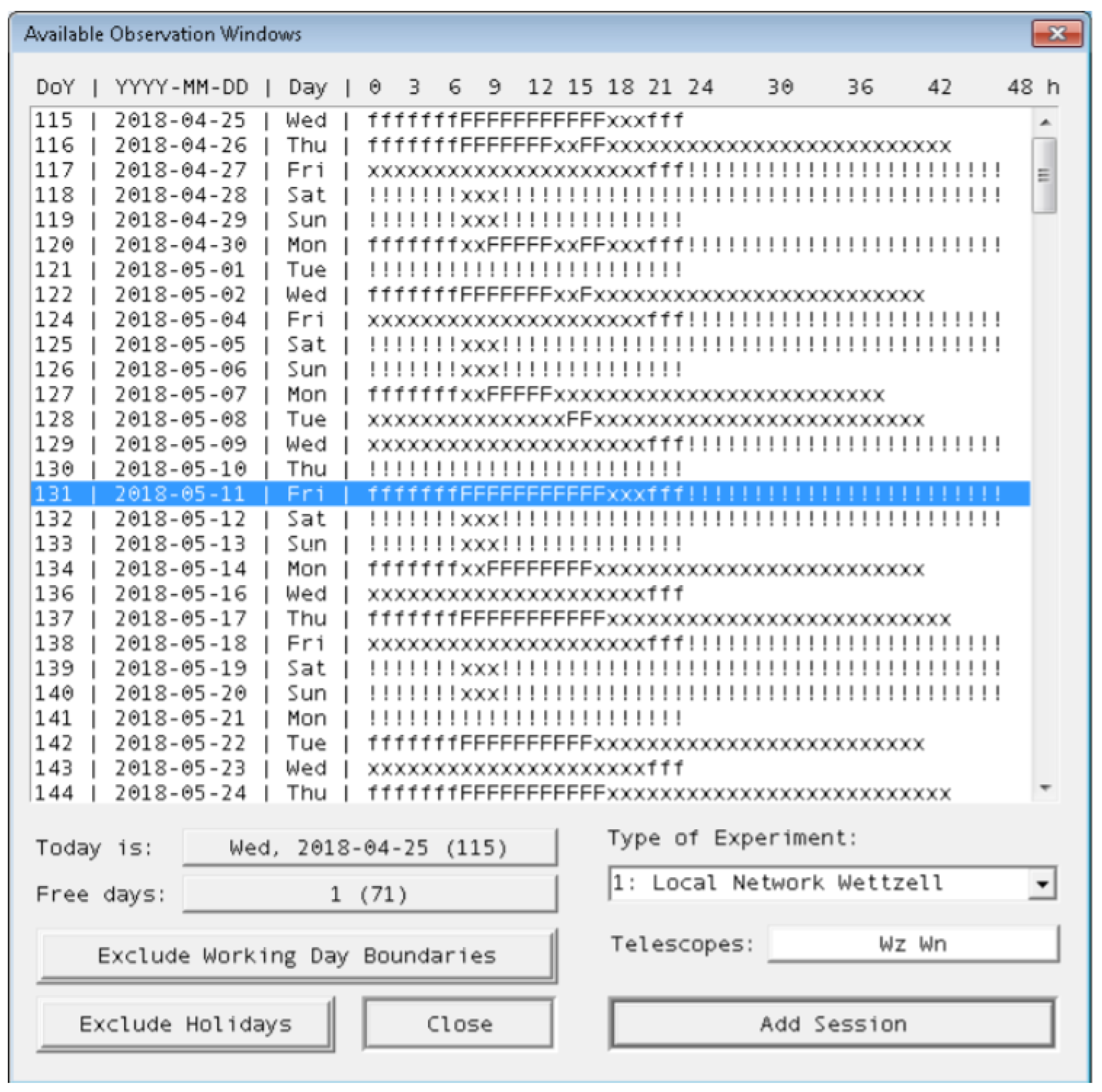
Data 03 00064 g007
Figure 8. Screen shot of the coordination tool with the available time slots for Wn-Wz baseline.
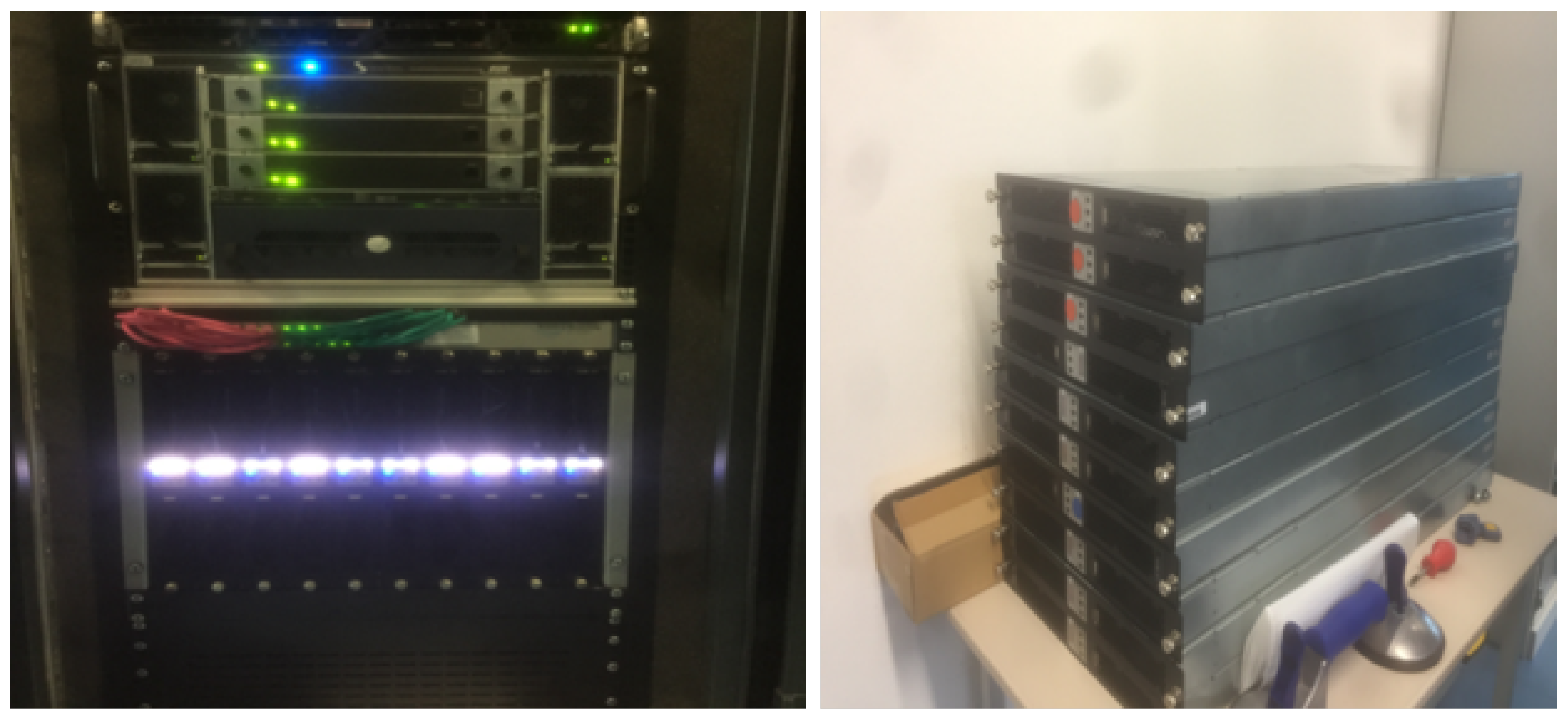
Data 03 00064 g008
Figure 9. Image of the computing cluster installed at the TWIN operations room with the spare nodes.
Data 03 00064 g009
Figure 10. Example of a fringe plot from a local session.
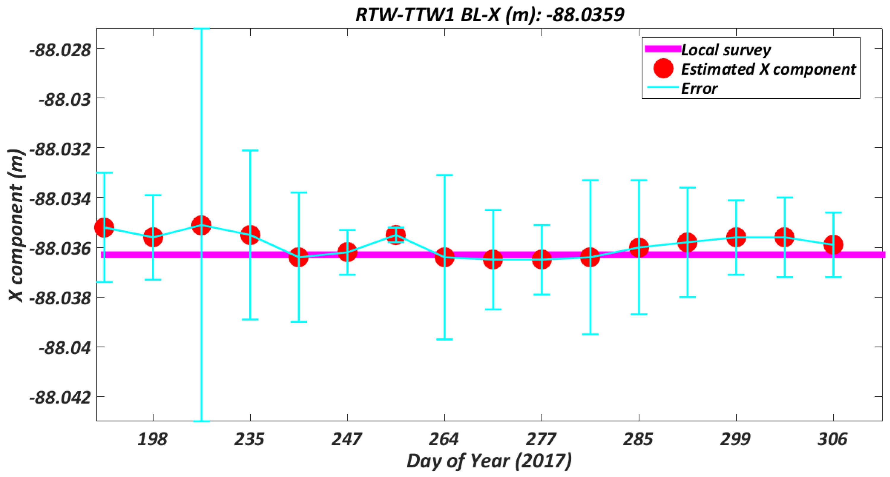
Data 03 00064 g010
Figure 11. Estimated X-component from short baseline observations in 2017.
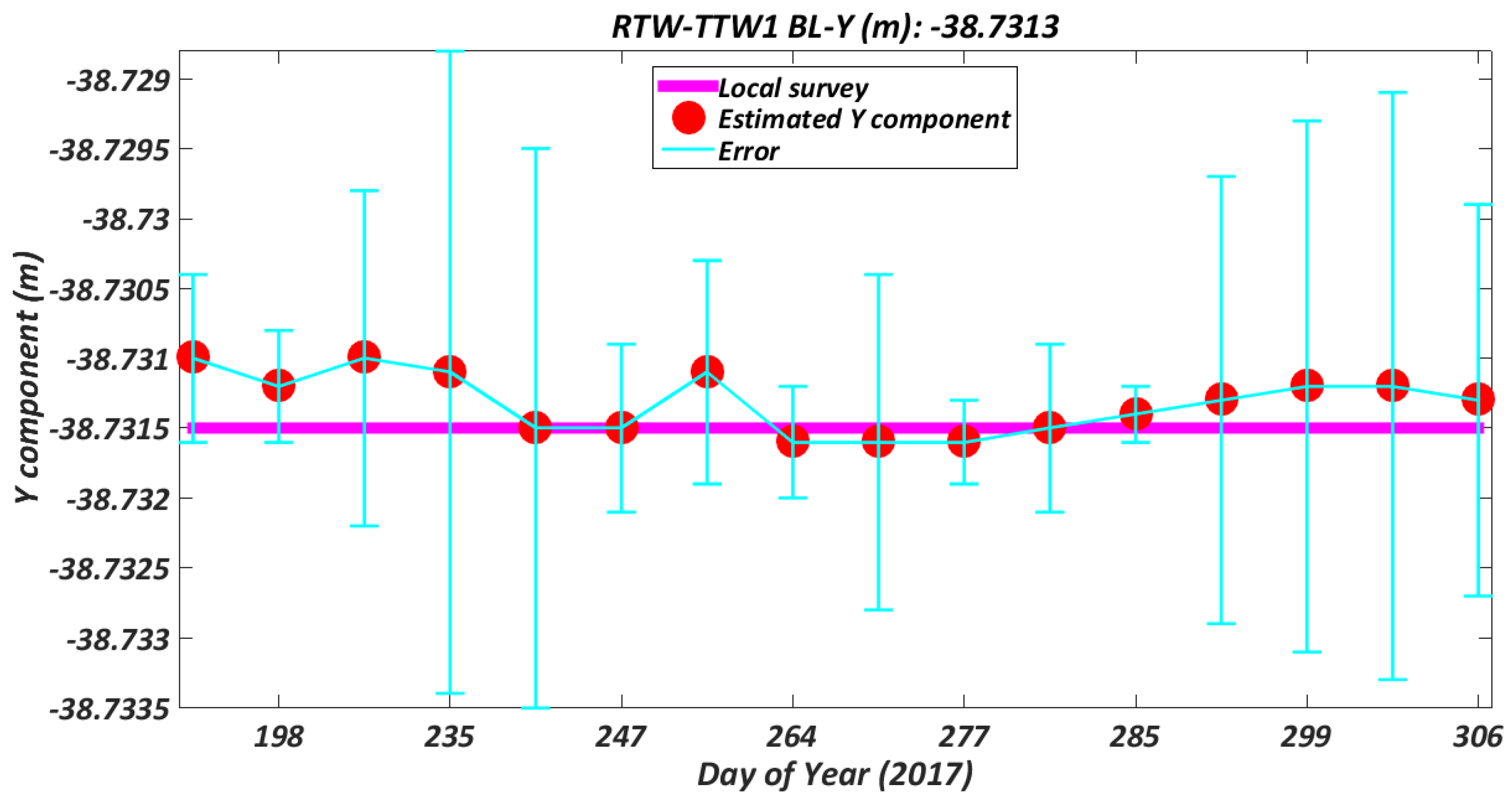
Data 03 00064 g011
Figure 12. Estimated Y-component from short baseline observations in 2017.
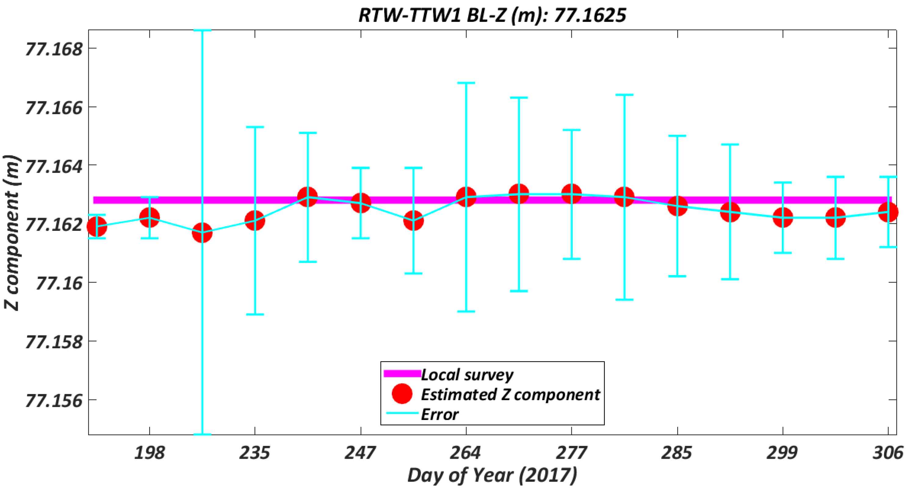
Data 03 00064 g012
Figure 13. Estimated Z-component from short baseline observations in 2017.
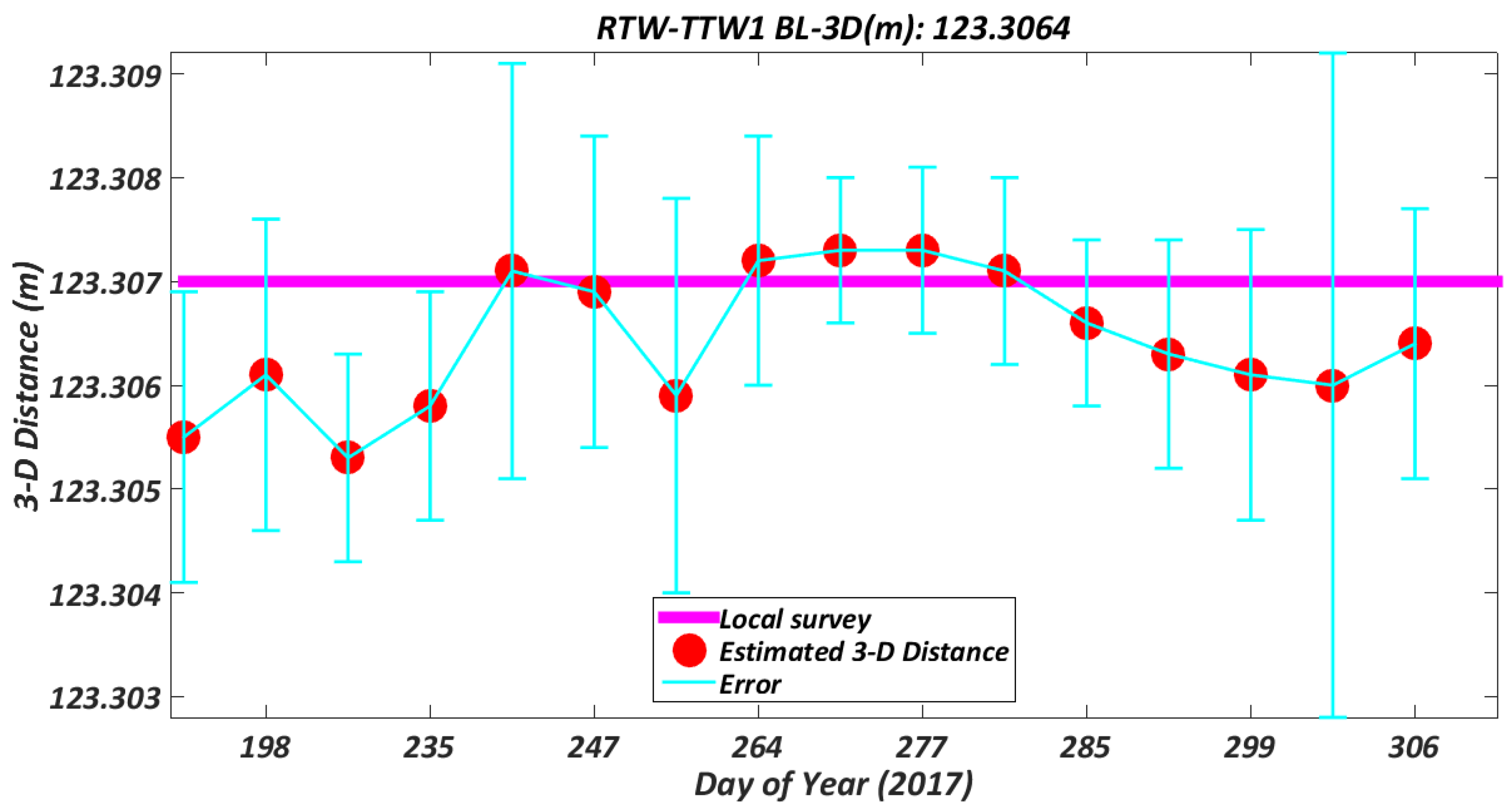
Data 03 00064 g013
Figure 14. Estimated 3-D distance from short baseline observations in 2017.
Data 03 00064 g014
Table 1. VLBI Session Distribution for 2017.
Session NameWzWnTotal
IVS-R1472673
IVS-R4492776
IVS-T27-7
EUROPE224
VLBA549
R& D14418
CONT151530
INT12284232
INT21012103
INT3404484
GOW303565
Total538163701
Table 2. Technical specifications of the participating telescopes.
AntennaDiameter (m)Front-endBack-end
Wz20Dual-band (S/X)DBBC
Wn13.2Tri-band (S/X/Ka)DBBC
Table 3. Important sections with the description in the .skd file.
SectionDescription
$EXPERExperiment title
$PARAMParameters used by sked and drudg
$SOURCESList of sources for this experiment
$STATIONSList of stations in this experiment
$FLUXFlux densities for each source
$CODESFrequency sequences and station LOs
$HEADTape recorder head position
$PROCStation procedures
$OPAutomatic scheduling options
$SKEDScheduled observations
Table 4. Important headers with the description in the alist.out file.
Header NameDescription
ROOTRoot code
F#Frequency subgroup
DURScan duration
EXP#Experiment number defined during difx2mark4
SCAN_IDScan identifier
YEARYear of observation
TIMETAGSTime in UTC
SOURCESource name
BSBaseline name given by 1 letter code
QFringe quality code
FM#CFrequency code with number of channels
PLPolarization
LAGSNumber of lags
SNRSignal to noise ratio
SBDLYSingle band delay
MBDLYMulti-band delay
DRATEDelay rate
ELEVATIONSource elevation angle
AZIMUTHSource azimuth angle
REF_FREQReference frequency defined in the control file during fringe fitting
TPHASETotal phase
TOTDRATETotal delay rate
TOTMBDELAYTotal multi-band delay
TOTSBDMMBDTotal single band delay minus multi-band delay
COHTIMESCoherence time
Table 5. List of files/folders in a VGOS database directory.
File / Folder NameDescription
Head.ncGeneral information about the session
sessionname_V001_kall.wrpWrapper file contains organisational information about the dataset
WETTZELL and WETTZ13NStation related information is stored in these folders
SolveInteger and fractional part of the time tag of scan
SessionInformation about fourfit output
ScanInformation about the observed scan and correlation root file
ObservablesInformation about observables of the session
ObsCalTheoInformation about theoretical observables
HistoryData processing history
Cross referencingCross referencing information between the observation and scan
Table 6. List of VLBI observables.
Observable NameDescription
AmbigSizeAmbiguity spacing size
BaselineSite names
Channel infoLocal oscillator and amplitude and phase information
CorrelationCorrelation coefficient
Corrinfo-difxFringe/fourfit related information
DataFlagDatabase flagging information
GroupDelayGroup delay
GroupRateDelay rate
PhaseTotal phase
PhaseCalInfoPhase calibration system details
QualityCodeFringe quality
RefFreqReference frequency defined in fringe fitting
SBDelaySingle band delay
SNRsignal to noise ratio
SOURCEList of sources
TimeUTCTime of observation in UTC
Table 7. NGS card file format.
Card NameDescription
Header cardGeneral information about the session
Site cardParticipating station information
Radio source positionObserved source position
Auxiliary parametersRef. frequency, group delay ambiguity spacing, delay type and rate information
Data cardsScan-wise information based on vex
Table 8. List of input files to the scheduling module.
File NameDescriptionType
Source.catSource location catalogueGSFC
Flux.catSource flux catalogueGSFC
Antenna.catSite catalogueGSFC
Position.catStation location catalogueGSFC
Equip.catHardware description catalogueGSFC
Mask.catElevation mask catalogueGSFC
Modes.catMeasurement mode catalogueGSFC
Freq.catFrequency setupGSFC
rx.catReceiving unitGSFC
loif.catLocal oscillator frequencyGSFC
rec.catData recording setupGSFC
hdpos.catHead position setupGSFC
tracks.catRecording tape setupGSFC
param.txtScheduling parameter definition fileLocal
down.txtDefine availability of stationLocal
snrmin.txtMinimum signal to noise ratioLocal
Psource.txtParticular source file mainly for astronomylocal
Table 9. Analysis results from sessions observed in 2017.
Baseline ComponentLocal Survey Measurement (m)VLBI Analysis (m)Offset (mm)
X−88.0363−88.03590.4
Y−38.7315−38.73130.2
Z77.162877.16250.3
3-D123.3070123.30640.6
Table 10. List of files provided in the dataset.
File/ Folder NameDescriptionFile Format
sessionname.skdSchedule fileASCII
sessionnamesiteid.logStation logASCII
sessionname.vexVLBI experiment fileASCII
alist.outfringe fitting outputASCII
vgosDBVGOS databaseASCII and NetCDF
NGS Filegroup delay informationASCII

