
Virtual Joint Motion Simulator Accurately Predicts Effects of Femoral Component Malalignment during TKA
Abstract
:1. Introduction
2. Materials and Methods
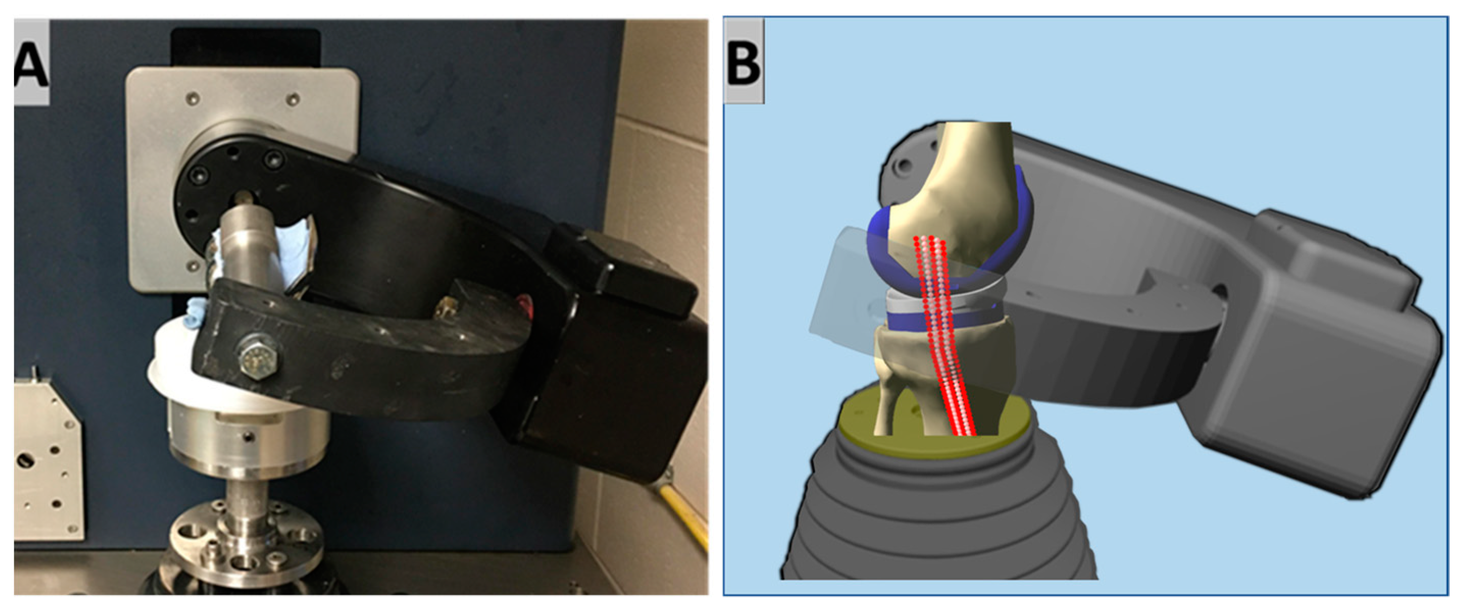
2.1. Virtual Simulator
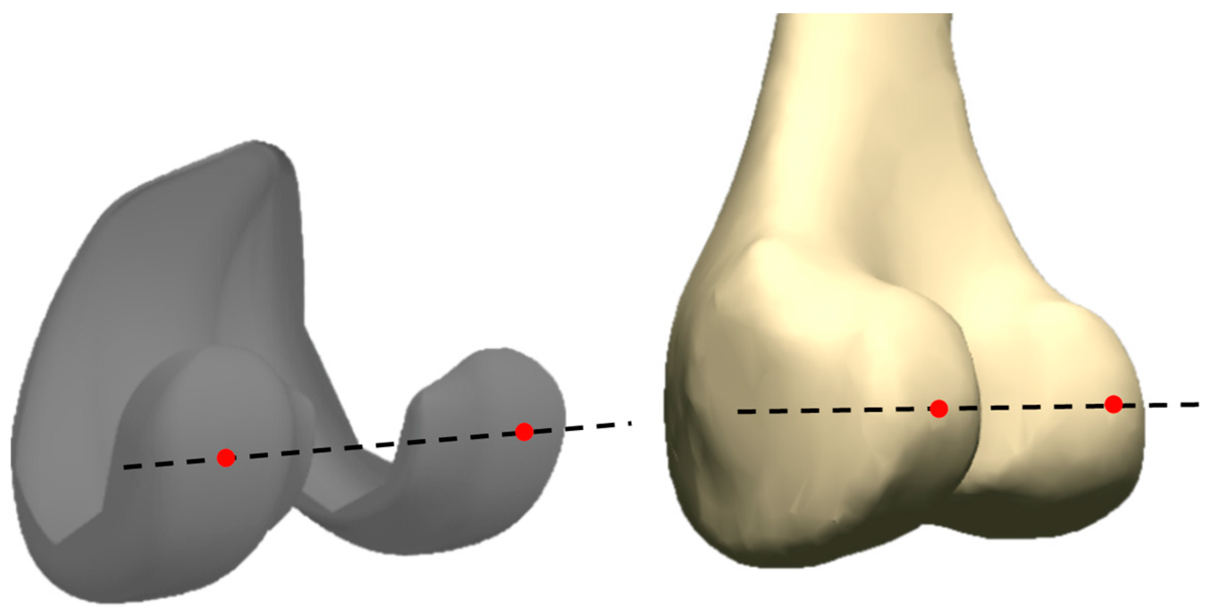
2.2. Knee Model
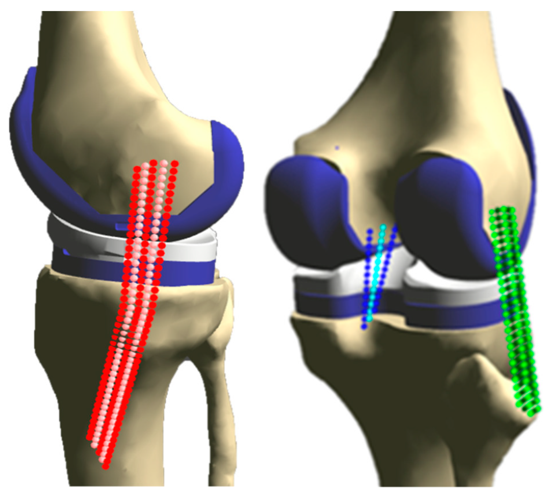
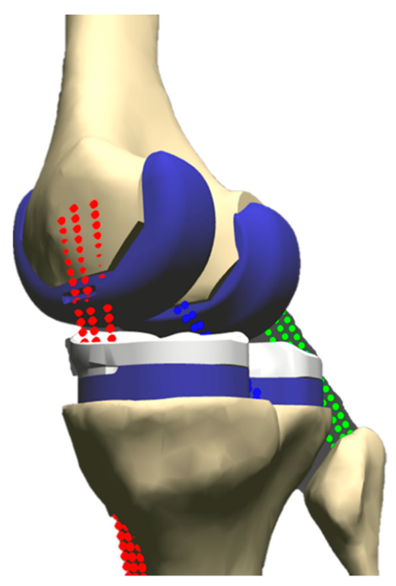
2.3. Ligament Model
2.4. Loading
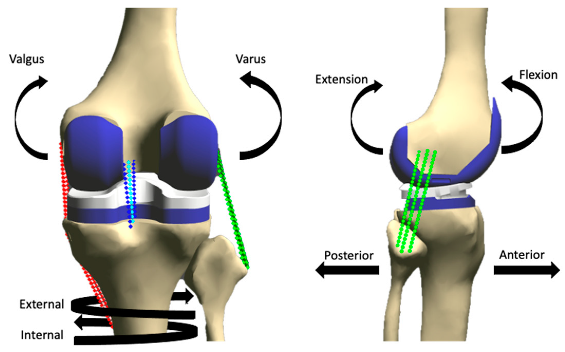
2.5. Data Analysis
3. Results
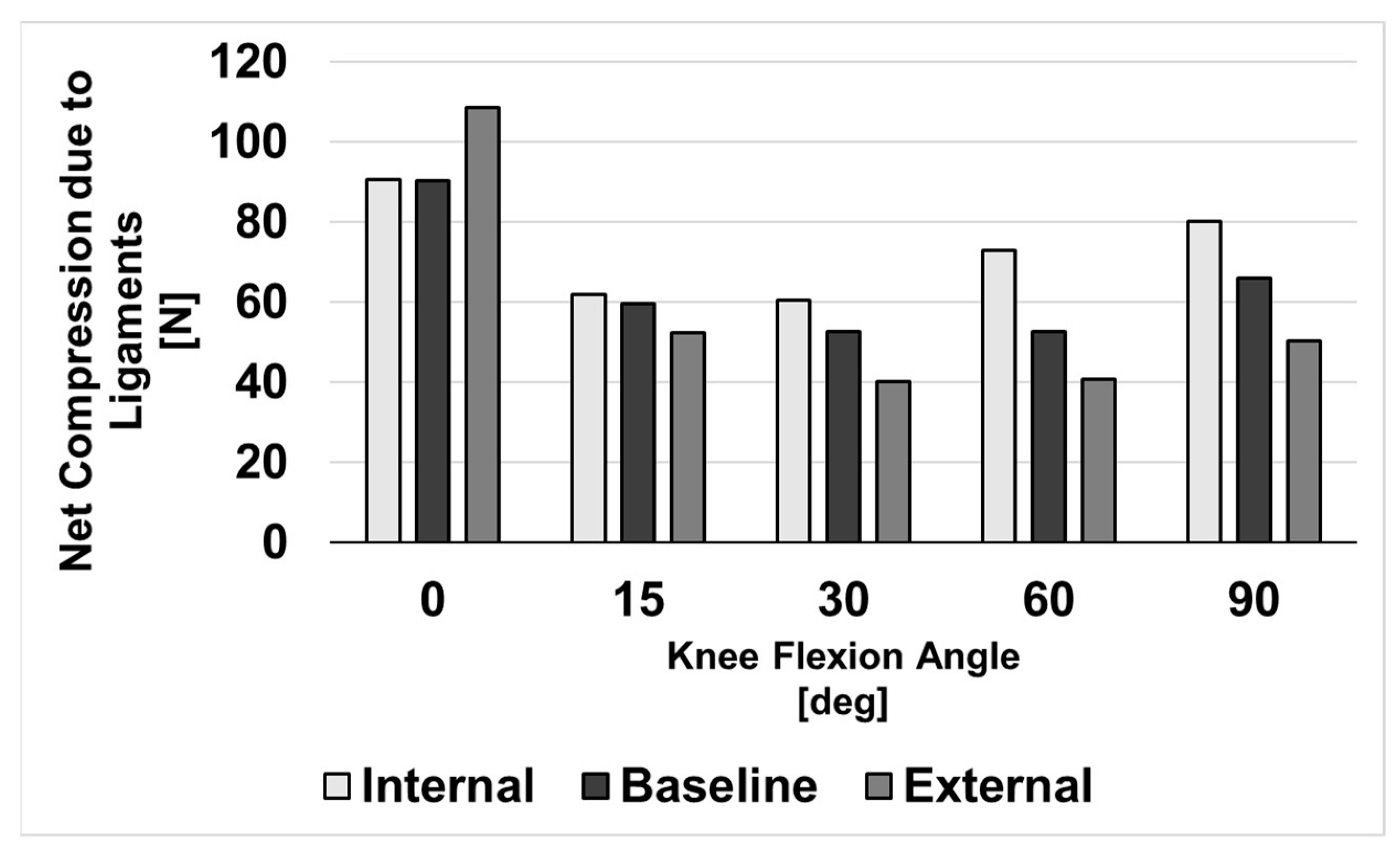
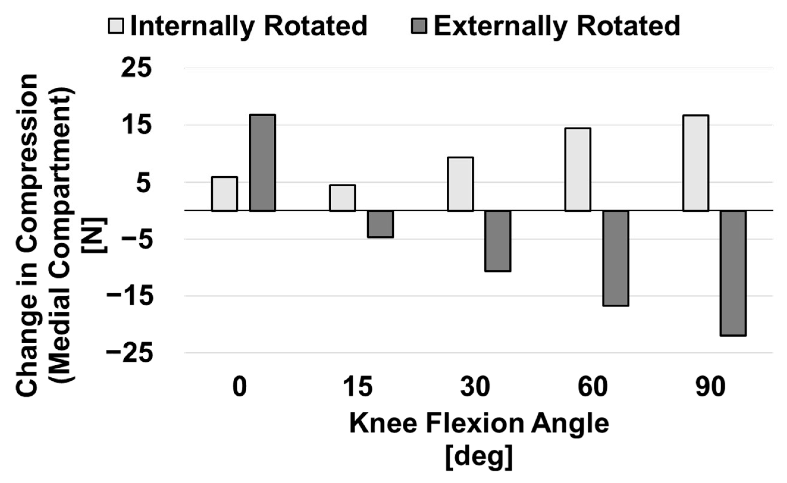
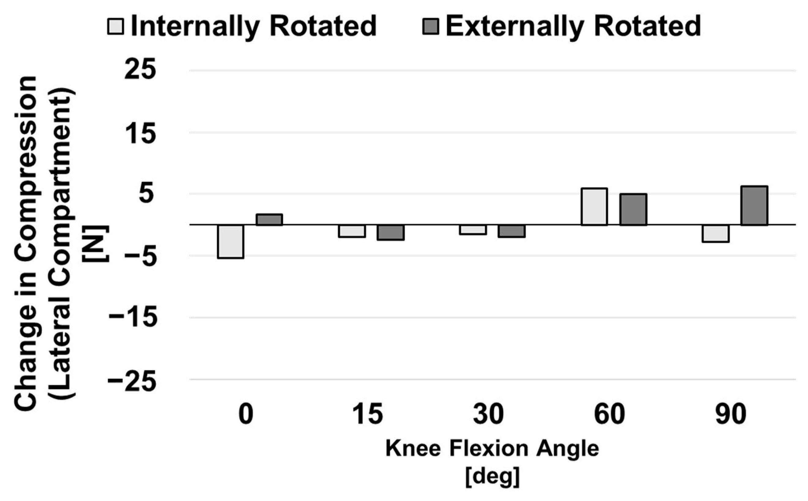
3.1. Compressive Ligament Forces during Neutral Flexion
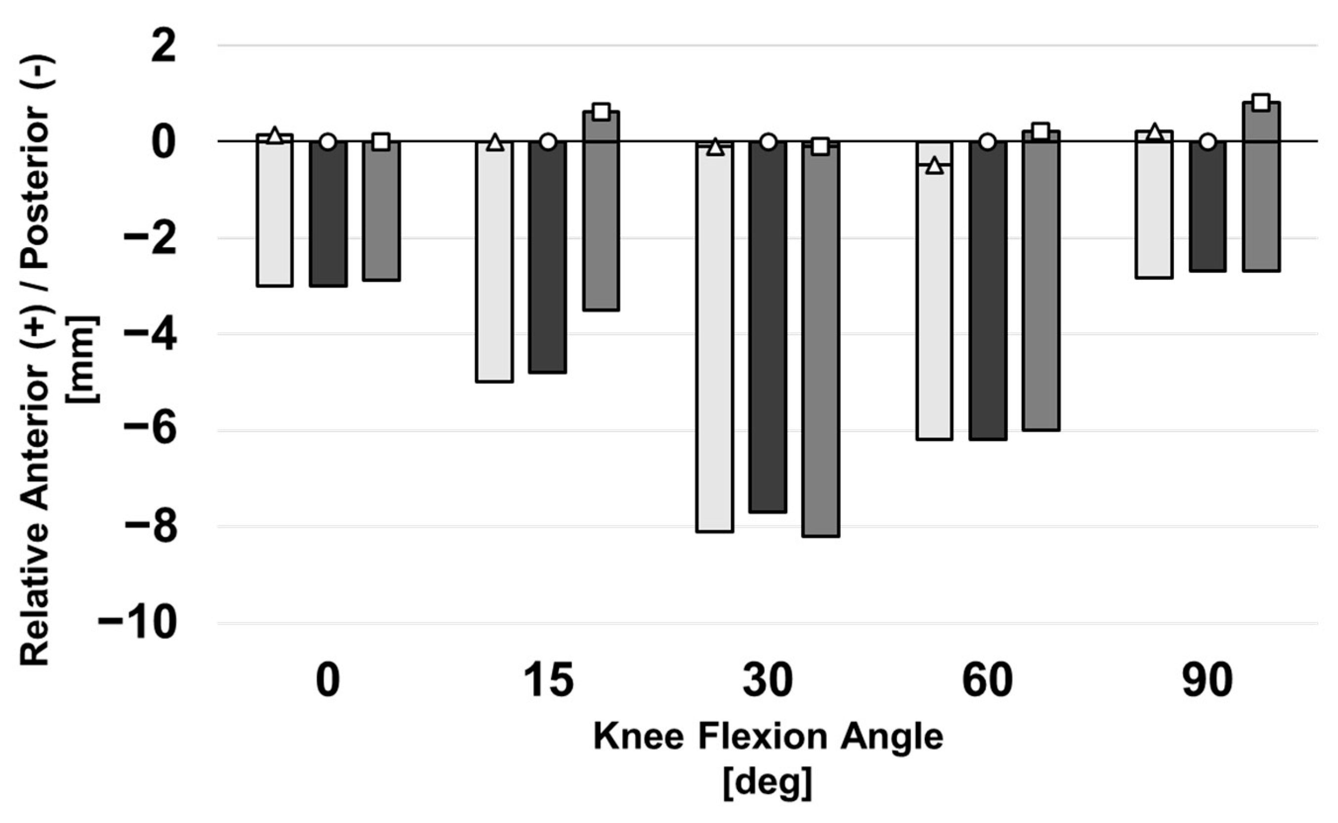
3.2. Posterior Laxity
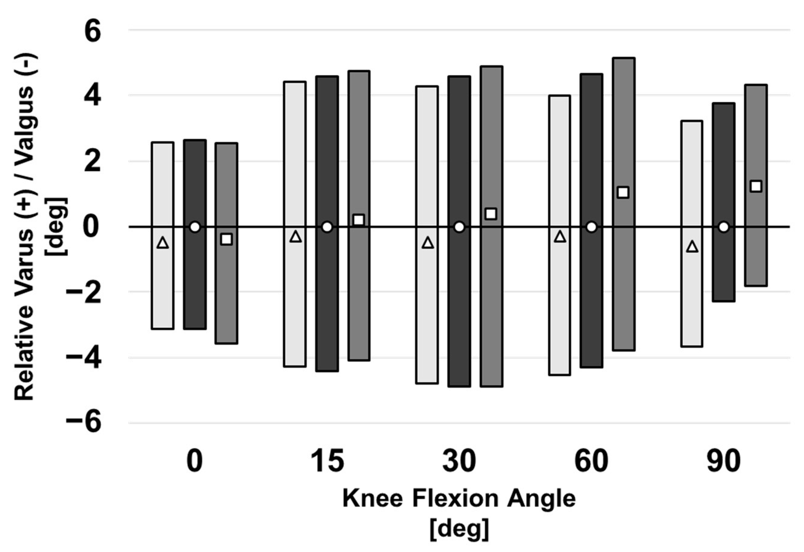
3.3. Varus–Valgus Laxity
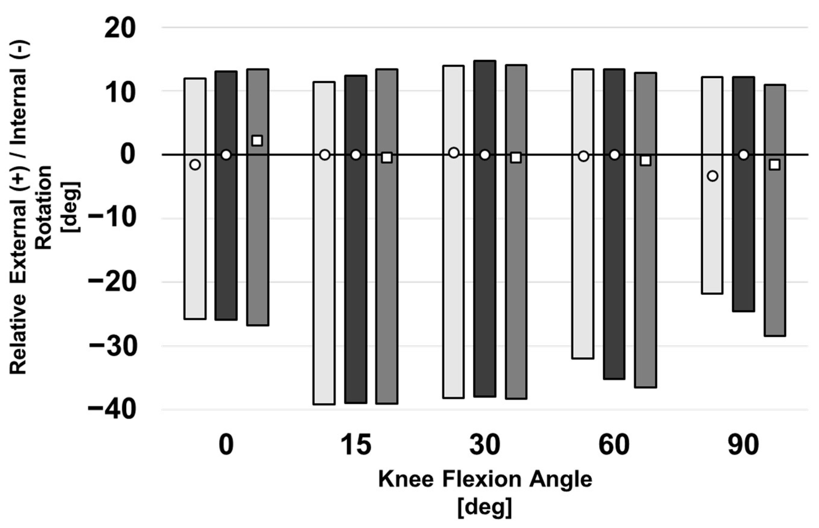
3.4. Internal–External Laxity
4. Discussion
5. Conclusions
Author Contributions
Funding
Institutional Review Board Statement
Data Availability Statement
Conflicts of Interest
Appendix A

References
- Inacio, M.C.S.; Paxton, E.W.; Graves, S.E.; Namba, R.S.; Nemes, S. Projected increase in total knee arthroplasty in the United States–An alternative projection model. Osteoarthr. Cartil. 2017, 25, 1797–1803. [Google Scholar] [CrossRef]
- Lau, R.L.; Gandhi, R.; Mahomed, S.; Mahomed, N. Patient Satisfaction after Total Knee and Hip Arthroplasty. Clin. Geriatric Med. 2012, 28, 349–365. [Google Scholar] [CrossRef]
- Bourne, R.B.; Chesworth, B.; Davis, A.; Mahomed, N.; Charron, K. Comparing patient outcomes after THA and TKA: Is there a difference? Clin. Orthop. Relat. Res. 2010, 468, 542–546. [Google Scholar] [CrossRef] [PubMed]
- Mahomed, N.; Gandhi, R.; Daltroy, L.; Katz, J.N. The Self-Administered Patient Satisfaction Scale for Primary Hip and Knee Arthroplasty. Arthritis 2011, 2011, 591253. [Google Scholar] [CrossRef] [PubMed]
- Abdelnasser, M.K.; Elsherif, M.E.; Bakr, H.; Mahran, M.; Othman, M.H.M.; Khalifa, Y. All types of component malrotation affect the early patient-reported outcome measures after total knee arthroplasty. Knee Surg. Relat. Res. 2019, 31, 5. [Google Scholar] [CrossRef]
- Naili, J.E.; Wretenberg, P.; Lindgren, V.; Iversen, M.D.; Hedström, M.; Broström, E.W. Improved knee biomechanics among patients reporting a good outcome in knee-related quality of life one year after total knee arthroplasty. BMC Musculoskelet Disord. 2017, 18, 122. [Google Scholar] [CrossRef]
- Hosseini, A.; Qi, W.; Tsai, T.Y.; Liu, Y.; Rubash, H.; Li, G. In vivo length change patterns of the medial and lateral collateral ligaments along the flexion path of the knee. Knee Surg. Sports Traumatol. Arthrosc. 2015, 23, 3055–3061. [Google Scholar] [CrossRef]
- Nasab, S.H.H.; List, R.; Oberhofer, K.; Fucentese, S.F.; Snedeker, J.G.; Taylor, W.R. Loading patterns of the posterior cruciate ligament in the healthy knee: A systematic review. PLoS ONE 2016, 11, e0167106. [Google Scholar]
- Boya, H.; Özcan, Ö.; Maralcan, G. An investigation of consistency between posterior condylar axis +3 degree external rotation line and clinical transepicondylar axis line techniques in primary total knee arthroplasty. Eklem Hastalik. Ve Cerrahisi 2014, 25, 70–74. [Google Scholar] [CrossRef]
- Lee, D.K.; Grosso, M.; Trofa, D.; Sonnefeld, J.; Cooper, H.; Shah, R.; Geller, J. Incidence of Femoral Component Malrotation Using Posterior Condylar Referencing in Total Knee Arthroplasty. J. Knee Surg. 2020, 33, 971–977. [Google Scholar] [CrossRef] [PubMed]
- Siston, R.A.; Patel, J.J.; Goodman, S.B.; Delp, S.L.; Giori, N.J. The Variability of Femoral Rotational Alignment in Total Knee Arthroplasty. J. Bone Joint Surg. 2005, 87, 2276–2280. [Google Scholar]
- Sternheim, A.; Lochab, J.; Drexler, M.; Kuzyk, P.; Safir, O.; Gross, A.; Backstein, D. The benefit of revision knee arthroplasty for component malrotation after primary total knee replacement. Int. Orthop. 2012, 36, 2473–2478. [Google Scholar] [CrossRef]
- Deck, J.; White, B. Joint-Relative Forces Using the Grood-Suntay Unit Vector Directions. Orthop. Proc. 2018, 98, 112. [Google Scholar]
- Willing, R.; Walker, P.S. Measuring the sensitivity of total knee replacement kinematics and laxity to soft tissue imbalances. J. Biomech. 2018, 77, 62–68. [Google Scholar] [CrossRef]
- Willing, R.; Moslemian, A.; Yamomo, G.; Wood, T.; Howard, J.; Lanting, B. Condylar-Stabilized TKR May Not Fully Compensate for PCL-Deficiency: An In Vitro Cadaver Study. J. Orthopaedic. Res. 2019, 37, 2172–2181. [Google Scholar] [CrossRef] [PubMed]
- Sekeitto, A.R.; McGale, J.G.; Montgomery, L.A.; Vasarhelyi, E.M.; Willing, R.; Lanting, B.A. Posterior-stabilized total knee arthroplasty kinematics and joint laxity: A hybrid biomechanical study. Arthroplasty 2022, 4, 53. [Google Scholar] [CrossRef]
- Bloemker, K.H.; Guess, T.M.; Maletsky, L.; Dodd, K. Computational Knee Ligament Modeling Using Experimentally Determined Zero-Load Lengths. Open Biomed. Eng. J. 2012, 6, 33–41. [Google Scholar] [CrossRef] [PubMed]
- Guess, T.M.; Razu, S.; Jahandar, H. Evaluation of Knee Ligament Mechanics Using Computational Models. J. Knee Surg. 2016, 29, 126–137. [Google Scholar]
- TGuess, M.; Razu, S. Loading of the medial meniscus in the ACL deficient knee: A multibody computational study. Med. Eng. Phys. 2017, 41, 26–34. [Google Scholar]
- Tetreault, D.M.; Kennedy, F.E. Friction and Wear Behavior of Ultrahigh Molecular Weight Polyethylene on Co-C2 and Titanium Alloys in Dry and Lubricated. Wear 1989, 133, 295–307. [Google Scholar] [CrossRef]
- Halloran, J.P.; Petrella, A.J.; Rullkoetter, P.J. Explicit finite element modeling of total knee replacement mechanics. J. Biomech. 2005, 38, 323–331. [Google Scholar] [CrossRef]
- Lee, J.K.; Lee, S.; Chun, S.H.; Kim, K.T.; Lee, M.C. Rotational alignment of femoral component with different methods in total knee arthroplasty: A randomized, controlled trial. BMC Musculoskelet. Disord. 2017, 18, 217. [Google Scholar] [CrossRef] [PubMed]
- Crottet, D.; Kowal, J.; Sarfert, S.A.; Maeder, T.; Bleuler, H.; Nolte, L.P.; Dürselen, L. Ligament balancing in TKA: Evaluation of a force-sensing device and the influence of patellar eversion and ligament release. J. Biomech. 2007, 40, 1709–1715. [Google Scholar] [CrossRef]
- Seo, J.-G.; Moon, Y.-W.; Jo, B.-C.; Kim, Y.-T.; Park, S.-H. Soft Tissue Balancing of Varus Arthritic Knee in Minimally Invasive Surgery Total Knee Arthroplasty: Comparison between Posterior Oblique Ligament Release and Superficial MCL Release. Knee Surg. Relat. Res. 2013, 25, 60–64. [Google Scholar] [CrossRef]
- Jeffcote, B.; Nicholls, R.; Schirm, A.; Kuster, M.S. The Variation in Medial and Lateral Collateral Ligament Strain and Tibiofemoral Forces Following Changes in the Flexion and Extension Gaps in Total Knee Replacement a Laboratory Experiment Using Cadaver Knees. J. Bone Joint Surg. 2007, 89, 1528–1533. [Google Scholar] [CrossRef] [PubMed]
- Gromov, K.; Korchi, M.; Thomsen, M.G.; Husted, H.; Troelsen, A. What is the optimal alignment of the tibial and femoral components in knee arthroplasty? Acta. Orthop. 2014, 85, 480–487. [Google Scholar] [CrossRef] [PubMed]
- Montgomery, L.; Vakili, S.; Lanting, B.; Willing, R. Force Characterization of Soft Tissues in the Post-TKR Knee During Activities of Daily Living. Prog. Can. Mech. Eng. 2021, 4. [Google Scholar] [CrossRef]


| Ligament 1 | Stiffness (N/ɛ) | Reference Strain (%) |
|---|---|---|
| aLCL | 1157 | −2.66 |
| amLCL | 1171 | 0.68 |
| mLCL | 1175 | 4.02 |
| mpLCL | 1172 | 2.66 |
| pLCL | 1182 | 1.29 |
| a-sMCL | 1469 | −4.30 |
| am-sMCL | 1603 | 0.10 |
| m-sMCL | 1481 | 4.50 |
| mp-sMCL | 1509 | 4.47 |
| p-sMCL | 1105 | 4.44 |
| aPCL | 7841 | −28.6 |
| pPCL | 1026 | −26.3 |
Disclaimer/Publisher’s Note: The statements, opinions and data contained in all publications are solely those of the individual author(s) and contributor(s) and not of MDPI and/or the editor(s). MDPI and/or the editor(s) disclaim responsibility for any injury to people or property resulting from any ideas, methods, instructions or products referred to in the content. |
© 2023 by the authors. Licensee MDPI, Basel, Switzerland. This article is an open access article distributed under the terms and conditions of the Creative Commons Attribution (CC BY) license (https://creativecommons.org/licenses/by/4.0/).
Share and Cite
Montgomery, L.; Willing, R.; Lanting, B. Virtual Joint Motion Simulator Accurately Predicts Effects of Femoral Component Malalignment during TKA. Bioengineering 2023, 10, 503. https://doi.org/10.3390/bioengineering10050503
Montgomery L, Willing R, Lanting B. Virtual Joint Motion Simulator Accurately Predicts Effects of Femoral Component Malalignment during TKA. Bioengineering. 2023; 10(5):503. https://doi.org/10.3390/bioengineering10050503
Chicago/Turabian StyleMontgomery, Liam, Ryan Willing, and Brent Lanting. 2023. "Virtual Joint Motion Simulator Accurately Predicts Effects of Femoral Component Malalignment during TKA" Bioengineering 10, no. 5: 503. https://doi.org/10.3390/bioengineering10050503