
Machine Learning-Based Respiration Rate and Blood Oxygen Saturation Estimation Using Photoplethysmogram Signals
 , ,
, ,  ,
,  , , and
Abstract
: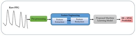
1. Introduction
- A unified ML system is proposed to estimate RR and SpO2 from PPG.
- Separate ML models are trained as RR, and SpO2 gives importance to different features.
- Analysis of the most important features to showcase which features predict RR or SpO2 the best.
2. Materials and Methods
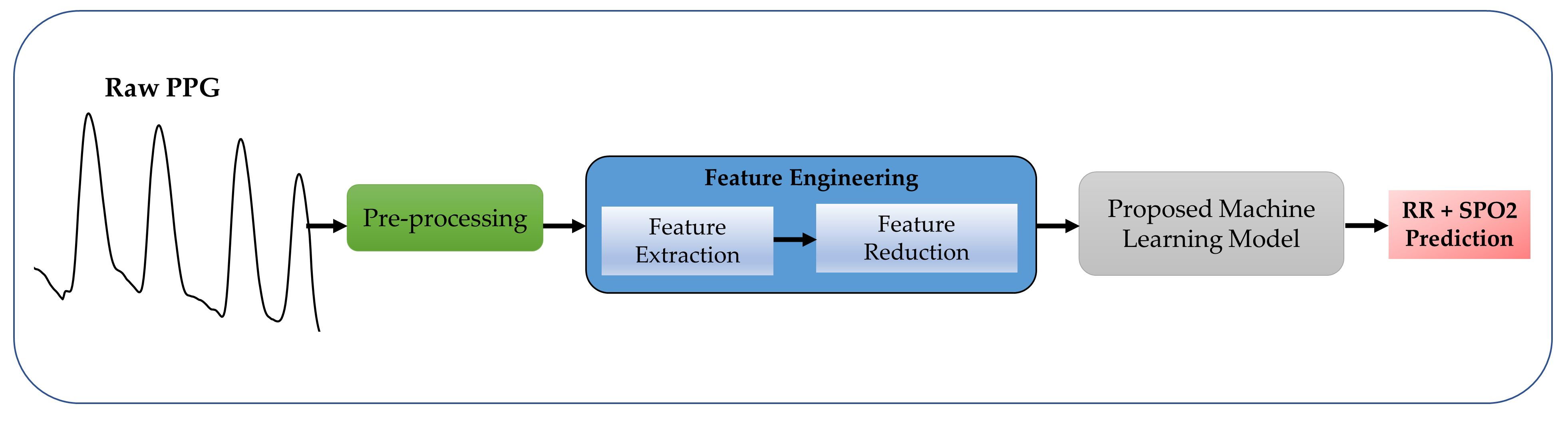
2.1. Dataset Descriptor
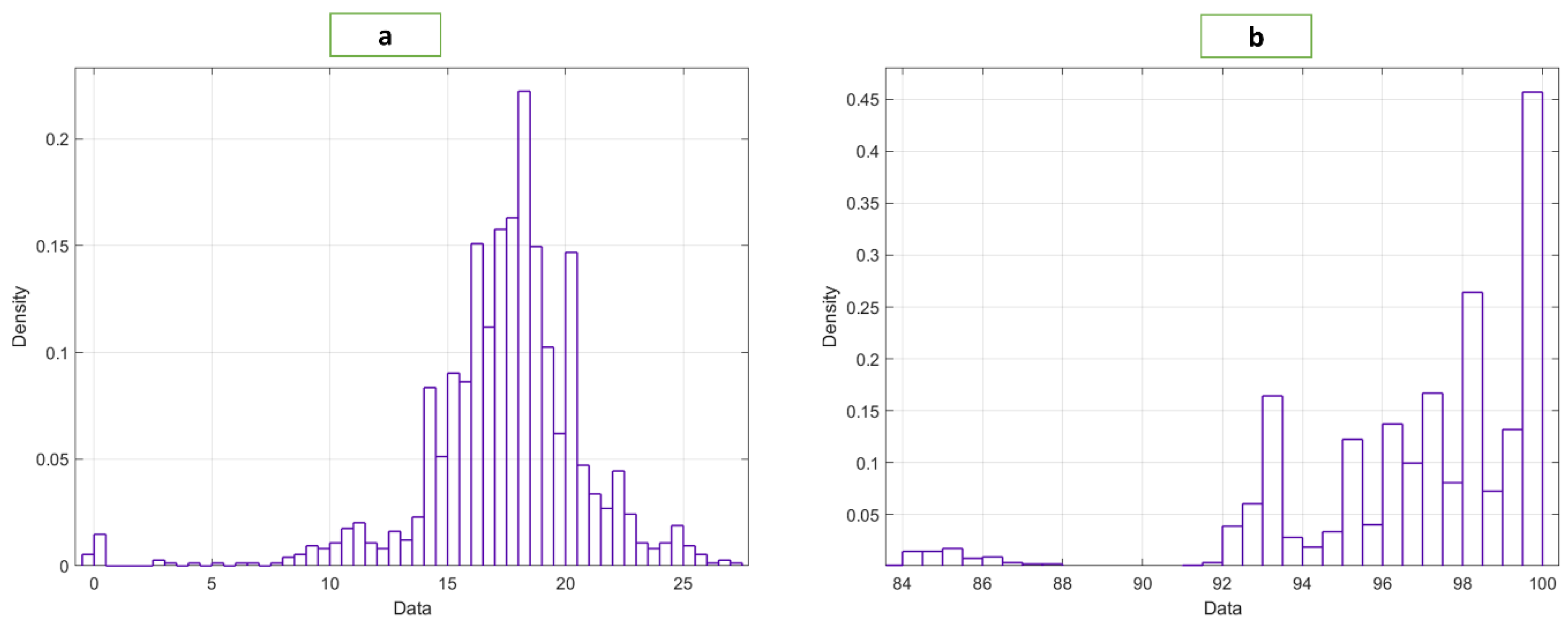
2.2. Preprocessing
2.3. Feature Extraction
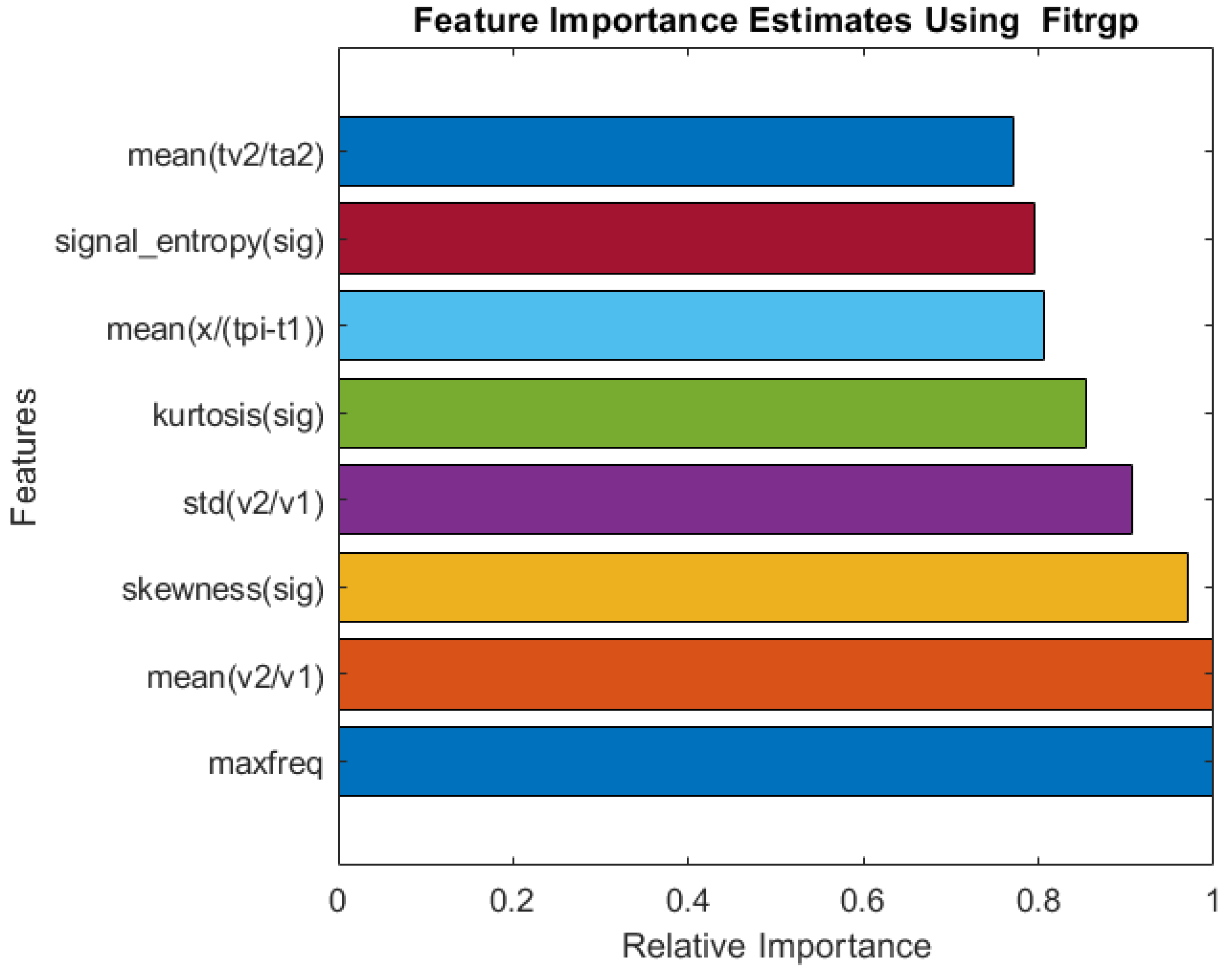
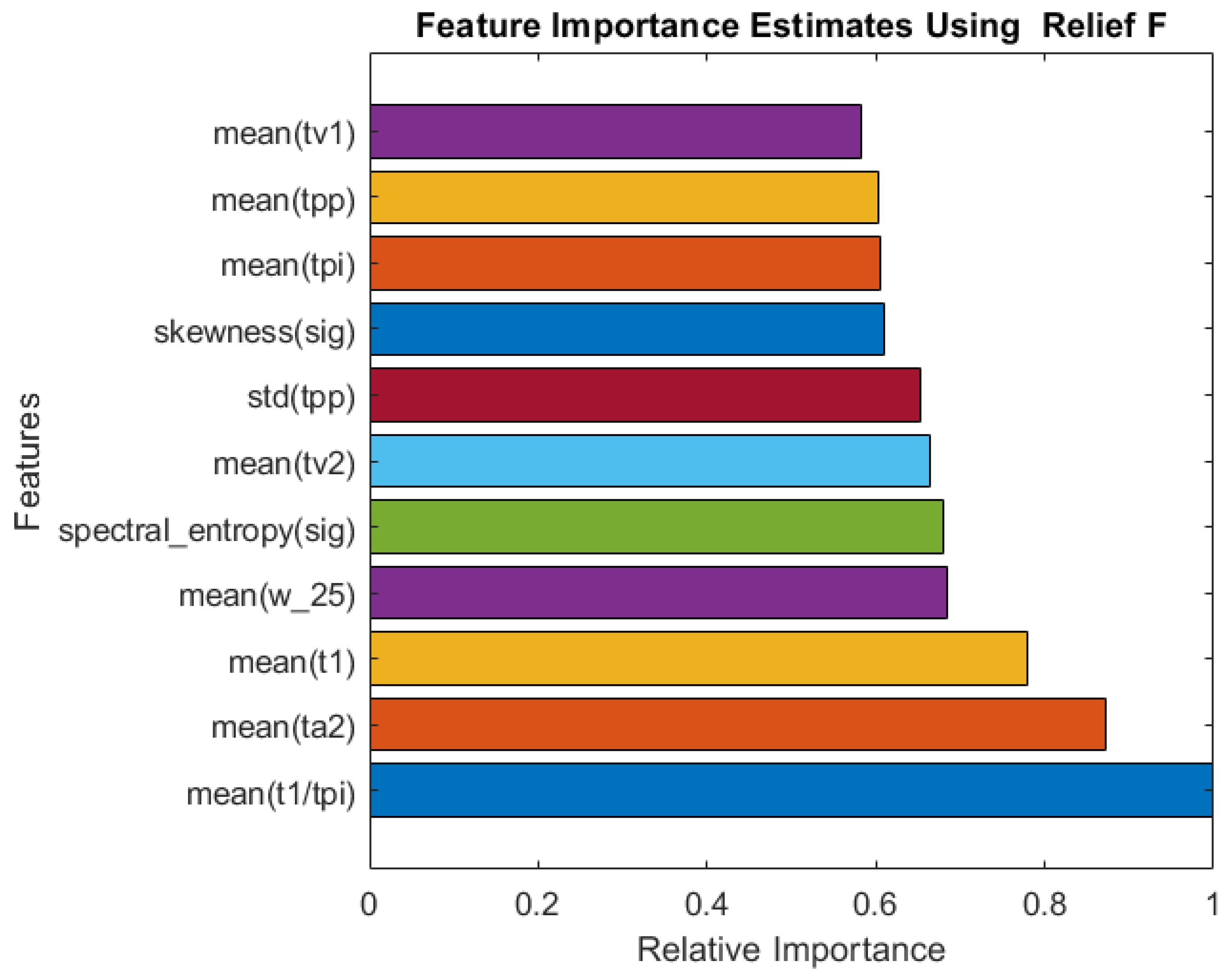
2.4. Feature Selection
2.5. Machine Learning
2.6. Evaluation Criteria
3. Results and Discussion
4. Conclusions
Supplementary Materials
Author Contributions
Funding
Institutional Review Board Statement
Informed Consent Statement
Data Availability Statement
Conflicts of Interest
References
- WHO Coronavirus (COVID-19) Dashboard|WHO Coronavirus (COVID-19) Dashboard with Vaccination Data. Available online: https://covid19.who.int/ (accessed on 22 August 2021).
- Vital Signs. Available online: https://my.clevelandclinic.org/health/articles/10881-vital-signs (accessed on 22 August 2021).
- Charlton, P.H.; Birrenkott, D.A.; Bonnici, T.; Pimentel, M.A.F.; Johnson, A.E.W.; Alastruey, J.; Tarassenko, L.; Watkinson, P.J.; Beale, R.; Clifton, D.A. Breathing Rate Estimation From the Electrocardiogram and Photoplethysmogram: A Review. IEEE Rev. Biomed. Eng. 2018, 11, 2–20. [Google Scholar] [CrossRef] [PubMed] [Green Version]
- Charlton, P.H.; Bonnici, T.; Tarassenko, L.; Clifton, D.A.; Beale, R.; Watkinson, P.J. An assessment of algorithms to estimate respiratory rate from the electrocardiogram and photoplethysmogram. Physiol. Meas. 2016, 37, 610–626. [Google Scholar] [CrossRef] [PubMed]
- Charlton, P.H.; Bonnici, T.; Tarassenko, L.; Alastruey, J.; Clifton, D.A.; Beale, R.; Watkinson, P.J. Extraction of respiratory signals from the electrocardiogram and photoplethysmogram: Technical and physiological determinants. Physiol. Meas. 2017, 38, 669–690. [Google Scholar] [CrossRef] [PubMed]
- Shah, S.A.; Fleming, S.; Thompson, M.; Tarassenko, L. Respiratory rate estimation during triage of children in hospitals. J. Med. Eng. Technol. 2015, 39, 514–524. [Google Scholar] [CrossRef]
- Zhang, X.; Ding, Q. Respiratory rate estimation from the photoplethysmogram via joint sparse signal reconstruction and spectra fusion. Biomed. Signal Process. Control 2017, 35, 1–7. [Google Scholar] [CrossRef]
- Motin, M.A.; Karmakar, C.K.; Kumar, D.K.; Palaniswami, M. PPG Derived Respiratory Rate Estimation in Daily Living Conditions. In Proceedings of the Annual International Conference of the IEEE Engineering in Medicine and Biology Society, EMBS 2020, Montreal, QC, Canada, 20–24 July 2020; pp. 2736–2739. [Google Scholar] [CrossRef]
- Motin, M.A.; Karmakar, C.K.; Palaniswami, M. Selection of Empirical Mode Decomposition Techniques for Extracting Breathing Rate From PPG. IEEE Signal Process. Lett. 2019, 26, 592–596. [Google Scholar] [CrossRef]
- L’Her, E.; N’Guyen, Q.-T.; Pateau, V.; Bodenes, L.; Lellouche, F. Photoplethysmographic determination of the respiratory rate in acutely ill patients: Validation of a new algorithm and implementation into a biomedical device. Ann. Intensiv. Care 2019, 9, 11. [Google Scholar] [CrossRef] [PubMed] [Green Version]
- Pirhonen, M.; Peltokangas, M.; Vehkaoja, A. Acquiring Respiration Rate from Photoplethysmographic Signal by Recursive Bayesian Tracking of Intrinsic Modes in Time-Frequency Spectra. Sensors 2018, 18, 1693. [Google Scholar] [CrossRef] [PubMed] [Green Version]
- Jarchi, D.; Rodgers, S.J.; Tarassenko, L.; Clifton, D.A. Accelerometry-Based Estimation of Respiratory Rate for Post-Intensive Care Patient Monitoring. IEEE Sens. J. 2018, 18, 4981–4989. [Google Scholar] [CrossRef]
- Hartmann, V.; Liu, H.; Chen, F.; Hong, W.; Hughes, S.; Zheng, D. Toward Accurate Extraction of Respiratory Frequency from the Photoplethysmogram: Effect of Measurement Site. Front. Physiol. 2019, 10, 732. [Google Scholar] [CrossRef]
- Luguern, D.; Perche, S.; Benezeth, Y.; Moser, V.; Andrea Dunbar, L.; Braun, F.; Lemkaddem, A.; Nakamura, K.; Gomez, R.; Dubois, J. An Assessment of Algorithms to Estimate Respiratory Rate from the Remote Photoplethysmogram. In Proceedings of the IEEE/CVF Conference on Computer Vision and Pattern Recognition Workshops, Seattle, WA, USA, 14–19 June 2020; pp. 1232–1241. [Google Scholar]
- Venkat, S.; Arsath P.S., M.T.; Alex, A.; S.P., P.; Balamugesh; D.J., C.; Joseph, J.; Sivaprakasam, M. Machine Learning Based SpO2 Computation Using Reflectance Pulse Oximetry. In Proceedings of the Annual International Conference of the IEEE Engineering in Medicine and Biology Society, EMBS 2019, Berlin, Germany, 23–27 July 2019; pp. 482–485. [Google Scholar] [CrossRef]
- Priem, G.; Martinez, C.; Bodinier, Q.; Carrault, G. Clinical Grade SpO2 Prediction through Semi-Supervised Learning. In Proceedings of the IEEE 20th International Conference on Bioinformatics and Bioengineering, BIBE 2020, Cincinnati, OH, USA, 26–28 October 2020; pp. 914–921. [Google Scholar] [CrossRef]
- BiOSENCY BORA Band SpO2 Validation Study—Full Text View—ClinicalTrials.Gov. Available online: https://clinicaltrials.gov/ct2/show/NCT03918018 (accessed on 22 August 2021).
- Vijayarangan, S.; Suresh, P.; Sp, P.; Joseph, J.; Sivaprakasam, M. Robust Modelling of Reflectance Pulse Oximetry for SpO2 Estimation. In Proceedings of the Annual International Conference of the IEEE Engineering in Medicine and Biology Society, EMBS 2020, Montreal, QC, Canada, 20–24 July 2020; pp. 374–377. [Google Scholar] [CrossRef]
- Saeed, M.; Villarroel, M.C.; Reisner, A.T.; Clifford, G.D.; Lehman, L.-W.H.; Moody, G.B.; Heldt, T.; Kyaw, T.H.; Moody, B.E.; Mark, R.G. Multiparameter Intelligent Monitoring in Intensive Care II: A public-access intensive care unit database. Crit. Care Med. 2011, 39, 952–960. [Google Scholar] [CrossRef] [PubMed] [Green Version]
- Pimentel, M.A.F.; Johnson, A.E.W.; Charlton, P.H.; Birrenkott, D.; Watkinson, P.J.; Tarassenko, L.; Clifton, D.A. Toward a Robust Estimation of Respiratory Rate From Pulse Oximeters. IEEE Trans. Biomed. Eng. 2017, 64, 1914–1923. [Google Scholar] [CrossRef]
- Shuzan, M.N.I.; Chowdhury, M.H.; Hossain, M.S.; Chowdhury, M.E.H.; Reaz, M.B.I.; Uddin, M.M.; Khandakar, A.; Mahbub, Z.B.; Ali, S.H.M. A Novel Non-Invasive Estimation of Respiration Rate from Motion Corrupted Photo-plethysmograph Signal Using Machine Learning Model. IEEE Access 2021, 9, 96775–96790. [Google Scholar] [CrossRef]
- Chowdhury, M.H.; Shuzan, N.I.; Chowdhury, M.E.; Mahbub, Z.B.; Uddin, M.M.; Khandakar, A.; Reaz, M.B.I. Estimating Blood Pressure from the Photoplethysmogram Signal and Demographic Features Using Machine Learning Techniques. Sensors 2020, 20, 3127. [Google Scholar] [CrossRef]
- Roffo, G. Feature Selection Library (MATLAB Toolbox). arXiv 2016, preprint. arXiv:1607.01327. [Google Scholar]
- Rasmussen, C.E. Gaussian Processes in Machine Learning; Lecture Notes in Computer Science (including subseries Lecture Notes in Artificial Intelligence and Lecture Notes in Bioinformatics); Springer: Berlin/Heidelberg, Germany, 2004; Volume 3176, pp. 63–71. [Google Scholar] [CrossRef] [Green Version]
- Lagarias, J.C.; Reeds, J.A.; Wright, M.H.; Wright, P.E. Convergence Properties of the Nelder—Mead Simplex Method in Low Dimensions. SIAM J. Optim. 1998, 9, 112–147. [Google Scholar] [CrossRef]
- Liu, H.; Motoda, H. (Eds.) Computational Methods of Feature Selection, 1st ed.; Chapman and Hall/CRC: Boca Raton, FL, USA, 2007; ISBN 9781584888789. [Google Scholar]
- Kononenko, I.; Šimec, E.; Robnik-Šikonja, M. Overcoming the Myopia of Inductive Learning Algorithms with RELIEFF. Appl. Intell. 1997, 7, 39–55. [Google Scholar] [CrossRef]
- Robnik-Šikonja, M.; Kononenko, I. Theoretical and Empirical Analysis of ReliefF and RReliefF. Mach. Learn. 2003, 53, 23–69. [Google Scholar] [CrossRef] [Green Version]
- Du, L.; Shen, Y.D. Unsupervised Feature Selection with Adaptive Structure Learning. In Proceedings of the ACM SIGKDD International Conference on Knowledge Discovery and Data Mining, Sydney, NSW, Australia, 10–13 August 2015; Association for Computing Machinery: New York, NY, USA; Volume 2015-Augus, pp. 209–218. [Google Scholar]
- Guo, J.; Quo, Y.; Kong, X.; He, R. Unsupervised Feature Selection with Ordinal Locality. In Proceedings of the IEEE International Conference on Multimedia and Expo, Hong Kong, China, 10–14 July 2017; IEEE Computer Society: New York, NY, USA, 28 August 2017; pp. 1213–1218. [Google Scholar]
- He, X.; Cai, D.; Niyogi, P. Laplacian Score for Feature Selection. Adv. Neural Inf. Process. Syst. 2005, 18, 507–514. [Google Scholar]
- Cristani, M.; Roffo, G.; Segalin, C.; Bazzani, L.; Vinciarelli, A.; Murino, V. Conversationally-Inspired Stylometric Features for Authorship Attribution in Instant Messaging. In Proceedings of the 20th ACM International Conference on Multimedia 2012, MM 2012, Nara, Japan, 2 November 2012; pp. 1121–1124. [Google Scholar] [CrossRef]
- Guyon, I.; Weston, J.; Barnhill, S.; Vapnik, V. Gene Selection for Cancer Classification using Support Vector Machines. Mach. Learn. 2002, 46, 389–422. [Google Scholar] [CrossRef]
- Bradley, P.S.; Mangasarian, O.L. Feature Selection via Concave Minimization and Support Vector Machines. ICML 1998, 98, 82–90. [Google Scholar]
- Framework for Ensemble Learning—MATLAB & Simulink. Available online: https://www.mathworks.com/help/stats/framework-for-ensemble-learning.html (accessed on 22 August 2021).
- Support Vector Machine Regression—MATLAB & Simulink. Available online: https://www.mathworks.com/help/stats/support-vector-machine-regression.html (accessed on 22 August 2021).
- Decision Trees—Scikit-Learn 0.24.2 Documentation. Available online: https://scikit-learn.org/stable/modules/tree (accessed on 22 August 2021).
- Linear Regression—MATLAB & Simulink. Available online: https://www.mathworks.com/help/matlab/data_analysis/linear-regression.html (accessed on 22 August 2021).
- Zhang, Q.; Arney, D.; Goldman, J.M.; Isselbacher, E.M.; Armoundas, A.A. Design Implementation and Evaluation of a Mobile Continuous Blood Oxygen Saturation Monitoring System. Sensors 2020, 20, 6581. [Google Scholar] [CrossRef] [PubMed]


| Selection Criteria | Top Features | Performance Criteria | GPR | Ensemble Tree | SVR | Decision Tree | Linear Regression |
|---|---|---|---|---|---|---|---|
| All Features | All | RMSE MAE | 1.45 1.00 | 1.61 1.00 | 2.04 1.27 | 2.09 1.27 | 3.04 1.86 |
| CFS | Top 28 Features | RMSE MAE | 1.60 1.02 | 1.74 1.15 | 7.66 2.30 | 2.18 1.36 | 6.58 2.27 |
| FSV | Top 30 Features | RMSE MAE | 1.47 0.91 | 1.61 0.98 | 3.58 2.40 | 2.06 1.23 | 3.45 2.09 |
| LASSO | Top 22 Features | RMSE MAE | 1.43 0.90 | 1.69 1.06 | 1.98 1.19 | 1.98 1.23 | 2.63 1.99 |
| Fitrgp | Top 8 Features | RMSE MAE | 1.41 0.89 | 1.72 1.11 | 1.62 0.97 | 2.06 1.22 | 2.89 2.08 |
| ReliefF | Top 30 Features | RMSE MAE | 1.51 0.99 | 1.66 1.04 | 2.10 1.26 | 1.94 1.19 | 2.71 2.04 |
| Ufsol | Top 19 Features | RMSE MAE | 1.50 0.94 | 1.76 1.10 | 1.90 1.12 | 2.16 1.33 | 2.74 2.03 |
| Llcfs | Top 23 Features | RMSE MAE | 1.57 1.04 | 1.82 1.14 | 2.00 1.20 | 2.27 1.40 | 2.86 2.15 |
| Laplacian | Top 29 Features | RMSE MAE | 1.72 1.14 | 1.88 1.23 | 2.08 1.35 | 2.13 1.13 | 10.08 2.76 |
| Fsasl | Top 30 Features | RMSE MAE | 1.80 1.09 | 1.96 1.29 | 2.19 1.44 | 2.24 1.21 | 3.80 2.05 |
| Selection Criteria | Top Features | Performance Criteria | GPR | Ensemble Tree | SVR | Decision Tree | Linear Regression |
|---|---|---|---|---|---|---|---|
| All Features | All | RMSE MAE | 1.23 0.73 | 1.41 0.80 | 1.91 1.27 | 1.83 0.92 | 3.51 1.80 |
| CFS | Top 28 Features | RMSE MAE | 1.43 0.96 | 1.64 1.11 | 5.66 2.19 | 2.03 1.21 | 5.58 2.04 |
| FSV | Top 30 Features | RMSE MAE | 1.38 0.87 | 1.50 0.82 | 3.40 2.28 | 1.98 1.12 | 3.25 2.00 |
| LASSO | Top 22 Features | RMSE MAE | 1.33 0.88 | 1.57 0.98 | 1.90 1.10 | 1.84 1.16 | 2.53 1.90 |
| Fitrgp | Top 18 Features | RMSE MAE | 1.00 0.59 | 1.51 0.88 | 1.76 0.96 | 1.76 0.79 | 2.36 1.61 |
| ReliefF | Top 11 Features | RMSE MAE | 0.98 0.57 | 1.49 1.87 | 1.68 0.86 | 1.19 0.81 | 3.02 2.41 |
| Ufsol | Top 19 Features | RMSE MAE | 1.39 0.90 | 1.61 0.99 | 1.77 1.01 | 2.06 1.21 | 2.62 1.97 |
| Llcfs | Top 23 Features | RMSE MAE | 1.47 0.98 | 1.72 1.04 | 1.92 1.08 | 2.17 1.33 | 2.66 2.01 |
| Laplacian | Top 29 Features | RMSE MAE | 1.62 1.08 | 1.78 1.11 | 1.97 1.25 | 2.03 1.05 | 6.80 1.67 |
| Fsasl | Top 30 Features | RMSE MAE | 1.63 0.96 | 1.76 1.07 | 2.11 1.24 | 2.11 1.13 | 3.03 1.95 |
| Author | Year | Database | Subject | Method | Metric | Result |
|---|---|---|---|---|---|---|
| Pirhonen et al. [11] | 2018 | Vortal | 39 Subjects | Wavelet Synchro—squeezing Transform | MAE RMSE R 2SD | 2.33 3.68 - - |
| Jarchi et al. [12] | 2018 | BIDMC | 10 Subjects | Accelerometer | MAE RMSE R 2SD | 2.56 - - - |
| Motin et al. [8] | 2019 | MIMIC II | 53 Subjects | Empirical Mode Decomposition | MAE RMSE R 2SD | 0–5.03 - - - |
| L’Her et al. [10] | 2019 | Own | 30 Subjects | Own Approach | MAE RMSE R 2SD | - - 0.78 - |
| Motin et al. [9] | 2020 | Own | 10 Subjects | Empirical Mode Decomposition | MAE RMSE R 2SD | 3.05 - - - |
| Shuzan et al. [21] | 2021 | Vortal | 39 Subjects | Machine Learning | MAE RMSE R 2SD | 1.97 2.63 0.88 5.25 |
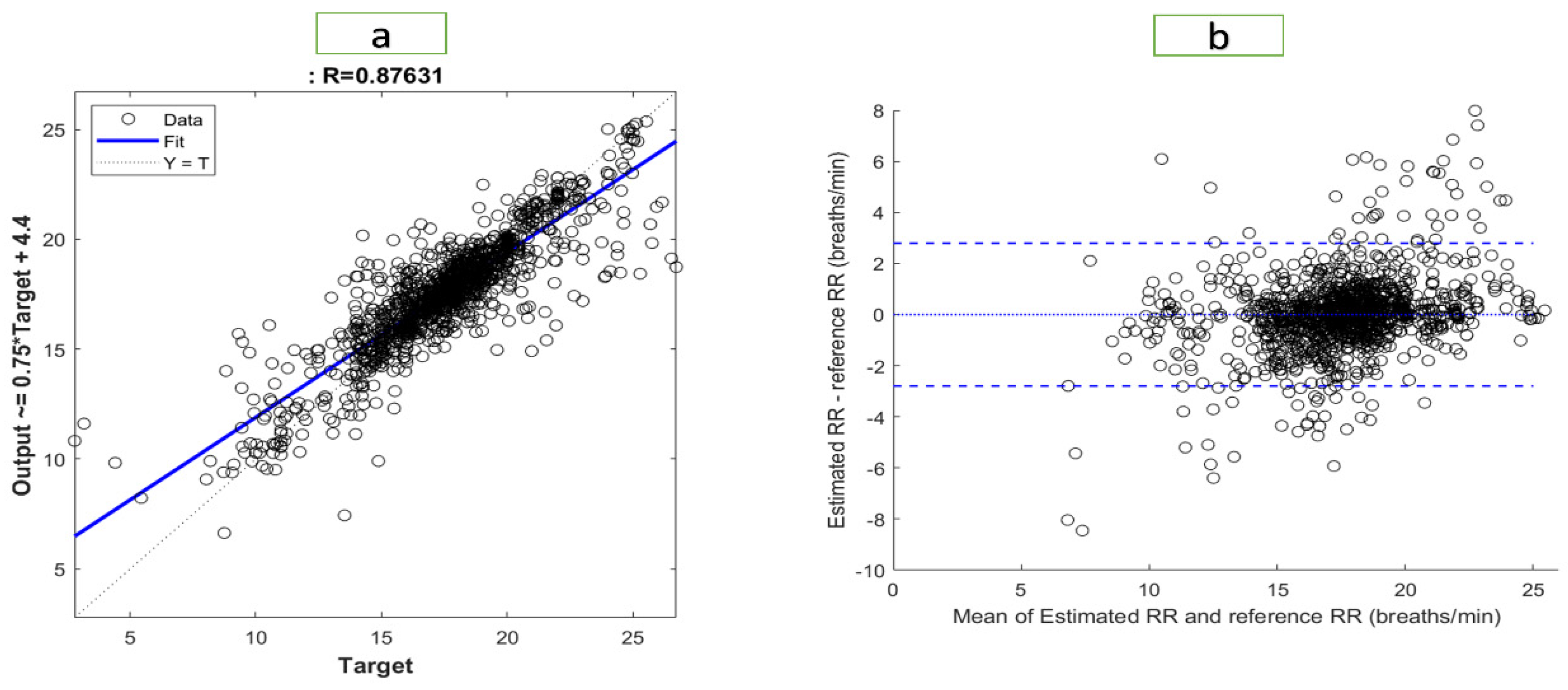
| This Work | 2021 | BIDMC | 53 Subjects | Machine Learning | MAE RMSE R 2SD | 0.89 1.41 0.87 2.83 |
| Author | Year | Database | Subject | SpO2 Range | Method | Metric | Result |
|---|---|---|---|---|---|---|---|
| Venkat et al. [15] | 2019 | Own | 95 subjects | 81–100% | Machine Learning | MAE RMSE R 2SD LOA | - - 0.95 - −2.12 to 2.12 |
| Priem et al. [16] | 2020 | Own | 10 subjects | 70–100% | Deep Neural Network | MAE RMSE R 2SD LOA | - 2.91 - - - |
| Zhang et al. [39] | 2020 | Own | 11 subjects | 95–100% | Own Approach | MAE RMSE R 2SD LOA | - 1.80 - - - |
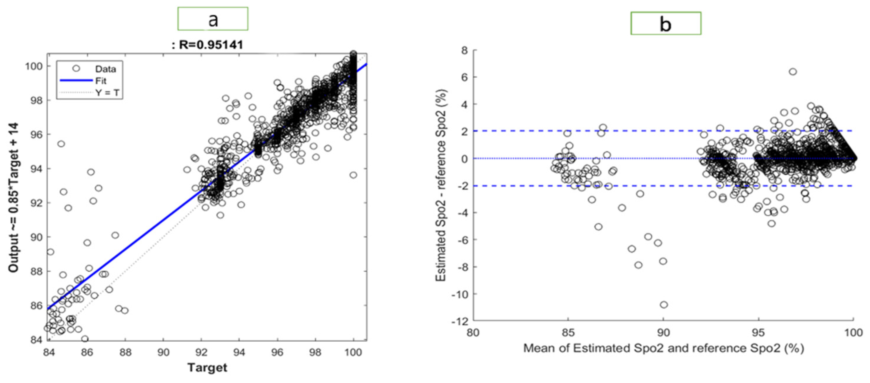
| Our Work | 2021 | BIDMC | 53 subjects | 85–100% | Machine Learning | MAE RMSE R 2SD LOA | 0.57 0.98 0.95 2.06 −2.04 to 2.03 |
| MAE (%) | RMSE (%) | SpO2 | ||
|---|---|---|---|---|
| Standard [17] | SpO2 | ≤2 | ≤3.5 | 70–100% |
| This paper | SpO2 | 0.57 | 0.98 | 84–100% |
Disclaimer/Publisher’s Note: The statements, opinions and data contained in all publications are solely those of the individual author(s) and contributor(s) and not of MDPI and/or the editor(s). MDPI and/or the editor(s) disclaim responsibility for any injury to people or property resulting from any ideas, methods, instructions or products referred to in the content. |
© 2023 by the authors. Licensee MDPI, Basel, Switzerland. This article is an open access article distributed under the terms and conditions of the Creative Commons Attribution (CC BY) license (https://creativecommons.org/licenses/by/4.0/).
Share and Cite
Shuzan, M.N.I.; Chowdhury, M.H.; Chowdhury, M.E.H.; Murugappan, M.; Hoque Bhuiyan, E.; Arslane Ayari, M.; Khandakar, A. Machine Learning-Based Respiration Rate and Blood Oxygen Saturation Estimation Using Photoplethysmogram Signals. Bioengineering 2023, 10, 167. https://doi.org/10.3390/bioengineering10020167
Shuzan MNI, Chowdhury MH, Chowdhury MEH, Murugappan M, Hoque Bhuiyan E, Arslane Ayari M, Khandakar A. Machine Learning-Based Respiration Rate and Blood Oxygen Saturation Estimation Using Photoplethysmogram Signals. Bioengineering. 2023; 10(2):167. https://doi.org/10.3390/bioengineering10020167
Chicago/Turabian StyleShuzan, Md Nazmul Islam, Moajjem Hossain Chowdhury, Muhammad E. H. Chowdhury, Murugappan Murugappan, Enamul Hoque Bhuiyan, Mohamed Arslane Ayari, and Amith Khandakar. 2023. "Machine Learning-Based Respiration Rate and Blood Oxygen Saturation Estimation Using Photoplethysmogram Signals" Bioengineering 10, no. 2: 167. https://doi.org/10.3390/bioengineering10020167