Article

An Efficient Data Driven-Based Model for Prediction of the Total Sediment Load in Rivers

1
School of Environment, College of Engineering, University of Tehran, Tehran 1417853111, Iran
2
Faculty of Governance, University of Tehran, Tehran 1439814151, Iran
3
Department of Physics, Faculty of Science, Shiraz Branch, Islamic Azad University, Shiraz 7198774731, Iran
4
Civil Engineering Department, Faculty of Engineering, University of Bojnord, Bojnord 9453155111, Iran
5
School of Civil Engineering, Iran University of Science and Technology, Narmak, Tehran 1684613114, Iran
6
School of Engineering, University of Warwick, Coventry CV4 7AL, UK
*
Author to whom correspondence should be addressed.
Hydrology 2022, 9(2), 36; https://doi.org/10.3390/hydrology9020036
Submission received: 30 January 2022 / Revised: 14 February 2022 / Accepted: 14 February 2022 / Published: 17 February 2022

Abstract

:
Sediment load in fluvial systems is one of the critical factors shaping the river geomorphological and hydraulic characteristics. A detailed understanding of the total sediment load (TSL) is required for the protection of physical, environmental, and ecological functions of rivers. This study develops a robust methodological approach based on multiple linear regression (MLR) and support vector regression (SVR) models modified by principal component analysis (PCA) to predict the TSL in rivers. A database of sediment measurement from large-scale physical modelling tests with 4759 datapoints were used to develop the predictive model. A dimensional analysis was performed based on the literature, and ten dimensionless parameters were identified as the key drivers of the TSL in rivers. These drivers were converted to uncorrelated principal components to feed the MLR and SVR models (PCA-based MLR and PCA-based SVR models) developed within this study. A stepwise PCA-based MLR and a 10-fold PCA-based SVR model with different kernel-type functions were tuned to derive an accurate TSL predictive model. Our findings suggest that the PCA-based SVR model with the kernel-type radial basis function has the best predictive performance in terms of statistical error measures including the root-mean-square error normalized with the standard deviation (RMSE/StD) and the Nash–Sutcliffe coefficient of efficiency (NSE), for the estimation of the TSL in rivers. The PCA-based MLR and PCA-based SVR models, with an overall RMSE/StD of 0.45 and 0.35, respectively, outperform the existing well-established empirical formulae for TSL estimation. The analysis of the results confirms the robustness of the proposed PCA-based SVR model for prediction of the cases with high concentration of sediments (NSE = 0.68), where the existing sediment estimation models usually have poor performance.

1. Introduction

Natural and anthropogenically driven forces during the Anthropocene are threatening the sustainable function of rivers by introducing large sediment loads to the freshwater ecosystems and fluvial systems. Extreme total sediment load (TSL) in the rivers can threaten the aquatic life and impose negative impacts on the ecosystem’s health and function. Large TSL can clog the fish gills, limit the light penetration into the riverbed, decrease the photosynthesis of hydrophytes, change the riverbed with profound implications for benthic organisms, transport large pollution loads, and deplete the river dissolved oxygen content [1,2,3,4,5,6,7,8,9,10,11,12,13]. Additionally, the sediments could affect the river hydraulic and geometry by decreasing the cross-section dimension and the flow discharge capability, reducing the active storage available within the rivers, clogging bridges and culverts, and changing vegetation growth patterns that impacts roughness and ecosystem of rivers [6,8,14,15,16,17,18,19]. Thus, an accurate predictive capability of the TSL is required to understand the physical, environmental and ecological responses of the rivers to sediment load, and minimize the negative impacts of sediments on the river ecosystem.
The quantity of the TSL in fluvial systems is usually studied by two well-established approaches. The first approach studies the bed loads and suspended loads separately, as the components of the TSL [20,21,22], while the second approach quantifies the TSL by considering the combined effects of both the bed and suspended load components [23,24,25,26]. In general, the decision to choose one of the above approaches is based on a wide range of factors such as the available data, the accuracy needed for the design studies, and the riverbed type. For example, in gravel-bed rivers, the TSL is mainly transported as the bed load, whereas in sandy-bed rivers, both suspended and bed load phases contribute to the TSL [27]. Therefore, the decision on the appropriateness and robustness of the two described approaches for TSL quantification is complex, given that the addition of hydro-morphological factors to input–output relationships can introduce different levels of uncertainty in the outcomes of numerical models. Overall, the TSL model that considers both bed and suspended load components together has been widely used by researchers given that the detection and differentiation between the bed and suspended loading is not readily possible [23,24,25,26,28,29].
Several laboratory and field-based studies have been carried out to model the river sediment loads using dimensional variables such as flow rate and geometric characteristics of the riverbed [30,31,32,33,34]. In controlled laboratory flumes, a wide range of hydraulic and morphological variables can be modelled, enabling detailed analysis of the effects of different variables influencing the sediment transport, and derivation of empirical formulae for TSL estimation. In recent years, applications of advanced data driven and machine learning (ML) approaches have been explored to provide a more accurate estimation in hydrological applications, especially suspended loads [28,35,36,37,38,39,40,41]. However, due to the difficulty in measuring some of the effective parameters that influence the transport of sediments in rivers (hereafter referred to as “drivers”), the available empirical-based equations and data driven models for the estimation of TSL only rely on few easily measurable variables in rivers. Meanwhile, ignoring the main drivers of the TSL in rivers, can reduce the accuracy of the existing methods for predicting the sediment concentration in rivers. Therefore, a comprehensive review of the drivers of the TSL is necessary to derive more robust formulae for the estimation of the TSL for a range of hydro-environmental and geomorphological conditions. Another challenge associated with the existing empirical-based models is their applicability for extreme TSL conditions, given that such models are derived based on a limited range of sediment concentration in rivers [30]. Although empirical-based models provide reasonable accuracy for TSL estimation under the usual mild environmental conditions, the main concern is always associated with the extreme events that introduce high concentration of sediments into the rivers.
In this study, a dimensional analysis is carried out based on the literature to determine the main drivers of the TSL in rivers. Following dimensional analysis, two robust models are developed for estimation of the TSL, using multiple linear regression (MLR) and support vector regression (SVR) techniques modified by the principal component analysis (PCA) model (PCA-based MLR and PCA-based SVR models). Application of PCA on the main drivers of TSL in rivers can improve the predictive performance of MLR and SVR models by removing the dependency occurrence among inputs. Our modeling results suggest the robustness of the proposed PCA-based MLR and PCA-based SVR models for the prediction of the cases with high concentration of sediments, where the existing sediment estimation models usually have poor performance.

2. Materials and Methods

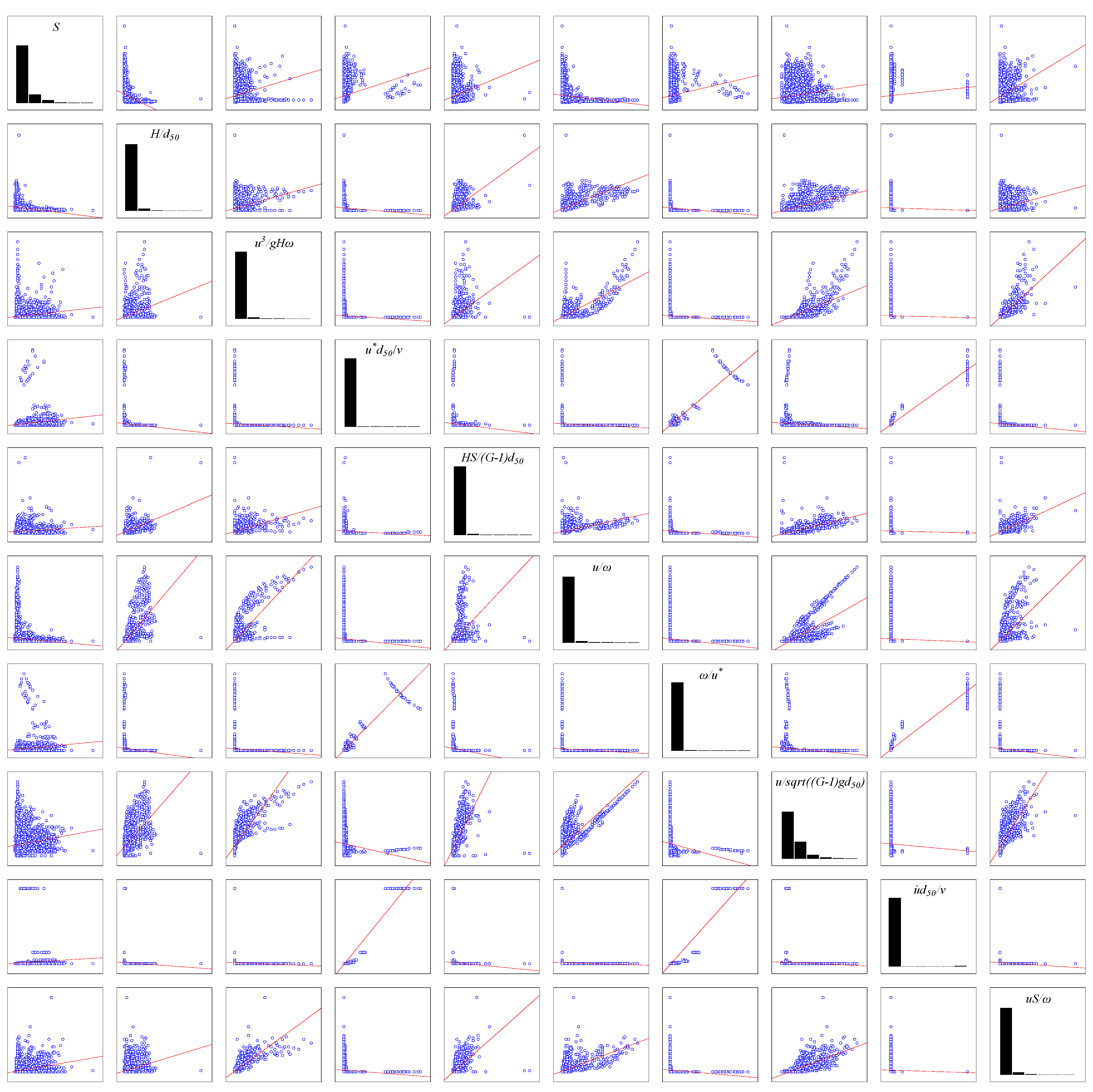
2.1. Dimensional Analysis
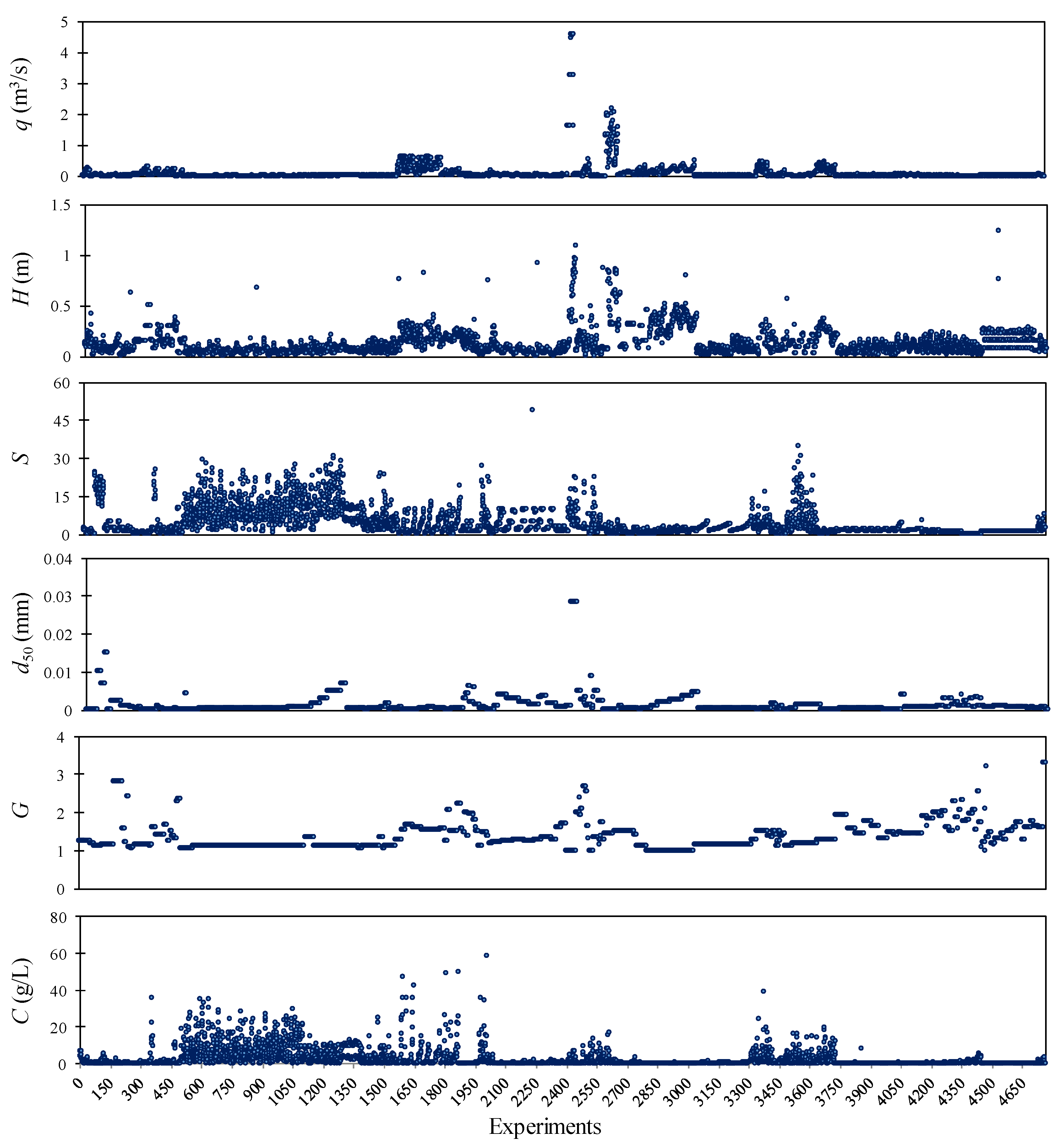
River flow properties, sediment load characteristics, and geometrical configurations are the main effective parameters determining the variation of TSL in rivers [23,24,42,43,44]. River flow properties include the flow rate (q), velocity (u), shear velocity (u*), flow depth (H), kinematic viscosity ( ϑ ), and flow temperature (T). The average particle diameter by mass (d50), sediment particle settling velocity (ω), and specific density of sediment particles (G) can be considered as the key sediment load characteristics. Literature suggests that the river longitudinal slope (S) is a key geometrical configuration that impacts the TSL in rivers [26]. Mathematically, the concentration of sediments in rivers C, can be described by Equation (1):
C = ʘ ( q , u , u * , H , T , d 50 , G , S , ϑ , ω )
In Equation (1), the sediment particle’s settling velocity is determined as:
ω = 1 18 g ( S 1 ) d 50 2 ϑ
where, g is the gravitational acceleration constant.
The existing data-driven models for the estimation of the TSL in rivers have used different combinations of the parameters described in Equation (1), in both dimensional and dimensionless forms. A review of the literature suggests that the dimensionless parameters adopted in previous studies can be summarized as:
C = f ( S , H d 50 , u 3 g H ω , u * d 50 ϑ , H S ( G 1 ) d 50 , u ω , ω u * , u ( G 1 ) g d 50 , ω d 50 ϑ , u S ω )
Equation (3) described the ten main drivers of TSL which are used as predictors of sediment concentration in this study.

2.2. Database

This study adopts sediment measurement data from large-scale physical modelling tests. Database includes 4759 laboratory experiments performed by [25], including measurements of C, q, H, G, S, T, and d50 parameters, as the most effective factors contributing to the TSL in rivers. The flow velocity and shear velocity were calculated for the database as u = q / W (W is the flow width) and u * = g S H , respectively. The kinematic viscosity ϑ , was determined for all the data using the methodology proposed by [45] and T measurements. Figure 1 illustrates the variation of the parameters in the raw database used in this study. The statistical characteristics of the raw database was determined and presented in Table S1 and Supplementary Materials.

2.3. Development of the TSL Regression-Based Models

All the ten dimensionless drivers given in Equation (3) are considered as the predictors for development of the TSL regression-based predictive models. The literature suggests that these drivers have major influence on the TSL in rivers [23,24,42,43,44]. Following the standardized protocols for development of data-driven regression models, approximately 75% of the database (3569 datapoints) was used to calibrate the TSL regression models, and the remaining 1190 datapoints (25% of database) were used to verify the calibrated models.
Suppose P = { C i , x i ; i = 1 ,   , n } consists of the calibration datapoints, where the index i labels the n calibration datapoints (n = 3569), and C and x are the vectors of sediment concentration and the drivers of the TSL in rivers (Equation (3)), respectively. To develop the regression-based predictive models for TSL, the functional dependence of the sediment concentration C, on the drivers, i.e. x, should be estimated using calibration datapoints. The relationship between C and x can be described by a deterministic function as:
C = ( x ) + h
where, h is additive noise.
In this study, the functional form is explored to enable the accurate prediction of the verification datapoints (i.e., unseen data), such that the developed regression-based TSL models did not experience before. The functional form can be reached by tuning the developed models during the calibration process, and by considering a mechanism for optimization of the defined error function.

2.3.1. Development of PCA-Based MLR Model for TSL Prediction

MLR is a linear tool to model the relationship between a scalar response (known as a dependent variable) and multi-explanatory drivers (known as independent variables). Considering the database of P, the theory of the MLR supposes that the deterministic function can be represented as a linear relationship described by Equation (5):
C i = β 0 + β 1 x i 1 + β 2 x i 2 + + β r x i r + h i = x i T β + h i
where, r = 10 (the number of drivers), β is the vector of coefficients, superscript T denotes the transpose of a matrix or a vector, hi is supposed as an independent parameter with a Gaussian distribution [46].
In this study, there are n number of calibration datapoints (=3569 datapoints), leading to the formation of a system of 3569 linear equations described in a compact form by Equation (6).
C = X β + h
Refereeing to Equations (4) and (6), the deterministic function is defined as Xβ. Thus, the aim is to determine the vector β using the ordinary least square procedure in the MLR model. This can be carried out by the minimization of | | X β C 2 | | , which is also known as the Euclidean norm of the error function. Finally, the regression coefficient β can be determined as [46,47]:
β = ( X T X ) 1 ( X T C )
In the case of strong correlations among the exploratory drivers, inversion of matrix X T X introduces a large error to the tuned MLR model [48]. To address this problem in the calibration dataset, the PCA method was applied to remove multicollinearity between the drivers. The PCA method converts the drivers to new and uncorrelated principal components (PCs) [49,50]. These new uncorrelated inputs, i.e., PCs, can be used as independent variables for the MLR model (PCA-based MLR model) [46]. Variance inflation factor (VIF), as a universal criterion for the detection of multicollinearity in the MLR model, is adopted in this study [51]. The VIF varies from 1 to ∞, with the larger values corresponding to higher probability of multicollinearity occurrence in the input data. The VIF > 2 can usually be a sign of multicollinearity in the data; however, this study adopted the VIF > 10 as a condition that can introduce a significant error in the modeling process [46,52].

2.3.2. Development of PCA-Based SVR Model for TSL Prediction

SVR is a robust machine learning model for problems with complex nonlinear relationships between the input and output variables. The computational intricacies of the SVR model do not depend on the input space dimensionality [53]. Therefore, the SVR model has successfully been applied to river engineering problems, where multidimensional drivers impact the water quality in the rivers. However, the occurrence of a strong correlation between the independent variables can result in a poor prediction of the sediment concentration using the SVR model [54]. Adoption of PCA can help reduce the effects of dependency between the drivers. Therefore, this study replaced the ten influential drivers with the corresponding uncorrelated PCs as inputs to the SVR model (PCA-based SVR model).
The error function in the PCA-based SVR model is determined according to Equation (8):
τ T τ 2 + m ( i = 1 n ξ i + i = 1 n ξ i * )
where, τ is the vector of coefficients, m is the capacity constant, ξ i and ξ i * are slack variables that handle non-separable input data.
Here, Equation (8) should be minimized subject to the following constrains:
τ T ( P C i ) + b C i ε + ξ i *
C i τ T ( P C i ) b ε + ξ i *
ξ i , ξ i * 0 ;   i = 1 , , n
where, is the kernel-type function [55,56].
SVR model is capable of handling highly complex datasets using an efficient kernel-type function technique (here, k ( P C i , P C j ) ) that reorganizes the datasets for linear solution transformation [57,58]. In this study, the kernel-type function is used for transforming the input parameters, i.e., PCs, to the feature space. SVR models have the flexibility of using a range of kernel-type functions including linear-type (Equation (10)), polynomial-type (Equation (11)), sigmoid-type (Equation (12)), and radial basis function kernel, i.e., RBF-type (Equation (13)) [55,56].
k ( P C i , P C j ) = ( P C i . P C j )
k ( P C i , P C j ) = ( P C i . P C j ) l
k ( P C i , P C j ) = tanh ( k P C i . P C j + α )
k ( P C i , P C j ) = exp ( γ P C i P C j 2 ) ;   γ > 0
In this study, we examined the performance of the developed PCA-based SVR model with different kernel-type functions to propose an accurate and robust TSL estimation model for rivers based on the ten uncorrelated PCs obtained from the conversion of the highly influential drivers given in Equation (3). The PCs and output variable C were first ranged from −1 to 1, and consequently fed to the developed SVR model. A two-step grid search algorithm is implemented to tune the PCA-based SVR model. Detailed information on the kernel-type functions and two-step grid search algorithm are given by [54,59].

2.4. Statistical Measures

The Nash–Sutcliffe coefficient of efficiency (NSE) index (Equation (14)) [60] and the root-mean-square error (RMSE) (Equation (15)) are used to evaluate the performance of the developed models:
NSE = 1 i = 1 n ( C i C ´ i ) 2 i = 1 n ( C i C ¯ i ) 2
RMSE = i = 1 n ( C ´ i C i ) 2 n
where, C i and C ´ i , in our study, are measured and predicted sediment concentration, respectively, and C ¯ i is the average value of the measured sediment concentration in the database. The perfect model has closer NSE and RMSE values to one (1) and zero (0), respectively [60,61].
However, RMSE defines the deviation of the model outputs from the observations in the units of the used variable. Therefore, normalizing the RMSE with a statistic that describes the range of the used variable, such as standard deviation (StD), can help the readers to better judge the model’s performance. In this regard, [13,19] concluded that RMSE values smaller than half of the standard deviation of the observations are acceptable for the evaluation of a model. Here, we use the NSE and RMSE/StD to evaluate the performance of the developed PCA-based MLR and PCA-based SVR models.

3. Results and Discussion

3.1. Pre-Processing Data Using PCA

Figure 2 shows the results of the dependence test for the ten input parameters used in this study. The results suggest a significant dependency (correlation coefficient > 0.6) between some of the drivers (e.g., u/ω and H/d50, u3/gHω and u/(sqrt(G−1)gd50), u/ω and u3/gHω, ω/u* and ωd50/v, u*d50/v and ωd50/v, and u3/gHω and uS/ω). These strong correlations can break down the independent condition between the drivers, leading to multicollinearity problems in fitting the TSL regression models and interpretation of the results. Additionally, high correlation between the drivers hinders the generalization performance of the ML models such as SVR [62].
To apply the PCA to the drivers, a symmetrical correlation matrix was created (Table S2). The matrix’s eigenvalues and their corresponding eigenvectors were determined. Statistical analysis shows KMO (Kaiser/Meyer/Olkin) = 0.72, where KMO values larger than 0.5 denote the suitability of a database for PCA implementation [46,63]. Bartlett’s sphericity statistical test was conducted to understand the redundancy amongst the input parameters, and further confirm the appropriateness of using PCA for the database investigated in this study [46]. Following the statistical evaluations, the ten uncorrelated PCs corresponding to the drivers were determined using the PCA application (Figures S1–S10). Table 1 shows the general characteristics of each PC determined for the input parameters, where the first PC (i.e., PC1) with more than 42% conservation of the drivers’ variance is the most important component. The larger index of “s” in the PCs, can be translated to less importance of that PC in conservation of the drivers’ variance. According to Table 1, the contribution of all PCs in conservation of the drivers’ variance reaches to 100%, indicating that the ten uncorrelated PCs can be used instead of the ten drivers in the development of the TSL regression models.

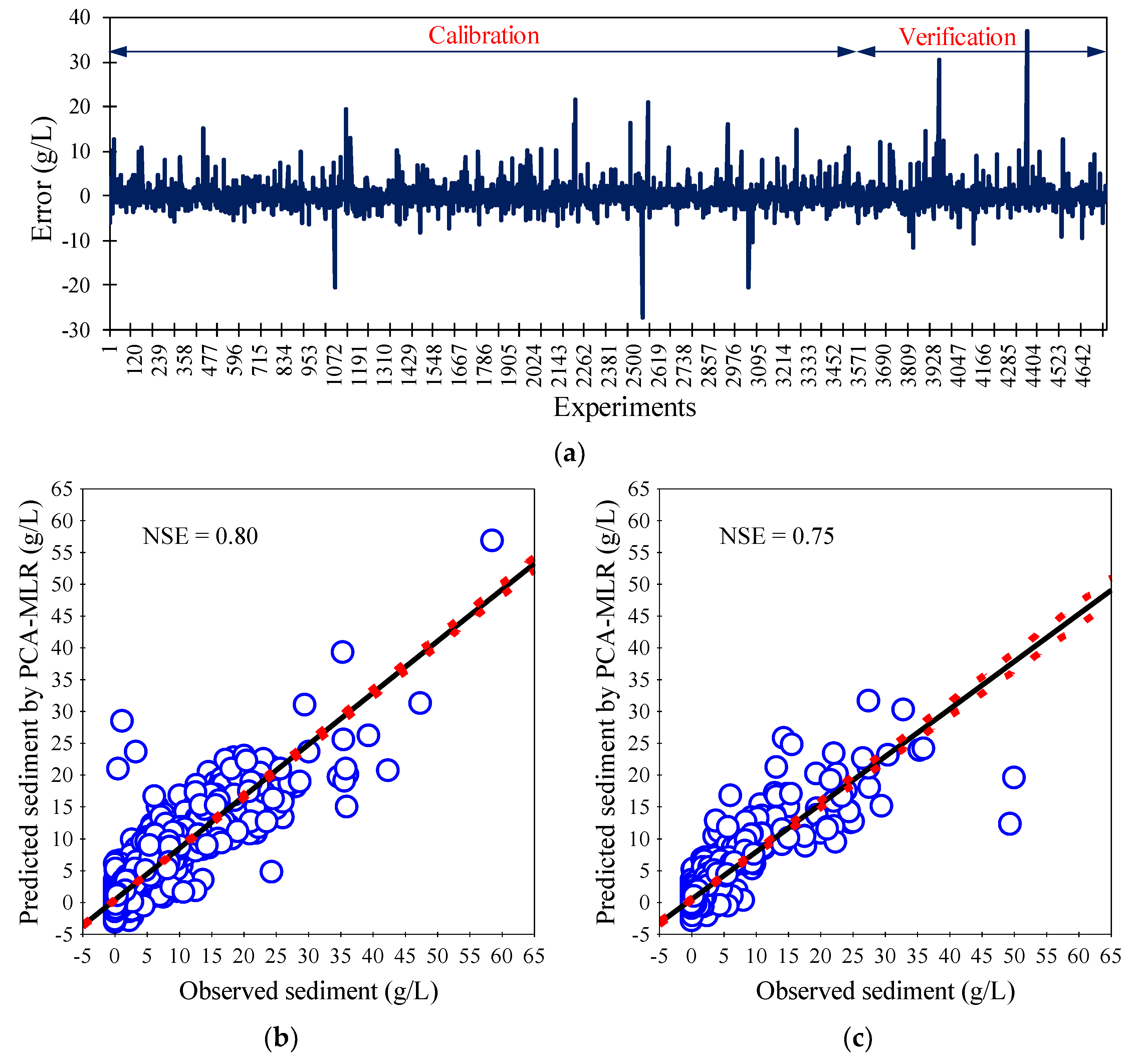
3.2. PCA-Based MLR Results

Following the computation of the uncorrelated PCs, the PCA-based MLR model was developed for TSL prediction in rivers, using a stepwise approach. In this regard, the PCA-based MLR model was constructed step by step, by addition of the potential PCs in succession until they can satisfy the statistical significance after each iteration. The results obtained suggest that all ten uncorrelated PCs satisfy the conditions required by the stepwise algorithm for the developed PCA-based MLR model (Table 2). The VIF values equal to 1 confirm no multicollinearity occurrence in the developed model. To better understand the impacts of strong dependency between drivers on the TSL regression model, the results of the developed MLR model with the ten raw drivers (Equation (3)) are also computed and presented in Table 2. The VIF values > 2 and especially those greater than 10 for some of the drivers (i.e., ω/u*, ωd50/v, and u*d50/v) denote the occurrence of multicollinearity in the developed MLR model that can lead to poor performance of the model. In addition, the stepwise algorithm has resulted in the exclusion of the HS/(G − 1)d50 parameter in the construction of the MLR model with the raw drivers. Meanwhile, HS/(G − 1)d50 parameter has been determined as a main driver used in other well-established sediment estimation equations [23].
Figure 3a shows the error between the sediment concentrations estimated by the PCA-based MLR model and those measured in laboratory flumes during both calibration and verification steps. The RMSE/StD (NSE) values for this model are 0.43 (0.81) and 0.48 (0.76) in the calibration and verifications steps, respectively (Figure 3b,c), denoting the acceptable accuracy of the model for the TSL prediction in rivers. However, the PCA-based MLR model is less accurate in the prediction of extreme sediment concentrations (Figure 3b,c). This can be related to the complex processes that govern the sediment transport in the rivers, influenced by a wide range of drivers that highly fluctuate in both time and space. Although this study includes the main drivers of the TSL in rivers, the effects of additional factors such as the river aspect ratio, friction term, and channel sinuosity, that may contribute to change in sediment concentration in rivers [64,65,66,67,68], are not considered in this study.

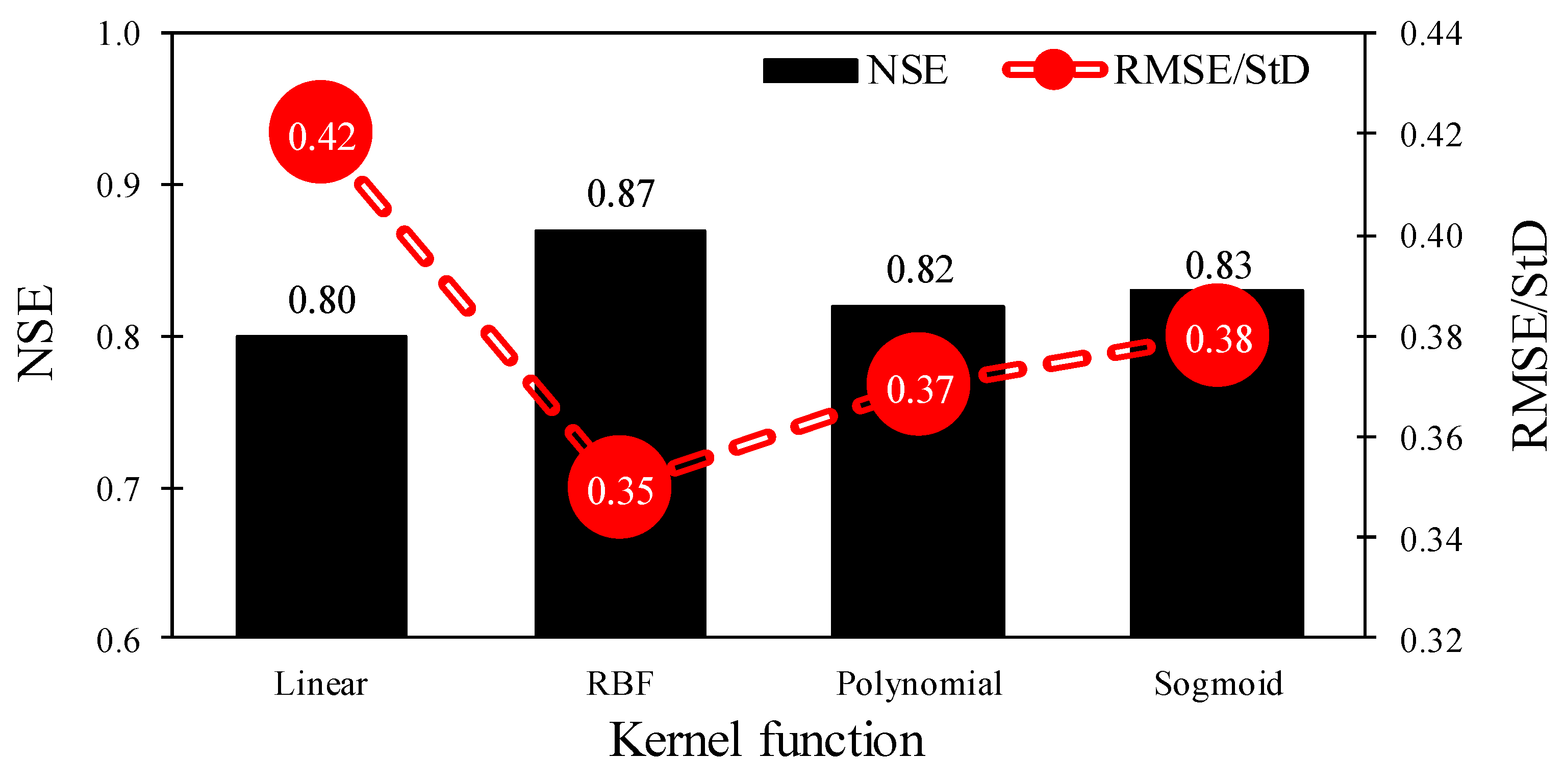
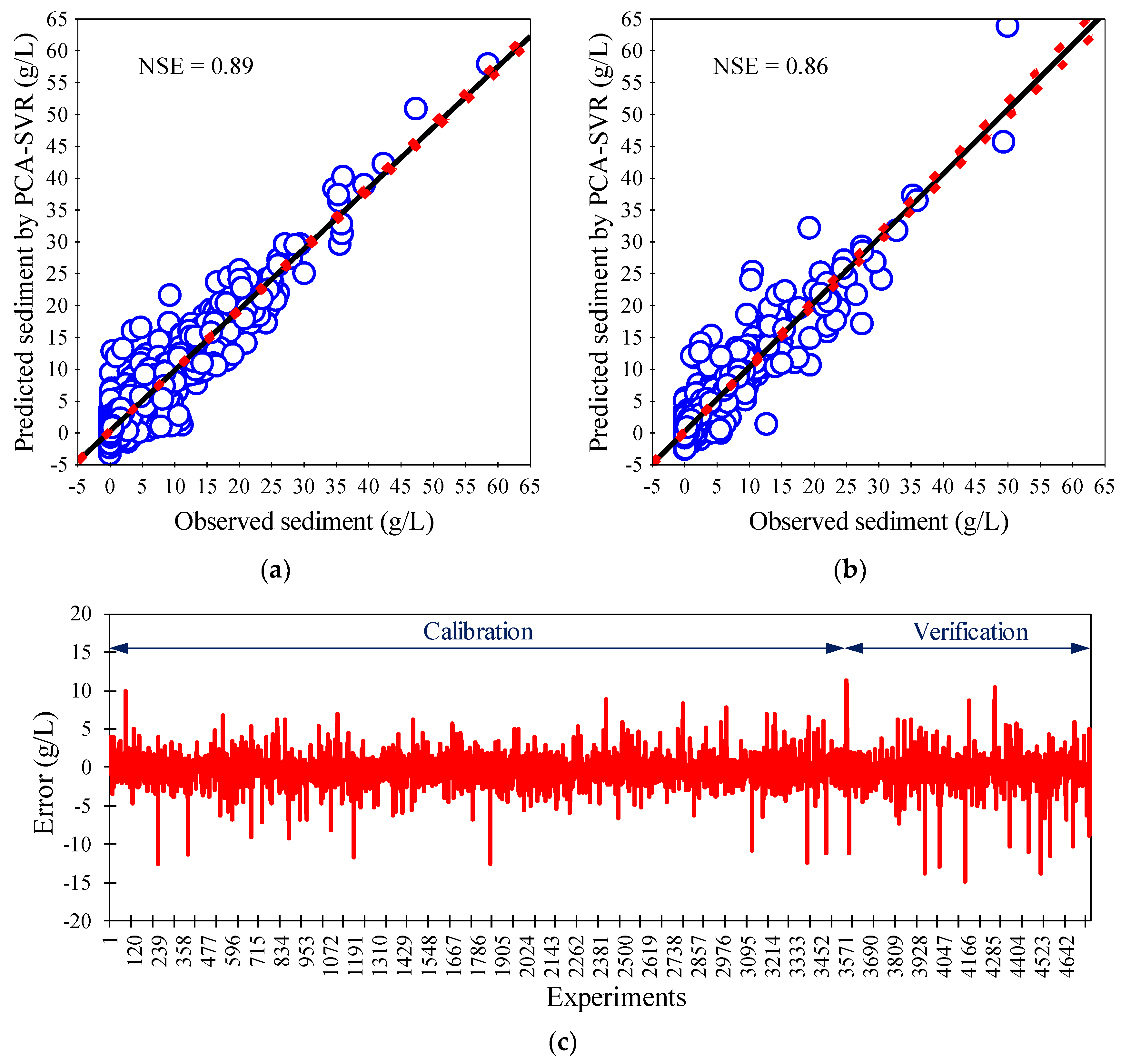
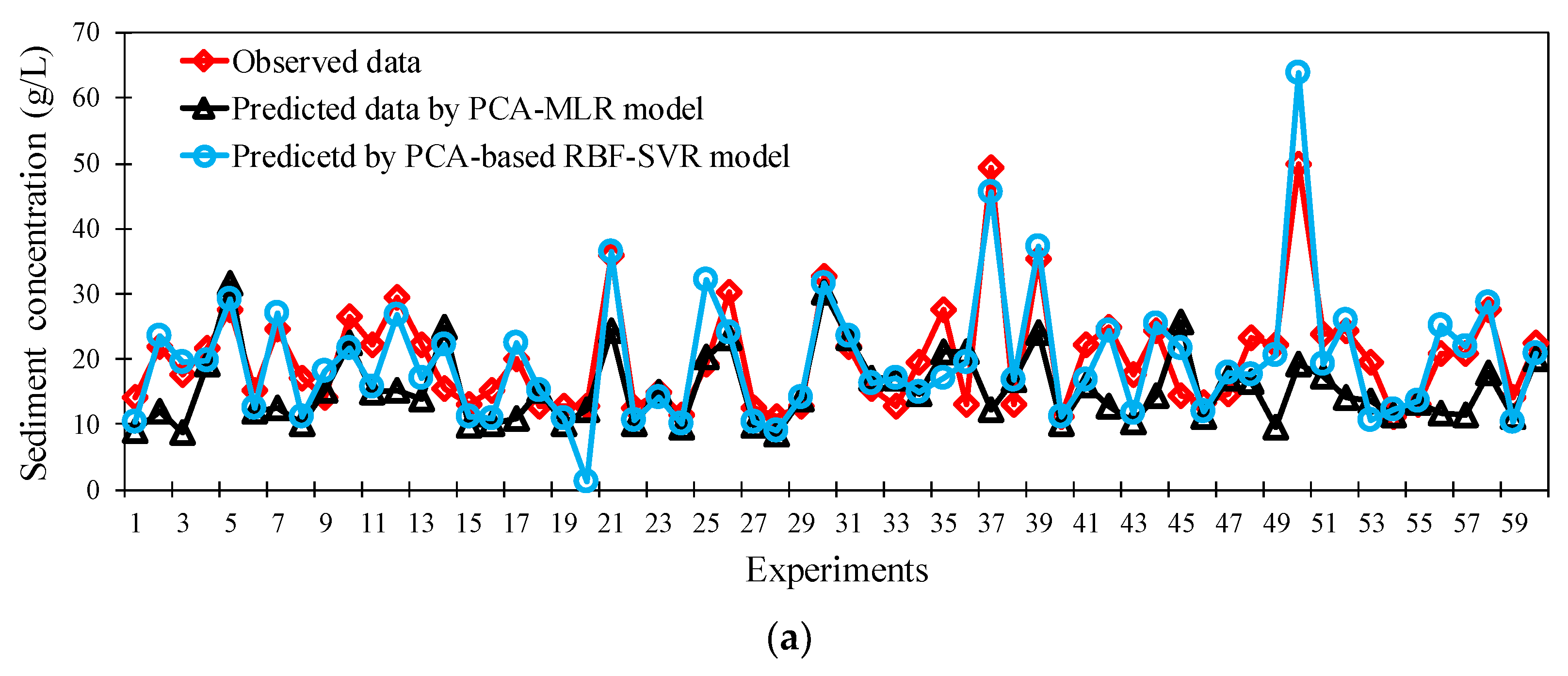
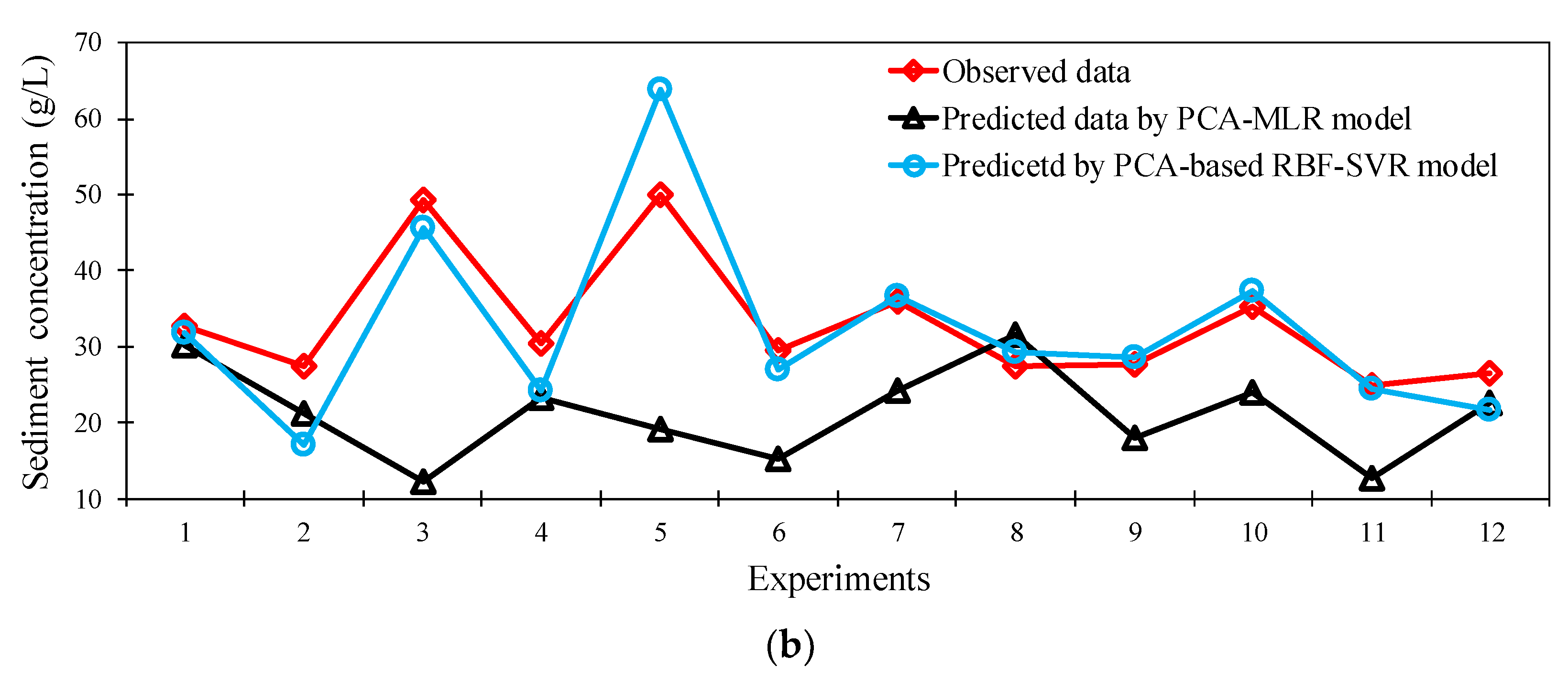
3.3. PCA-Based SVR Results

Similar to the MLR model development, ten uncorrelated PCs were fed to the SVR model (PCA-based SVR) for prediction of TSL in rivers. Then, a range of kernel-type functions were examined for the PCA-based SVR models. No optimization algorithm was used to drive the SVR model’s parameters during the kernel-type function evaluation process. Comparison of the prediction results for all the kernel-type functions tested within this study suggests that the SVR model with all the four kernel-types (Equations (10) and (13)) estimates the sediment concentration with an acceptable accuracy. The results of the developed PCA-based SVR model with the RBF-type kernel shows the best predictive performance, for the sediment concentration, followed by sigmoid-type and polynomial-type kernels. The model with linear-type kernel showed the least accuracy in the sediment concentration estimation in rivers when compared with the PCA-based SVR model with the RBF-type kernel (Figure 4). However, detailed analysis of the results shows a significant difference between the calibration and verification results of the PCA-based SVR model with polynomial-type kernel. The absolute value of this difference is more than 39% for the NSE, which can be associated with the over-fitting problem that could lead to weak performance of the model in real life applications. Therefore, it can be concluded that the PCA-based SVR model with sigmoid-type kernel has the second-best performance for sediment concentration estimation in rivers.
Given the superior performance of the PCA-based SVR model with RBF-type kernel (PCA-based RBF-SVR) in terms of NSE and RMSE/StD statistical error measures, this model is selected for detailed calibration process to estimate the sediment concentration in rivers. A 10-flod cross-validation approach was used to optimize the PCA-based RBF-SVR model’s parameters (m, ε, and γ) using a two-step grid search algorithm. Accordingly, a coarse grid search was carried out with the selected minimum and maximum values of m equal to 2−11 and 211, respectively, and a coarse increment of 22. The minimum, maximum, and coarse increment values for ε were set as 2−19, 23, and 22, respectively. Additionally, the minimum, maximum, and coarse increment values for γ were set as 2−15, 27, and 22, respectively. The optimal values of m, ε, and γ were determined as 26, 2−7, and 2−5, respectively. Following the coarse grid search, a finer grid search with an increment of 20.25, on the neighbor of the optimal values of m, ε, and γ was carried out. In this step, the search was implemented with the minimum (maximum) values of m, ε, and γ as 25 (27), 2−8 (2−6), and 2−6 (2−4), respectively. The final optimal values were determined as 38.055, 0.006, and 0.019 for m, ε, and γ, respectively, that yield a PCA-based RBF-SVR model with the NSE of 0.89 (Figure 5a) and 0.86 (Figure 5b) for the calibration and verification steps, respectively. These findings show the proposed model can accurately estimate the sediment concentration in rivers. The RMSE/StD values for this model are 0.34 and 0.38 in the calibration and verifications steps, respectively. Figure 5c shows the error between the sediment concentrations estimated by the PCA-based RBF-SVR model and those measured in laboratory flumes during both the calibration and verification steps.
The predictions obtained from the PCA-based MLR and PCA-based RBF-SVR models are compared with the existing empirical relationships to evaluate the performance of the proposed models for estimating the sediment concentration. Table 3 compares the statistical error measures between the models developed in this study and the existing empirical models. The results show that, the proposed PCA-based RBF-SVR model has much better accuracy in terms of NSE and RMSE/StD compared to the models suggested by [23,30,42,44]. Additionally, the PCA-based MLR is the second-best model with regards to the NSE and RMSE/StD. Analysis of the results presented in Table 3 highlights that [42,44] empirical relations have the least accuracy for estimating sediment concentration in rivers. Poor accuracy of the equation suggested by [42] can be associated with the limitation of this formula for estimating the total load of fine-grained sediments [30].
To better understand the robustness of the PCA-based MLR and PCA-based RBF-SVR models developed in this study, the models’ performance for the extreme events, with high sediment concentration in rivers, is examined (Figure 6a,b). In this regard, the observational data include the highest 5% and 1% of the sediment concentration in the verification step and the corresponding predictions of the developed models were selected for further statistical analysis. The results obtained for the case of the highest 5% of extreme sediment concentration confirms the appropriateness and robustness of the PCA-based RBF-SVR model, with the NSE and RMSE/StD values of 0.68 and 0.56, respectively, followed by the PCA-based MLR model (Table 3). Both models also outperform other empirical-based models for the case of the highest 1% of the sediment concentrations (Table 3). It should be noted that existing models for the study of sediment concentration in rivers usually have poor accuracy in the estimation of high concentration of the sediments [59,69]. Few observational data for the case of large sediment load, and different underlying processes that govern the behavior of bed-load sediment transport, between the low and high turbulent flows, contribute to the poor performance of the existing models in the estimation of high sediment concentrations. For the case of highly turbulent flows, river flow properties are the main drivers of the sediment concentration in rivers, with large spatial and temporal fluctuations. This increases spatiotemporal variation in flow properties, increases the randomness of the particle’s size/shape and position, leading to the complexity of quantifying bed load transport during high flows [70]. Turbulent flow conditions decrease the coarsening of the bed sediments, leading to poor performance of the existing models in strong currents compared with weak currents [71].

4. Conclusions

Two predictive models were developed using multiple linear regression (MLR) and support vector regression (SVR) models fed by the outputs of PCA as inputs to estimate the total sediment load (TSL) in open channel streams. A large database of physical modelling tests including 4759 data records from previous studies were used for the model development, calibration, and verification. Dimensional analysis was performed to determine the ten main drivers of the TSL in rivers. Given the strong dependency between some of the drivers, these input parameters were converted to the uncorrelated PCs to feed both MLR and SVR models. The PCA-based SVR model was tested with four kernel-type functions, and the model with the radial basis function kernel (RBF-type) was selected as the best model for deep calibration. The PCA-based RBF-SVR model developed in this study was adopted for the prediction of TSL in rivers across a wide range of test conditions. Statistical error measures indicated the robust performance of the proposed PCA-based RBF-SVR model for estimating TSL. Both models developed in this study were then compared with the well-established empirical relations, for the case of large sediment concentrations. The comparison of the results shows the superior performance of the PCA-based MLR and PCA-based RBF-SVR models compared to the empirical-based estimation models. The statistical error analysis shows that the proposed models outperform the predictions obtained from the empirical formulae, specifically for the case of extreme events where the existing models had poor performance. Although this study includes the main drivers of the TSL in rivers using laboratory data, the effect of additional factors such as the river aspect ratio, friction term, and channel sinuosity on the change in sediment concentration in rivers remains unsolved. Therefore, further investigations must be carried out to better understand the complex nature of TSL in rivers.

Supplementary Materials

The following are available online at https://www.mdpi.com/article/10.3390/hydrology9020036/s1, Figure S1: The first principal component (PC1) calculated by principal component analysis (PCA); Figure S2: The first principal component (PC2) calculated by principal component analysis (PCA); Figure S3: The first principal component (PC3) calculated by principal component analysis (PCA); Figure S4: The first principal component (PC4) calculated by principal component analysis (PCA); Figure S5: The first principal component (PC5) calculated by principal component analysis (PCA); Figure S6: The first principal component (PC6) calculated by principal component analysis (PCA); Figure S7: The first principal component (PC7) calculated by principal component analysis (PCA); Figure S8: The first principal component (PC8) calculated by principal component analysis (PCA); Figure S9: The first principal component (PC9) calculated by principal component analysis (PCA); Figure S10: The first principal component (PC10) calculated by principal component analysis (PCA) Table S1: The main statistical characteristics of the raw database used in this study. StD is the standard deviation; and Table S2: Symmetrical correlation matrix among the drivers.

Author Contributions

Conceptualization, R.N. and B.G.; methodology, R.N.; software, R.N.; validation, R.N., S.P. and M.H.; formal analysis, A.R., R.M., M.E.B. and M.M.; investigation, R.N., B.G. and S.A.; resources, R.N., S.P. and M.E.B.; data curation, S.S., A.R. and B.G.; writing—original draft preparation, R.N.; writing—review and editing, M.H. and S.A.; visualization, R.N., B.G. and M.M.; supervision, R.N. and S.A.; project administration, R.N. All authors have read and agreed to the published version of the manuscript.

Funding

This research received no external funding.

Institutional Review Board Statement

Not applicable.

Informed Consent Statement

Not applicable.

Data Availability Statement

The data used in our study are freely available at: https://resolver.caltech.edu/CaltechKHR:KH-R-43A (accessed on 9 April 2021).

Conflicts of Interest

The authors declare no conflict of interest.

References

  1. Keeney, D.R. The nitrogen cycle in sediment-water systems. J. Environ. Qual. 1973, 2, 15–29. [Google Scholar] [CrossRef]
  2. Salomons, W. Sediments and water quality. Environ. Technol. 1985, 6, 315–326. [Google Scholar] [CrossRef]
  3. Wood, P.J.; Armitage, P.D. Biological effects of fine sediment in the lotic environment. Environ. Manag. 1997, 21, 203–217. [Google Scholar] [CrossRef]
  4. Chau, K.W. Persistent organic pollution characterization of sediments in Pearl River estuary. Chemosphere 2006, 64, 1545–1549. [Google Scholar] [CrossRef] [PubMed] [Green Version]
  5. Burton, G.A.; Johnston, E.L. Assessing contaminated sediments in the context of multiple stressors. Environ. Toxicol. Chem. 2010, 29, 2625–2643. [Google Scholar] [CrossRef] [PubMed] [Green Version]
  6. Marion, A.; Nikora, V.; Puijalon, S.; Bouma, T.; Koll, K.; Ballio, F.; Tait, S.; Zaramella, M.; Sukhodolov, A.; O’Hare, M.; et al. Aquatic interfaces: A hydrodynamic and ecological perspective. J. Hydraul. Res. 2014, 52, 744–758. [Google Scholar] [CrossRef]
  7. Frey, S.K.; Gottschall, N.; Wilkes, G.; Grégoire, D.; Topp, E.; Pintar, K.D.M.; Sunohara, M.; Marti, R.; Lapen, D.R. Rainfall-Induced Runoff from Exposed Streambed Sediments: An Important Source of Water Pollution. J. Environ. Qual. 2015, 44, 236–247. [Google Scholar] [CrossRef] [Green Version]
  8. Visescu, M.; Beilicci, E.; Beilicci, R. Sediment transport modelling with advanced hydroinformatic tool case study-modelling on Bega channel sector. Procedia Eng. 2016, 161, 1715–1721. [Google Scholar] [CrossRef] [Green Version]
  9. Cook, S.; Chan, H.L.; Abolfathi, S.; Bending, G.D.; Schäfer, H.; Pearson, J.M. Longitudinal dispersion of microplastics in aquatic flows using fluorometric techniques. Water Res. 2020, 170, 115337. [Google Scholar] [CrossRef]
  10. Cook, S.; Price, O.; King, A.; Finnegan, C.; van Egmond, R.; Schäfer, H.; Pearson, J.M.; Abolfathi, S.; Bending, G.D. Bedform characteristics and biofilm community development interact to modify hyporheic exchange. Sci. Total Environ. 2020, 749, 141397. [Google Scholar] [CrossRef]
  11. Khan, R.; Islam, S.; Tareq, A.R.M.; Naher, K.; Islam, A.R.M.T.; Habib, A.; Siddique, A.B.; Islam, M.A.; Das, S.; Rashid, B.; et al. Distribution, sources and ecological risk of trace elements and polycyclic aromatic hydrocarbons in sediments from a polluted urban river in central Bangladesh. Environ. Nanotechnol. Monit. Manag. 2020, 14, 100318. [Google Scholar] [CrossRef]
  12. Kumar, S.; Islam, A.R.M.T.; Hasanuzzaman Salam, R.; Khan, R.; Islam, S. Preliminary assessment of heavy metals in surface water and sediment in Nakuvadra-Rakiraki River, Fiji using indexical and chemometric approaches. J. Environ. Manag. 2021, 298, 113517. [Google Scholar] [CrossRef] [PubMed]
  13. Singh, J.; Knapp, H.V.; Arnold, J.G.; Demissie, M. Hydrological modeling of the Iroquois river watershed using HSPF and SWAT 1. JAWRA J. Am. Water Resour. Assoc. 2005, 41, 343–360. [Google Scholar] [CrossRef]
  14. Kiat, C.C.; Ab Ghani, A.; Abdullah, R.; Zakaria, N.A. Sediment transport modeling for Kulim River—A case study. J. Hydro-Environ. Res. 2008, 2, 47–59. [Google Scholar] [CrossRef]
  15. Kukuła, K.; Bylak, A. Synergistic impacts of sediment generation and hydrotechnical structures related to forestry on stream fish communities. Sci. Total Environ. 2020, 737, 139751. [Google Scholar] [CrossRef] [PubMed]
  16. Lama, G.F.C.; Errico, A.; Francalanci, S.; Solari, L.; Preti, F.; Chirico, G.B. Evaluation of Flow Resistance Models Based on Field Experiments in a Partly Vegetated Reclamation Channel. Geosciences 2020, 10, 47. [Google Scholar] [CrossRef] [Green Version]
  17. Lama, G.F.C.; Rillo Migliorini Giovannini, M.; Errico, A.; Mirzaei, S.; Padulano, R.; Chirico, G.B.; Preti, F. Hydraulic Efficiency of Green-Blue Flood Control Scenarios for Vegetated Rivers: 1D and 2D Unsteady Simulations. Water 2021, 13, 2620. [Google Scholar] [CrossRef]
  18. Box, W.; Järvelä, J.; Västilä, K. Flow resistance of floodplain vegetation mixtures for modelling river flows. J. Hydrol. 2021, 601, 126593. [Google Scholar] [CrossRef]
  19. Kastridis, A.; Theodosiou, G.; Fotiadis, G. Investigation of Flood Management and Mitigation Measures in Ungauged NATURA Protected Watersheds. Hydrology 2021, 8, 170. [Google Scholar] [CrossRef]
  20. Einstein, H.A. The Bed-Load Function for Sediment Transportation in Open Channel Flows (No. 1026); US Department of Agriculture: Washington, DC, USA, 1950.
  21. Van Rijn, L.C. Sediment transport, part I: Bed load transport. J. Hydraul. Eng. 1984, 110, 1431–1456. [Google Scholar] [CrossRef] [Green Version]
  22. Toffaleti, F.B. Definitive Computation of Sand Discharge in Rivers. J. Hydraul. Div. 1969, 95, 225–248. [Google Scholar] [CrossRef]
  23. Engelund, F.; Hansen, E. A Monograph on Sediment Transport in Alluvial Streams; Technical University of Denmark: Copenhagen, Denmark, 1967. [Google Scholar]
  24. Ackers, P.; White, W.R. Sediment transport: New approach and analysis. J. Hydraul. Div. 1973, 99, 2041–2060. [Google Scholar] [CrossRef]
  25. Brownlie, W.R. Prediction of Flow Depth and Sediment Discharge in Open Channels; W. M. Keck Laboratory of Hydraulics and Water Resources Report, 43A; California Institute of Technology: Pasadena, CA, USA, 1981. [Google Scholar] [CrossRef]
  26. Choi, S.U.; Lee, J. Prediction of Total Sediment Load in Sand-Bed Rivers in Korea Using Lateral Distribution Method. JAWRA J. Am. Water Resour. Assoc. 2015, 51, 214–225. [Google Scholar] [CrossRef]
  27. García, M.H.; Laursen, E.M.; Michel, C.; Buffington, J.M. The legend of AF Shields. J. Hydraul. Eng. 2000, 126, 718–723. [Google Scholar] [CrossRef] [Green Version]
  28. Chen, X.Y.; Chau, K.W. A hybrid double feedforward neural network for suspended sediment load estimation. Water Resour. Manag. 2016, 30, 2179–2194. [Google Scholar] [CrossRef]
  29. Chen, X.Y.; Chau, K.W. Uncertainty analysis on hybrid double feedforward neural network model for sediment load estimation with LUBE method. Water Resour. Manag. 2019, 33, 3563–3577. [Google Scholar] [CrossRef]
  30. Okcu, D.; Pektas, A.O.; Uyumaz, A. Creating a non-linear total sediment load formula using polynomial best subset re-gression model. J. Hydrol. 2016, 539, 662–673. [Google Scholar] [CrossRef]
  31. Alizadeh, M.J.; Nodoushan, E.J.; Kalarestaghi, N.; Chau, K.W. Toward multi-day-ahead forecasting of suspended sediment concentration using ensemble models. Environ. Sci. Pollut. Res. 2017, 24, 28017–28025. [Google Scholar] [CrossRef]
  32. Doriean, N.J.C.; Brooks, A.P.; Teasdale, P.; Welsh, D.T.; Bennett, W.W. Suspended sediment monitoring in alluvial gullies: A laboratory and field evaluation of available measurement techniques. Hydrol. Process. 2020, 34, 3426–3438. [Google Scholar] [CrossRef]
  33. Safari, M.J.S.; Mohammadi, B.; Kargar, K. Invasive weed optimization-based adaptive neuro-fuzzy inference system hybrid model for sediment transport with a bed deposit. J. Clean. Prod. 2020, 276, 124267. [Google Scholar] [CrossRef]
  34. Mohammadi, B.; Guan, Y.; Moazenzadeh, R.; Safari, M.J.S. Implementation of hybrid particle swarm optimiza-tion-differential evolution algorithms coupled with multi-layer perceptron for suspended sediment load estimation. Catena 2021, 198, 105024. [Google Scholar] [CrossRef]
  35. Riahi-Madvar, H.; Seifi, A. Uncertainty analysis in bed load transport prediction of gravel bed rivers by ANN and AN-FIS. Arab. J. Geosci. 2018, 11, 1–20. [Google Scholar] [CrossRef]
  36. AlDahoul, N.; Essam, Y.; Kumar, P.; Ahmed, A.N.; Sherif, M.; Sefelnasr, A.; Elshafie, A. Suspended sediment load pre-diction using long short-term memory neural network. Sci. Rep. 2021, 11, 1–22. [Google Scholar] [CrossRef] [PubMed]
  37. Safari, M.J.S.; Mehr, A.D. Multigene genetic programming for sediment transport modeling in sewers for conditions of non-deposition with a bed deposit. Int. J. Sediment Res. 2018, 33, 262–270. [Google Scholar] [CrossRef]
  38. Khozani, Z.S.; Safari, M.J.S.; Mehr, A.D.; Mohtar, W.H.M.W. An ensemble genetic programming approach to develop incipient sediment motion models in rectangular channels. J. Hydrol. 2020, 584, 124753. [Google Scholar] [CrossRef]
  39. Noori, R.; Mirchi, A.; Hooshyaripor, F.; Bhattarai, R.; Haghighi, A.T.; Kløve, B. Reliability of functional forms for calcu-lation of longitudinal dispersion coefficient in rivers. Sci. Total Environ. 2021, 791, 148394. [Google Scholar] [CrossRef]
  40. Ghiasi, B.; Sheikhian, H.; Zeynolabedin, A.; Niksokhan, M.H. Granular computing–neural network model for predic-tion of longitudinal dispersion coefficients in rivers. Water Sci. Technol. 2019, 80, 1880–1892. [Google Scholar] [CrossRef]
  41. ASCE Task Committee on Application of Artificial Neural Networks in Hydrology. Artificial Neural Networks in Hydrology. II: Hydrologic Applications. J. Hydrol. Eng. 2000, 5, 124–137. [Google Scholar] [CrossRef]
  42. Yang, C.T. Unit stream power equations for total load. J. Hydrol. 1979, 40, 123–138. [Google Scholar] [CrossRef]
  43. Karim, F. Bed material discharge prediction for nonuniform bed sediments. J. Hydraul. Eng. 1998, 124, 597–604. [Google Scholar] [CrossRef]
  44. Molinas, A.; Wu, B. Transport of sediment in large sand-bed rivers. J. Hydraul. Res. 2001, 39, 135–146. [Google Scholar] [CrossRef]
  45. Streeter, V.L.; Bedford, K.W.; Wylie, E.B. Fluid Mechanics; McGraw-Hill: New York, NY, USA, 2010. [Google Scholar]
  46. Manly, B.F.; Alberto, J.A.N. Multivariate Statistical Methods: A Primer, 4th ed.; Chapman and Hall/CRC: London, UK, 2016. [Google Scholar]
  47. Saghafi, B.; Hassaniz, A.; Noori, R.; Bustos, M.G. Artificial Neural Networks and Regression Analysis for Predicting Faulting in Jointed Concrete Pavements Considering Base Condition. Int. J. Pavement Res. Technol. 2009, 2, 20–25. [Google Scholar]
  48. Friedman, L.; Wall, M. Graphical views of suppression and multicollinearity in multiple linear regression. Am. Stat. 2005, 59, 127–136. [Google Scholar] [CrossRef]
  49. Noori, R.; Farokhnia, A.; Morid, S.; Riahi Madvar, H. Effect of input variables preprocessing in artificial neural network on monthly flow prediction by PCA and wavelet transformation. J. Water Wastewater 2009, 69, 13–22. [Google Scholar]
  50. Noori, R.; Karbassi, A.R.; Ashrafi, K.; Ardestani, M. Mehrdadi, N. Development and application of reduced-order neural network model based on proper orthogonal decomposition for BOD 5 monitoring: Active and online prediction. Environ. Prog. Sustain. Energy 2013, 32, 120–127. [Google Scholar] [CrossRef]
  51. Noori, R.; Khakpour, A.; Omidvar, B.; Farokhnia, A. Comparison of ANN and principal component analysis-multivariate linear regression models for predicting the river flow based on developed discrepancy ratio statistic. Expert Syst. Appl. 2010, 37, 5856–5862. [Google Scholar] [CrossRef]
  52. Salmerón, R.; García, C.B.; García, J. Variance inflation factor and condition number in multiple linear regression. J. Stat. Comput. Simul. 2018, 88, 2365–2384. [Google Scholar] [CrossRef]
  53. Awad, M.; Khanna, R. Support vector regression. In Efficient Learning Machines; Apress: Berkeley, CA, USA, 2015; pp. 67–80. [Google Scholar] [CrossRef] [Green Version]
  54. Noori, R.; Karbassi, A.R.; Moghaddamnia, A.; Han, D.; Zokaei-Ashtiani, M.H.; Farokhnia, A.; Gousheh, M.G. Assess-ment of input variables determination on the SVM model performance using PCA, Gamma test, and forward selection tech-niques for monthly stream flow prediction. J. Hydrol. 2011, 401, 177–189. [Google Scholar] [CrossRef]
  55. Vapnik, V. Statistical Learning Theory, 2nd ed.; Wiley: New York, NY, USA, 1998. [Google Scholar]
  56. Lin, J.Y.; Cheng, C.T.; Chau, K.W. Using support vector machines for long-term discharge prediction. Hydrol. Sci. J. 2006, 51, 599–612. [Google Scholar] [CrossRef]
  57. Moazenzadeh, R.; Mohammadi, B.; Shamshirband, S.; Chau, K.W. Coupling a firefly algorithm with support vector regression to predict evaporation in northern Iran. Eng. Appl. Comput. Fluid Mech. 2018, 12, 584–597. [Google Scholar] [CrossRef] [Green Version]
  58. Elbeltagi, A.; Kumari, N.; Dharpure, J.; Mokhtar, A.; Alsafadi, K.; Kumar, M.; Mehdinejadiani, B.; Etedali, H.R.; Brouziyne, Y.; Islam, A.T.; et al. Prediction of Combined Terrestrial Evapotranspiration Index (CTEI) over Large River Basin Based on Machine Learning Approaches. Water 2021, 13, 547. [Google Scholar] [CrossRef]
  59. Hsu, C.W.; Chang, C.C.; Lin, C.J. A Practical Guide to Support Vector Classification 2003. Available online: http://www.csie.ntu.edu.tw/~cjlin/papers/guide/guide.pdf (accessed on 3 September 2021).
  60. Nash, J.E.; Sutcliffe, J.V. River flow forecasting through conceptual models part I—A discussion of principles. J. Hydrol. 1970, 10, 282–290. [Google Scholar] [CrossRef]
  61. Moriasi, D.N.; Arnold, J.G.; Van Liew, M.W.; Bingner, R.L.; Harmel, R.D.; Veith, T.L. Model Evaluation Guidelines for Systematic Quantification of Accuracy in Watershed Simulations. Trans. Am. Soc. Agric. Biol. Eng. 2007, 50, 885–900. [Google Scholar] [CrossRef]
  62. Li, H.; Li, W.; Pan, X.; Huang, J.; Gao, T.; Hu, L.; Li, H.; Lu, Y. Correlation and redundancy on machine learning perfor-mance for chemical databases. J. Chemom. 2018, 32, e3023. [Google Scholar] [CrossRef]
  63. Noori, R.; Sabahi, M.; Karbassi, A.; Baghvand, A.; Zadeh, H.T. Multivariate statistical analysis of surface water quality based on correlations and variations in the data set. Desalination 2010, 260, 129–136. [Google Scholar] [CrossRef]
  64. Deng, Z.Q.; Bengtsson, L.; Singh, V.P.; Adrian, D.D. Longitudinal dispersion coefficient in single-channel streams. J. Hydraul. Eng. 2002, 128, 901–916. [Google Scholar] [CrossRef] [Green Version]
  65. Papadimitrakis, I.; Orphanos, I. Longitudinal dispersion characteristics of rivers and natural streams in Greece. Water Air Soil Pollut. Focus 2004, 4, 289–305. [Google Scholar] [CrossRef]
  66. Noori, R.; Karbassi, A.; Farokhnia, A.; Dehghani, M. Predicting the longitudinal dispersion coefficient using support vector machine and adaptive neuro-fuzzy inference system techniques. Environ. Eng. Sci. 2009, 26, 1503–1510. [Google Scholar] [CrossRef]
  67. Najafzadeh, M.; Noori, R.; Afroozi, D.; Ghiasi, B.; Hosseini-Moghari, S.M.; Mirchi, A.; Haghighi, A.T.; Kløve, B. A com-prehensive uncertainty analysis of model-estimated longitudinal and lateral dispersion coefficients in open channels. J. Hydrol. 2021, 603, 126850. [Google Scholar] [CrossRef]
  68. Noori, R.; Ghiasi, B.; Sheikhian, H.; Adamowski, J.F. Estimation of the dispersion coefficient in natural rivers using a granular computing model. J. Hydraul. Eng. 2017, 143, 04017001. [Google Scholar] [CrossRef]
  69. Talebizadeh, M.; Morid, S.; Ayyoubzadeh, S.A.; Ghasemzadeh, M. Uncertainty analysis in sediment load modeling using ANN and SWAT model. Water Resour. Manag. 2010, 24, 1747–1761. [Google Scholar] [CrossRef]
  70. Van Rijn, L.C. Unified view of sediment transport by currents and waves. I: Initiation of motion, bed roughness, and bed-load transport. J. Hydraul. Eng. 2007, 133, 649–667. [Google Scholar] [CrossRef] [Green Version]
  71. Huisman, B.J.A.; Ruessink, B.G.; de Schipper, M.A.; Luijendijk, A.P.; Stive, M.J.F. Modelling of bed sediment com-position changes at the lower shoreface of the Sand Motor. Coast. Eng. 2018, 132, 33–49. [Google Scholar] [CrossRef]
Figure 1. Variation of the parameters tested in [25], used as the raw dataset used in this study. q: river flow rate; H: flow depth; S: river longitudinal slope; d50: average particle diameter by mass; and G: specific density of sediment particles.
Hydrology 09 00036 g001
Figure 2. Matrix plot that shows the correlation among ten drivers used in this study.
Hydrology 09 00036 g002
Figure 3. (a) The error between the sediment concentrations estimated by the PCA-based MLR model and those measured in laboratory flumes during both the calibration and verification steps. The scatter plots of the sediment concentrations estimated by the PCA-based MLR model and those values measured in laboratory flumes during the (b) calibration and (c) verification steps.
Hydrology 09 00036 g003
Figure 4. Statistical performance of the results obtained from the support vector regression (SVR) model with different kernel-types (linear, polynomial, sigmoid, and radial basis function) for prediction of the total sediment load (TSL) in rivers (Noted that all the models performed with the default values and without the optimization process).
Hydrology 09 00036 g004
Figure 5. The scatter plots of the sediment concentrations estimated by the PCA-based RBF-SVR model and those values measured in laboratory flumes during (a) calibration and (b) verification steps. (c) The error between the sediment concentrations estimated by the PCA-based RBF-SVR model and those measured in laboratory flumes during both calibration and verification steps.
Hydrology 09 00036 g005
Figure 6. The extreme sediment concentrations estimated by the PCA-based MLR and PCA-based RBF-SVR models and those measured in laboratory flumes during the verification step. (a) Top 5% of sediment concentrations, and (b) top 1% of sediment concentrations.
Hydrology 09 00036 g006aHydrology 09 00036 g006b
Table 1. General characteristics of the calculated principal components (PCs).
PCsEigenvalueConserved Variance of the DriversCumulative Conserved Variance of the Drivers
PC12.9028.9828.98
PC22.8928.9157.89
PC31.3413.3771.26
PC41.1411.3982.66
PC51.0710.6893.34
PC60.262.6195.95
PC70.171.7397.67
PC80.141.3899.05
PC90.060.6299.67
PC100.030.33100.00
Table 2. The results of the developed MLR models with ten raw drivers and then PCs for TSL prediction in rivers.
DriversMLR ModelPCsPCA-Based MLR Model
t-TestSig.VIFt-TestSig.VIF
uS/ω34.660.004.60PC1−6.770.001.00
S46.490.002.93PC268.040.001.00
u/ω−23.110.006.43PC3−17.600.001.00
u/(sqrt(G − 1)gd5010.550.004.51PC433.210.001.00
ω/u *−8.930.0015.08PC580.420.001.00
ωd50/v13.150.0025.30PC612.470.001.00
u * d50/v−8.750.0021.74PC7−27.620.001.00
u3/gHω8.240.006.61PC823.680.001.00
H/d505.190.003.20PC9−7.420.001.00
PC10−12.430.001.00
Table 3. Comparison between the performance of PCA-based MLR and PCA-based RBF-SVR models and the well-established empirical equations for sediment concentration estimation.
ModelNSERMSE/StD
Overal1Top 0.05%Top 0.01%Overal1Top 0.05%Top 0.01%
PCA-based RBF-SVR0.870.680.500.350.560.68
PCA-based MLR0.79–0.19–3.050.451.081.93
Engelund and Hansen’s equation [23]0.41–1.17–4.310.741.462.21
Yang’s equation [42]0.32–3.06–9.480.832.003.10
Molinas and Wu’s equation [44]–0.05–4.96–14.961.022.423.83
Okcu’s et al. equation [30]0.65–1.74–5.170.621.643.38
Publisher’s Note: MDPI stays neutral with regard to jurisdictional claims in published maps and institutional affiliations.

