
Hydroclimatological Patterns and Limnological Characteristics of Unique Wetland Systems on the Argentine High Andean Plateau

 , , , and
Abstract
:1. Introduction
2. Methods
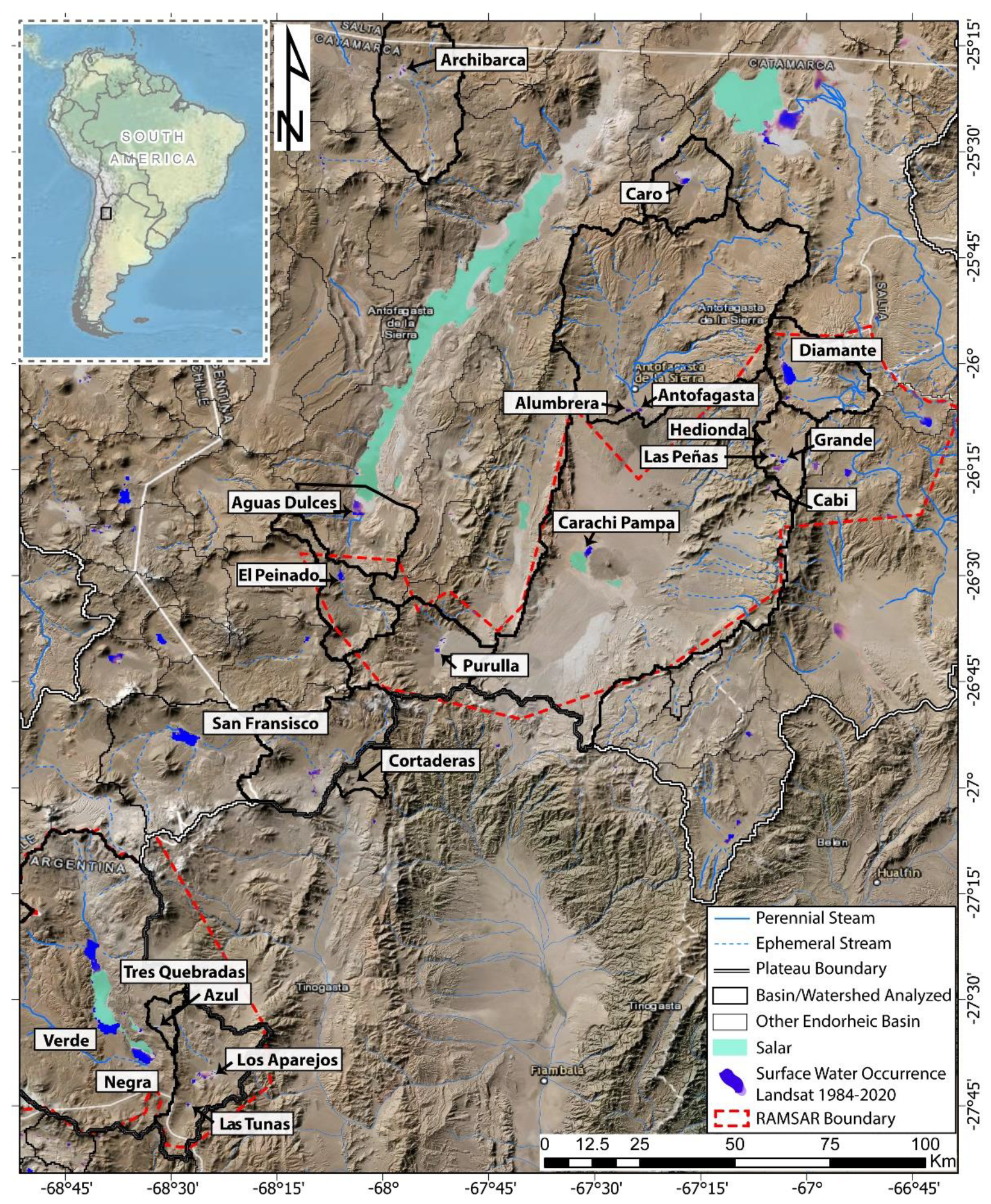
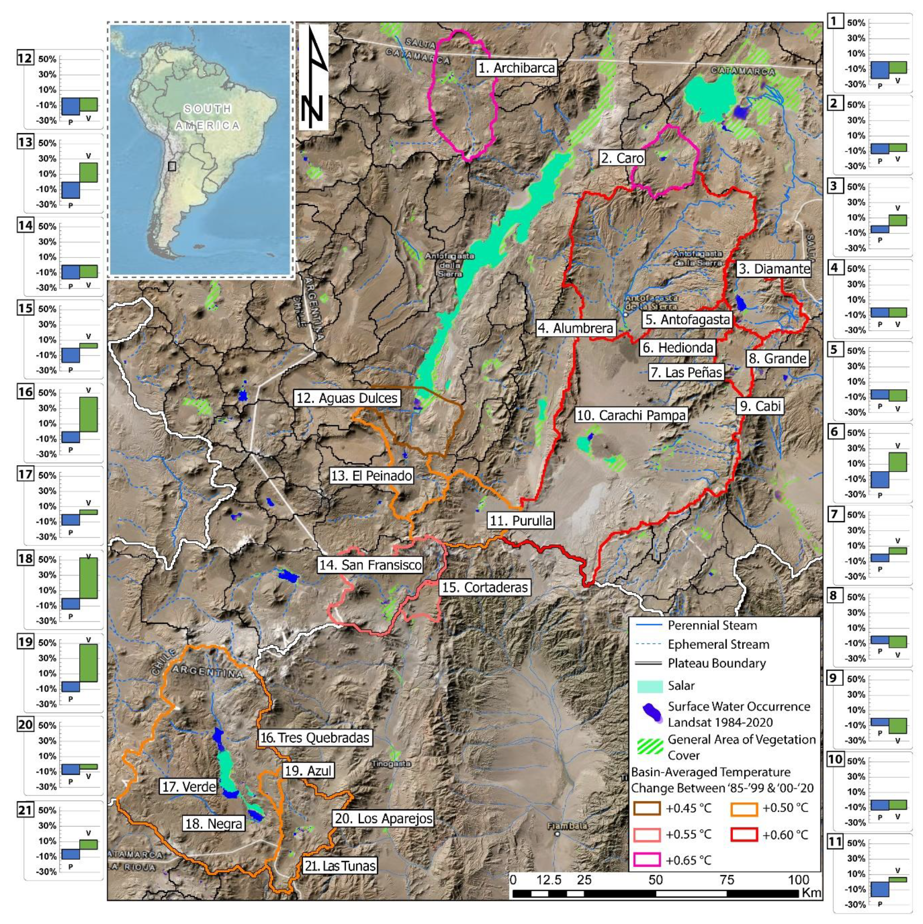
2.1. Study Area
2.2. Physical-Chemical Sampling and Laboratory Analyses
2.3. Hydroclimate Characterization
2.4. Biological Sampling and Analyses
3. Results
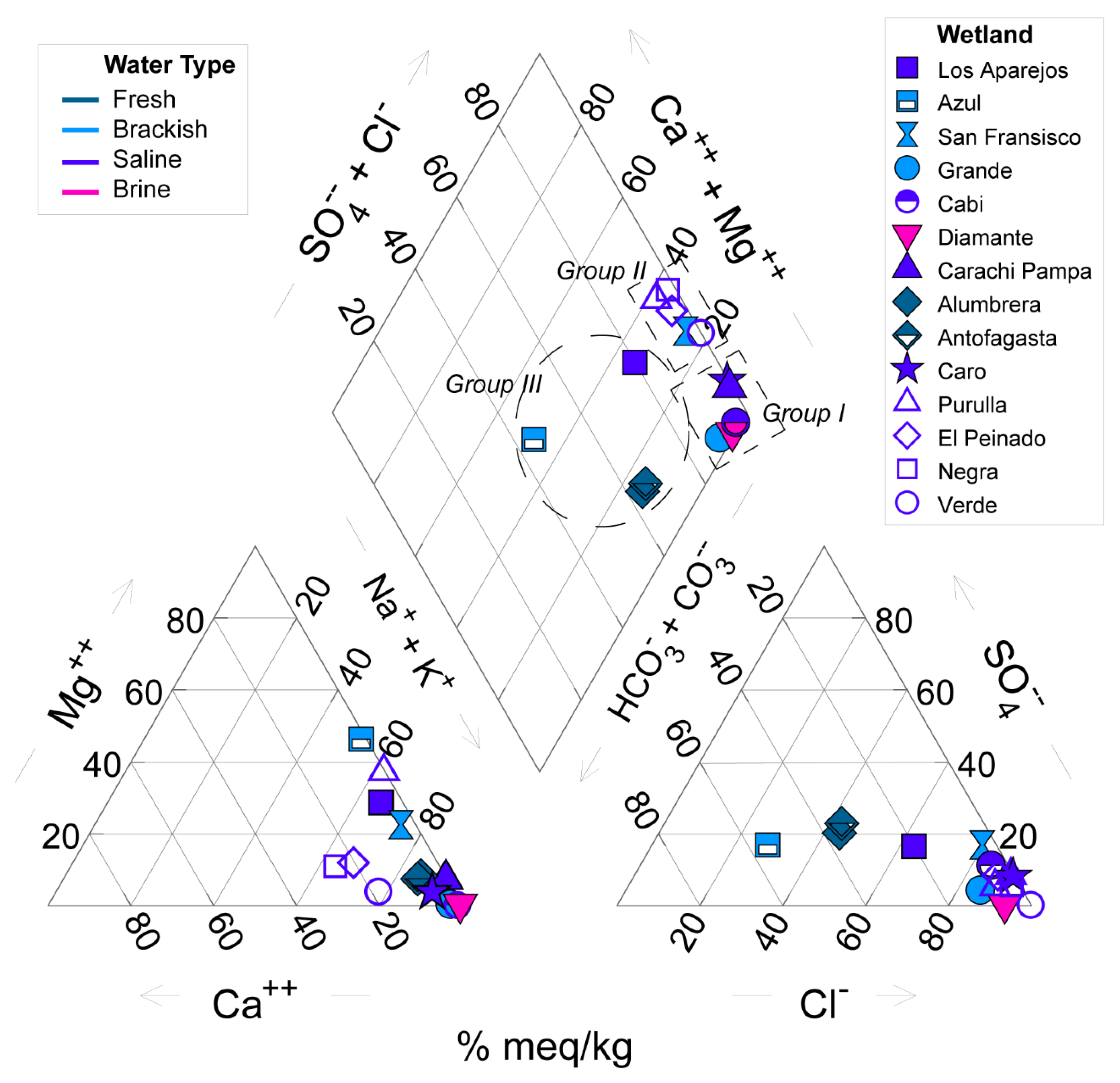
3.1. Physical-Chemical and Hydroclimate Characterization
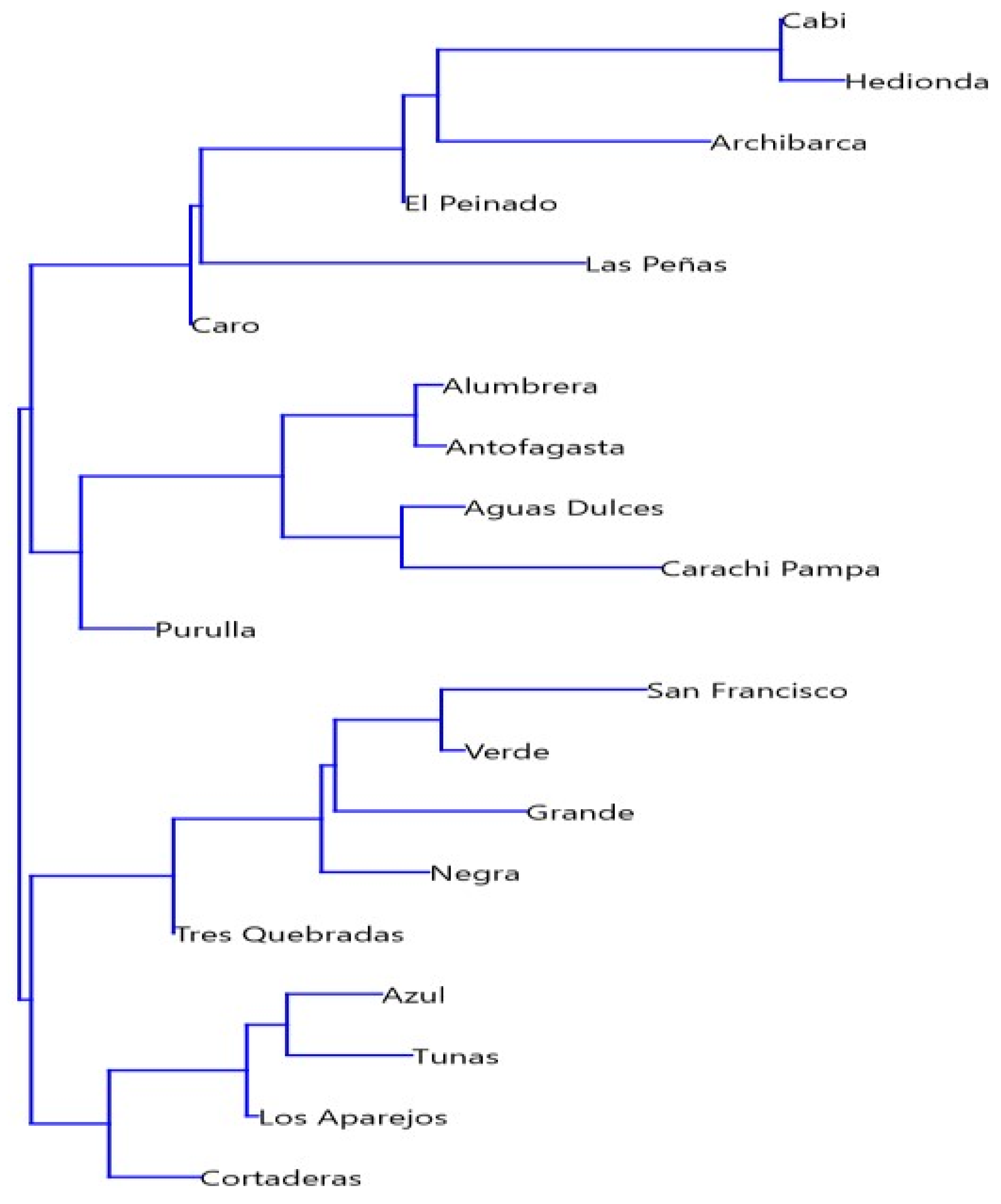
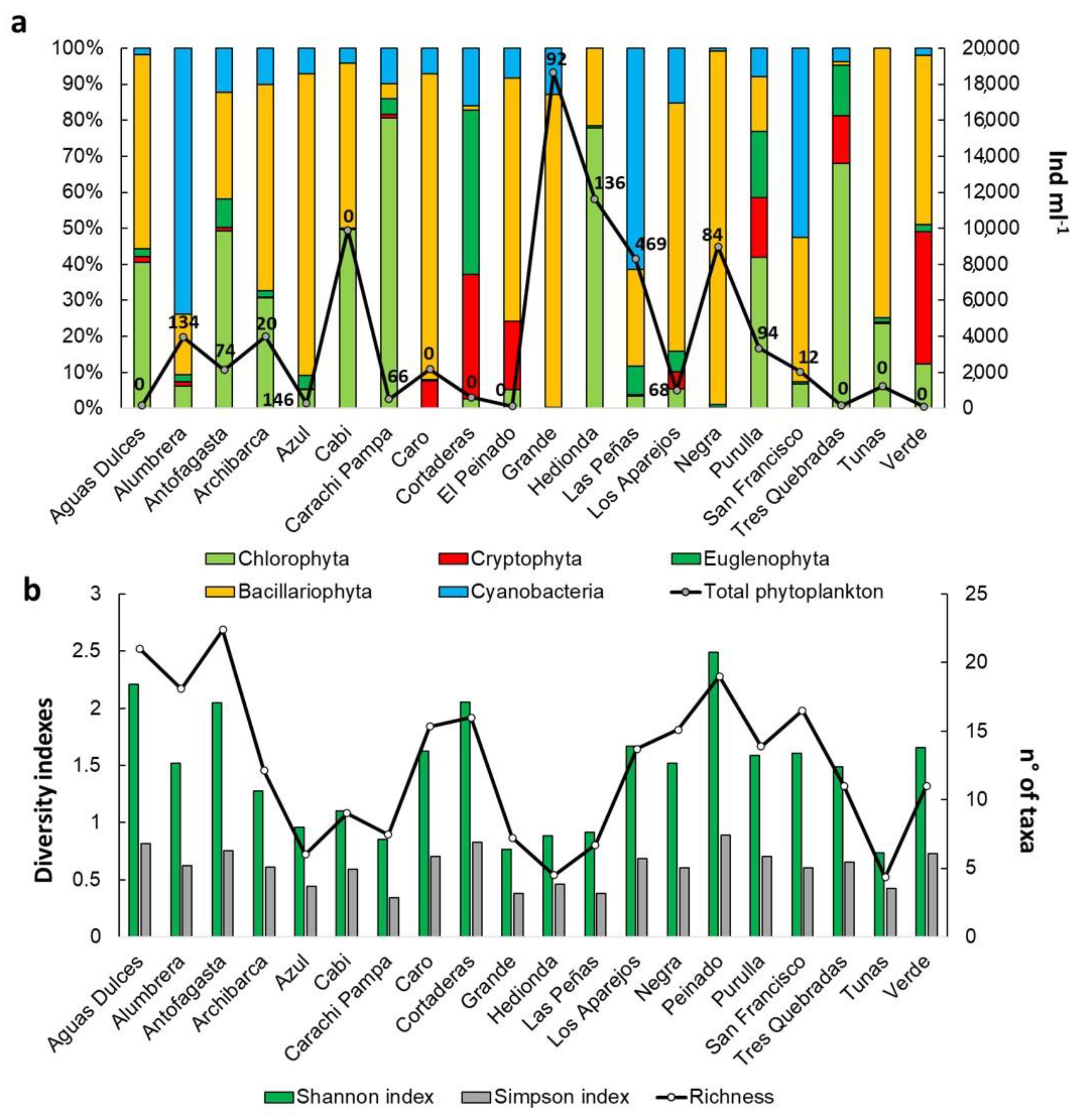
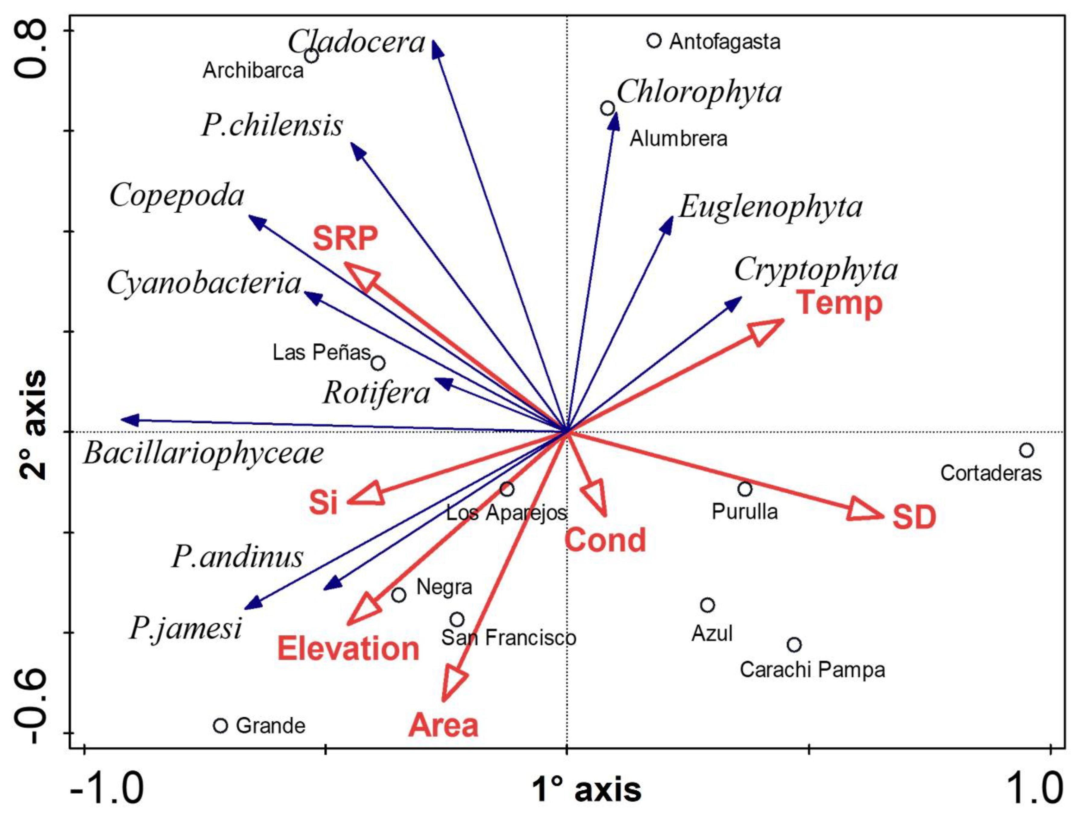
3.2. Biological Communities’ Characterization
4. Discussion
4.1. Geological, Hydrological, and Climatological Features
4.2. Biological Communities’ Characterization
5. Conclusions
Supplementary Materials
Author Contributions
Funding
Acknowledgments
Conflicts of Interest
References
- Allmendinger, R.W.; Jordan, T.E.; Kay, S.M.; Isacks, B.L. The evolution of the Altiplano-Puna plateau of the Central Andes. Annu. Rev. Earth Planet. Sci. 1997, 25, 139–174. [Google Scholar] [CrossRef]
- Jordan, T.E.; Nester, P.L.; Blanco, N.; Hoke, G.D.; Dávila, F.; TomLinson, A.J. Uplift of the Altiplano-Puna plateau: A view from the west. Tectonics 2010, 29, TC5007. [Google Scholar] [CrossRef]
- Álvarez Blanco, I.; Cejudo-Figueiras, C.; de Godos, I.; Muñoz, R.; Blanco, S. Las diatomeas de los salares del Altiplano boliviano: Singularidades florísticas. Boletín Real Soc. Española Hist. Nat. Sección Biológica 2011, 105, 67–82. [Google Scholar]
- Scott, S.; Dorador, C.; Yanedel, J.P.; Tobar, I.; Hengst, M.; Maya, G.; Harrod, C.; Vila, I. Microbial diversity and trophic components of two high elevation wetlands of the Chilean Altiplano. Gayana 2015, 79, 45–56. [Google Scholar] [CrossRef] [Green Version]
- Williams, W.D.; Boulton, A.J.; Taaffe, R.G. Salinity as a determinant of salt lake fauna: A question of scale. Hydrobiologia 1990, 197, 257–266. [Google Scholar] [CrossRef]
- De la Fuente, A.; Meruane, C.; Suárez, F. Long-term spatiotemporal variability in high Andean wetlands in northern Chile. Sci. Total Environ. 2021, 756, 143830. [Google Scholar] [CrossRef]
- Eugster, H.P. Geochemistry of evaporitic lacustrine deposits. Annu. Rev. Earth Planet. Sci. 1980, 8, 35–63. [Google Scholar] [CrossRef]
- Risacher, F.; Alonso, H.; Salazar, C. The origin of brines and salts in Chilean salars: A hydrochemical review. Earth-Sci. Rev. 2003, 63, 249–293. [Google Scholar] [CrossRef]
- Psenner, R. Alpine waters in the interplay of global change: Complex links-simple effects? In Global Environmental Change in the Alpine Region. New Horizons in Environmental Economics; Steininger, K.W., Weck-Hannemann, H., Eds.; Edward Eldgar: Gloucestershire, UK, 2002. [Google Scholar]
- Boyle, T.P.; Caziani, S.M.; Waltermire, R.G. Landsat TM inventory and assessment of waterbird habitat in the southern altiplano of South America. Wetl. Ecol. Manag. 2004, 12, 563–573. [Google Scholar] [CrossRef]
- Squeo, F.A.; Warner, B.G.; Aravena, R.; Espinoza, D. Bofedales: High elevatione peatlands of the central Andes. Rev. Chil. Hist. Nat. 2006, 79, 245–255. [Google Scholar] [CrossRef] [Green Version]
- Valois, R.; Schaer, N.; Figueroa, R.; Maldonado, A.; Yáñez, E.; Hevia, A.; Yánez Carrizo, G.; MacDonell, S. Characterizing the Water Storage Capacity and Hydrological Role of Mountain Peatlands in the Arid Andes of North-Central Chile. Water 2020, 12, 1071. [Google Scholar] [CrossRef] [Green Version]
- Gleeson, T.; Marklund, L.; Smith, L.; Manning, A.H. Classifying the water table at regional to continental scales. Geophys. Res. Lett. 2011, 38, L05401. [Google Scholar] [CrossRef]
- Walvoord, M.A.; Plummer, M.A.; Phillips, F.M.; Wolfsberg, A.V. Deep arid system hydrodynamics: 1. Equilibrium states and response times in thick desert vadose zones. Water Resour. Res. 2002, 38, 1308. [Google Scholar] [CrossRef] [Green Version]
- Liu, Y.; Wagener, T.; Beck, H.E.; Hartmann, A. What is the hydrologically effective area of a catchment? Environ. Res. Lett. 2020, 15, 104024. [Google Scholar] [CrossRef]
- Boutt, D.F.; Corenthal, L.G.; Moran, B.J.; Munk, L.A.; Hynek, S.A. Imbalance in the modern hydrologic budget of topographic catchments along the western slope of the Andes (21–25°S): Implications for groundwater recharge assessment. Hydrogeol. J. 2021, 29, 985–1007. [Google Scholar] [CrossRef]
- Alley, W.M.; Healy, R.W.; LaBaugh, J.W.; Reilly, T.E. Flow and storage in groundwater systems. Science 2002, 296, 1985–1990. [Google Scholar] [CrossRef] [Green Version]
- Maxwell, R.M.; Condon, L.E.; Kollet, S.J.; Maher, K.; Haggerty, R.; Forrester, M.M. The imprint of climate and geology on the residence times of groundwater. Geophys. Res. Lett. 2016, 43, 701–708. [Google Scholar] [CrossRef] [Green Version]
- Corenthal, L.G.; Boutt, D.F.; Hynek, S.A.; Munk, L.A. Regional groundwater flow and accumulation of a massive evaporite deposit at the margin of the Chilean Altiplano. Geophys. Res. Lett. 2016, 43, 8017–8025. [Google Scholar] [CrossRef]
- Munk, L.A.; Boutt, D.F.; Hynek, S.A.; Moran, B.J. Hydrogeochemical fluxes and processes contributing to the formation of lithium-enriched brines in a hyper-arid continental basin. Chem. Geol. 2018, 493, 37–57. [Google Scholar] [CrossRef]
- Moran, B.J.; Boutt, D.F.; Munk, L.A. Stable and Radioisotope Systematics Reveal Fossil Water as Fundamental Characteristic of Arid Orogenic-Scale Groundwater Systems. Water Resour. Res. 2019, 55, 11295–11315. [Google Scholar] [CrossRef] [Green Version]
- Munk, L.A.; Boutt, D.F.; Moran, B.J.; McKnight, S.V.; Jenckes, J. Hydrogeologic and Geochemical Distinctions in Freshwater-Brine Systems of an Andean Salar. Geochem. Geophys. 2021, 22, e2020GC009345. [Google Scholar]
- Izquierdo, A.E.; Aragón, R.; Navarro, C.J.; Casagranda, E. Humedales de la Puna: Principales proveedores de servicios ecosistémicos de la región. In Serie de Conservación de la Naturaleza 24: La Puna Argentina: Naturaleza y Cultura; Grau, H.R., Babot, M.J., Izquierdo, A., Grau, A., Eds.; Fundación Miguel Lillo: Tucumán, Argentina, 2018; pp. 96–111. [Google Scholar]
- Gluzman, G. Minería y metalurgia en la antigua gobernación del Tucumán (siglos XVI–XVII): Colonial Tucumán 16th and 17th Centuries. Mem. Am. 2007, 15, 157–184. [Google Scholar]
- Kesler, S.E.; Gruber, P.W.; Medina, P.A.; Keoleian, G.A.; Everson, M.P.; Wallington, T.J. Global lithium resources: Relative importance of pegmatite, brine and other deposits. Ore Geol. Rev. 2012, 48, 55–69. [Google Scholar] [CrossRef]
- Munk, L.A.; Hynek, S.A.; Bradley, D.; Boutt, D.F.; Labay, K.; Jochens, H. Lithium brines: A global perspective. Rev. Econ. Geol. 2016, 18, 339–365. [Google Scholar]
- Williams, W.D. Environmental threats to salt lakes and the likely status of inland saline ecosystems in 2025. Environ. Conserv. 2002, 29, 154–167. [Google Scholar] [CrossRef] [Green Version]
- Tolotti, M.; Thies, M.; Cantonati, M.; Hansen, C.; Thaler, B. Flagellate algae (Chrysophyceae, Dinophyceae, Cryptophyceae) in 48 high mountain lakes of the Northern and Southern slope of the Eastern Alps: Biodiversity, taxa distribution and their driving variables. Hydrobiologia 2006, 502, 331–348. [Google Scholar] [CrossRef]
- Meehl, G.A.; Arblaster, J.M.; Tebaldi, C. Understanding future patterns of increased precipitation intensity in climate model simulations. Geophys. Res. Lett. 2005, 32, L18719. [Google Scholar] [CrossRef] [Green Version]
- Urrutia, R.; Vuille, M. Climate change projections for the tropical Andes using a regional climate model: Temperature and precipitation simulations for the end of the 21st century. J. Geophys. Res. 2009, 114, D02108. [Google Scholar] [CrossRef]
- Barros, V.R.; Boninsegna, J.A.; Camilloni, I.A.; Chidiak, M.; Magrín, G.O.; Rusticucci, M. Climate change in Argentina: Trends, projections, impacts and adaptation. Wiley Interdiscip. Rev. Clim. Chang. 2015, 6, 151–169. [Google Scholar] [CrossRef]
- Pabón-Caicedo, J.D.; Arias, P.A.; Carril, A.F.; Espinoza, J.C.; Borrel, L.F.; Goubanova, K.; Lavado-Casimiro, W.; Masiokas, M.; Solman, S.; Villalba, R. Observed and Projected Hydroclimate Changes in the Andes. Front. Earth Sci. 2020, 8, 61. [Google Scholar] [CrossRef]
- Ibarguchi, G. From Southern Cone arid lands, across Atacama, to the Altiplano: Biodiversity and conservation at the ends of the world. Biodiversity 2014, 15, 255–264. [Google Scholar] [CrossRef]
- Aguilar, P.; Dorador, C.; Vila, I.; Sommaruga, R. Bacterioplankton composition in tropical high-elevation lakes of the Andean plateau. FEMS Microbiol. Ecol. 2018, 94, fiy004. [Google Scholar] [CrossRef] [Green Version]
- Farías, E. Microbial Ecosystems in Central Andes Extreme Environments; Springer International Publishing: Cham, Switzerland, 2020. [Google Scholar]
- Locascio de Mitrovic, C.A.; Villagra de Gamundi, A.; Juárez, J.; Ceraolo, M. Características limnológicas y zooplancton de cinco lagunas de la Puna-Argentina. Ecol. Boliv. 2005, 40, 12–26. [Google Scholar]
- Aguilera, X.; Declercka, S.; De Meester, L.; Maldonado, M.; Ollevier, F. Tropical high Andes lakes: A limnological survey and an assessment of exotic rainbow trout (Oncorhynchus mykiss). Limnologica 2006, 36, 258–268. [Google Scholar] [CrossRef] [Green Version]
- Seeligmann, C.; Maidana, N.I.; Morales, M. Diatomeas (Bacillariophyceae) de humedales de altura de la provincia de Jujuy-Argentina. Boletín Soc. Argent. Botánica 2008, 43, 1–17. [Google Scholar]
- Maidana, N.I.; Seeligmann, C.T.; Morales, M.R. Bacillariophyceae del Complejo Lagunar Vilama (Jujuy, Argentina). Boletín Soc. Argent. Botánica 2009, 44, 257–271. [Google Scholar]
- Mirande, V.; Tracanna, B. Estructura y controles abióticos del fitoplancton en humedales de altura. Ecol. Austral 2009, 19, 119–128. [Google Scholar]
- Declerck, S.A.J.; Coronel, J.S.; Legendre, P.; Brendonck, L. Scale dependency of processes structuring metacommunities of cladocerans in temporary pools of High-Andes wetlands. Ecography 2011, 34, 296–305. [Google Scholar] [CrossRef] [Green Version]
- Caputo, L.; Giuseppe, A.; Givovich, A. Limnological features of Laguna Teno (35° S, Chile): A high-elevation lake impacted by volcanic activity. Fundam. Appl. Limnol. 2013, 183, 323–335. [Google Scholar] [CrossRef]
- Albarracín, V.H.; Kurth, D.; Ordoñez, O.F.; Belfiore, C.; Luccini, E.; Salum, G.M.; Piacentini, R.D.; Farías, M.E. High-Up: A Remote Reservoir of Microbial Extremophiles in Central Andean Wetlands. Front. Microbiol. 2015, 6, 1404. [Google Scholar] [CrossRef] [Green Version]
- Servant-Vildary, S.; Roux, M. Multivariate analysis of diatoms and water chemistry in Bolivian saline lakes. In Saline Lakes Developments in Hydrobiology; Comínand, F., Northcote, T., Eds.; Springer: Leiden, The Netherlands, 1990; pp. 267–290. [Google Scholar]
- Rejas, D.; Valverde, C.; Fernández, C.E. Limitación por nutrientes y pastoreo como factores de control de las densidades de bacterias y algas planctónicas en una laguna altoandina (Cochabamba, Bolivia). Rev. Boliv. Ecol. Conserv. Ambient. 2012, 30, 1–12. [Google Scholar]
- Frau, D.; Battauz, Y.; Mayora, G.; Marconi, P. Controlling factors in planktonic communities over a salinity gradient in high-elevation lakes. Ann. Limnol.-Int. J. Limnol. 2015, 51, 261–272. [Google Scholar]
- Fjeldså, J.; Krabbe, N.K. Birds of the High Andes; Museum Tusculanum Press: Copenhagen, Denmark, 1990; 881p. [Google Scholar]
- Caziani, S.M.; Derlindati, E.J.; Tálamo, A.; Sureda, A.L.; Trucco, C.E.; Nicolossi, G. Waterbird richness in altiplano wetlands of northwestern Argentina. Waterbirds 2001, 24, 103–117. [Google Scholar] [CrossRef]
- Vuilleumier, F.; Simberloff, D. Ecology versus history as determinants of patchy and insular distribution in high Andean birds. In Evolutionary Biology; Hecht, M., Steere, W., Wallace, B., Eds.; Plenum Publishing Corporation: New York, NY, USA, 1980; pp. 235–379. [Google Scholar]
- Tellería, J.L.; Venero, J.L.; Santos, T. Conserving birdlife of Peruvian highland bogs: Effects of patch-size and habitat quality on species richness and bird numbers. Ardeola 2006, 53, 271–283. [Google Scholar]
- Jacobsen, D.; Dangles, O. Ecology of High. Elevation Waters; Oxford University Press: Oxford, MS, USA, 2017. [Google Scholar]
- Castellino, M.; Lesterhuis, A. Censo Simultáneo de Falaropos 2020-Resumen y Resultados; Manomet-WHSRN: Plymouth, MA, USA, 2020. [Google Scholar]
- Caziani, S.M.; Rocha, O.; Rodríguez Ramírez, E.; Romano, M.C.; Derlindati, E.J.; Tálamo, A.; Ricalde, D.; Quiroga, C.; Contreras, J.P.; Valqui, M.; et al. Seasonal distribution, abundance, and nesting of Puna, Andean, and Chilean flamingos. Condor 2007, 109, 276–287. [Google Scholar] [CrossRef]
- Marconi, P.; Sureda, A.L.; Arengo, F.; Aguilar, M.S.; Amado, N.; Alza, L.; Rocha, O.; Torres, R.; Moschione, F.; Romano, M.; et al. Fourth simultaneous flamingo census in South America: Preliminary results. Flamingo 2011, 18, 48–53. [Google Scholar]
- Marconi, P.; Arengo, F.; Castro, A.; Rocha, O.; Valqui, M.; Aguilar, S.; Barberis, I.; Castellino, M.; Castro, L.; Derlindati, E.; et al. Sixth International Simultaneous Census of three flamingo species in the Southern Cone of South America: Preliminary Analysis. Flamingo 2020, 12, 67–75. [Google Scholar]
- Villagrán, C.; Castro, V. Ciencia Indígena de Los Andes del Norte de Chile; Editorial Universitaria: Santiago, Chile, 1997; p. 362. [Google Scholar]
- Catalan, J.; Rondón, J.C.D. Perspectives for an integrated understanding of tropical and temperate high-mountain lakes. J. Limnol. 2016, 75, 215–234. [Google Scholar] [CrossRef] [Green Version]
- Adrian, R.; O’Reilly, C.M.; Zagarese, H.; Baines, S.B.; Hessen, D.O.; Keller, W.; Livingstone, D.M.; Sommaruga, R.; Straile, D.; Van Donk, E.; et al. Lakes as sentinels of climate change. Limnol. Oceanogr. 2009, 54, 2283–2297. [Google Scholar] [CrossRef]
- Coronel, J.S.; Declerck, S.; Maldonado, M.; Ollevier, F.; Brendonck, L. Temporary shallow pools in the high-Andes ‘bofedal’ peat lands: A limnological characterization at different spatial scales. Arch. Sci. 2004, 57, 85–96. [Google Scholar]
- Wanger, T.C. The Lithium future—Resources, recycling, and the environment. Conserv. Lett. 2011, 4, 202–206. [Google Scholar] [CrossRef]
- Marconi, P.; Arengo, F.; Clark, A. The arid Andean plateau waterscapes and the lithium triangle: Flamingos as flagships for conservation of wetlands under pressure from mining development. Wetl. Ecol. Manag. 2021. under review. [Google Scholar]
- Morlans, M.C. Regiones Naturales de Catamarca. Provincias Geológicas y Provincias Fitogeográficas. Rev. Cienc. Técnica 1995, 2, 1–42. [Google Scholar]
- Pekel, J.F.; Cottam, A.; Gorelick, N.; Belward, A.S. High-resolution mapping of global surface water and its long-term changes. Nature 2016, 540, 418–422. [Google Scholar] [CrossRef]
- Warren, J.K. Evaporites: A Geological Compendium; Springer International Publishing: Cham, Switzerland, 2016; p. 1813. [Google Scholar]
- Hilton, J.; Rigg, E. Determination of nitrate in lake water by the adaptation of the hydrazine-copper reduction method for use on a discrete analyser: Performance statistics and an instrument-induced difference from segmented flow conditions. Analyst 1993, 108, 1026–1028. [Google Scholar] [CrossRef]
- APHA. Standard Methods for the Examination of Water and Wastewater; American Public Health Association: Washington, DC, USA, 2005. [Google Scholar]
- Sureda, A.L. Patrones de Diversidad en Aves de Lagunas Altoandinas de Catamarca, Noroeste de Argentina. Licentiate Thesis, Universidad Nacional de Salta, Salta, Argentina, 2003; p. 63. [Google Scholar]
- Lehner, B.; Grill, G. Global River hydrography and network routing: Baseline data and new approaches to study the world’s large river systems. Hydrol. Process. 2013, 27, 2171–2186. [Google Scholar] [CrossRef]
- Abatzoglou, J.T.; Dobrowski, S.Z.; Parks, S.A.; Hegewisch, K.C. TerraClimate, a high-resolution global dataset of monthly climate and climatic water balance from 1958–2015. Sci. Data 2018, 5, 170191. [Google Scholar] [CrossRef] [Green Version]
- McNally, A.; Arsenault, K.; Kumar, S.; Shukla, S.; Peterson, P.; Wang, S.; Funk, C.; Peters-Lidard, C.D.; Verdin, J.P. A land data assimilation system for sub-Saharan Africa food and water security applications. Sci. Data 2017, 4, 170012. [Google Scholar] [CrossRef] [Green Version]
- Tucker, C.J. Red and photographic infrared linear combinations for monitoring vegetation. Remote Sens. Environ. 1979, 8, 127–150. [Google Scholar] [CrossRef] [Green Version]
- Utermöhl, H. Zur Vervollkommnung der quantitativen Phytoplankton. Methodik. Mitt. Int. Verein. Limnol. 1958, 9, 1–38. [Google Scholar]
- Venrick, E.L. How many cells to count? In Phytoplankton Manual; Von Sournia, A., Ed.; UNSECO: Paris, France, 1978; pp. 167–180. [Google Scholar]
- Lee, R.D. Phycology; Cambridge University Press: Cambridge, UK, 2008. [Google Scholar]
- Krammer, K.; Lange-Bertalot, H. Bacillariophyceae. 3. Teil Centrales, Fragilariaceae, Eunotiaceae. In Süsswasserflora von Mitteleuropa; Ettl, H., Gerloff, J., Heynig, H., Mollenhauer, D., Eds.; Gustav Fischer Verlag: Stuttgar, Germany, 1991. [Google Scholar]
- Tell, G.; Conforti, V. Euglenophyta pigmentadas da Argentina. Bibl. Phycol. 1986, 75, 1–301. [Google Scholar]
- Komárek, J.; Fott, B. Chlorophyceae, chlorococcales. In Das Phytoplankton des Sdwasswes. Die Binnenggewasser; Huber-Pestalozzi, G., Ed.; Schweizerbart’sche Verlagsbuchhandlung: Stuttgart, Germany, 1983. [Google Scholar]
- Komárek, J.; Anagnostidis, K. Cyanoprokariota. 1. Chroococcales. In Subwasserflora von Mitteleuropa; Ett, H., Gärdner, G., Heynig, H., Mollenhauer, D., Eds.; Gustav Fischer Verlag: Stuttgar, Germany, 1999. [Google Scholar]
- Komárek, J.; Anagnostidis, K. Cyanoprokaryota. Teil 2: Oscillatoriales. In Süsswasserflora von Mitteleuropa 19/2; Büdel, B., Gärtner, G., Krienitz, L., Schagerl, M., Eds.; Elsevier: München, Germany, 2005. [Google Scholar]
- Ahlstrom, E.H. A revision of the Rotatorian genera Brachionus and Platyias with descriptions of one new species and two new varieties. Bull. Am. Mus. Nat. Hist. 1940, 77, 143–148. [Google Scholar]
- Koste, W. Rotatoria. Die Radertiere Mitteleuropas; Gebruder Borntraeger: Berlin, Germany, 1978. [Google Scholar]
- Kořínek, V. Diaphanosoma birgei n.sp. (Crustacea, Cladocera). A new species from America and its widely distributed subspecies Diaphanosoma birgei ssp. lacustris n.ssp. Can. J. Zool. 1981, 59, 1115–1121. [Google Scholar] [CrossRef]
- Kořínek, V. Cladocera. In A Guide to Tropical Freshwater Zooplankton; Fernando, C.H., Ed.; Backhuys Publishers: Leiden, The Netherlands, 2002; pp. 69–122. [Google Scholar]
- Korovchinski, N.M. Sididae and Holopedidae (Crustacea: Daphniiformes). In Guides to Identification of the Microinvertebrates of the Continental Waters of the World; SPB Academic Publishers: The Hague, The Netherlands, 1992. [Google Scholar]
- Alekseev, V.R. Copepoda. In A Guide to Tropical. Freshwater Zooplankton; Fernando, C.H., Ed.; Backhugs Publishers: Leiden, The Netherlands, 2002; pp. 123–188. [Google Scholar]
- Marconi, P. Técnicas de monitoreo de condiciones ecológicas en la Red de Humedales de Importancia para la Conservación de Flamencos Altoandinos. In Manual de Técnicas de Monitoreo de Condiciones Ecológicas para el Manejo Integrado de la red de Humedales de Importancia para la Conservación de Flamencos Altoandinos; Marconi, P., Ed.; Fundación YUCHAN: Salta, Argentina, 2010; pp. 8–14. [Google Scholar]
- Messager, M.L.; Lehner, B.; Grill, G.; Nedeva, I.; Schmitt, O. Estimating the volume and age of water stored in global lakes using a geo-statistical approach. Nat. Commun. 2016, 7, 13603. [Google Scholar] [CrossRef] [PubMed]
- Pingel, H.; Alonso, R.N.; Altenberger, U.; Cottle, J.; Strecker, M.R. Miocene to Quaternary basin evolution at the southeastern Andean Plateau (Puna) margin (ca. 24°S lat, Northwestern Argentina). Basin Res. 2019, 31, 808–826. [Google Scholar] [CrossRef]
- Gamboa, C.; Godfrey, L.; Herrera, C.; Custodio, E.; Soler, A. The origin of solutes in groundwater in a hyper-arid environment: A chemical and multi-isotope approach in the Atacama Desert, Chile. Sci. Total Environ. 2019, 690, 329–351. [Google Scholar] [CrossRef]
- Reynolds, C.S. The Ecology of Phytoplankton; Cambridge University Press: Cambridge, UK, 2006; p. 552. [Google Scholar]
- Cloern, J.E.; Alpine, A.E.; Cole, B.E.; Wong, R.L.J.; Arthur, J.F.; Ball, M.D. River discharge controls phytoplankton dynamics in the northern San Francisco Bay estuary. Estuar. Coast. Shelf Sci. 1983, 16, 415–429. [Google Scholar] [CrossRef]
- Herbst, D.B.; Bradley, T.J. A Malpighian tubule lime gland in an insect inhabiting alkaline salt lakes. J. Exp. Biol. 1989, 145, 63–78. [Google Scholar] [CrossRef]
- Salm, C.R.; Saros, J.E.; Martin, C.S.; Erickson, J.M. Patterns of seasonal phytoplankton distribution in prairie saline lakes of the northern Great Plains (U.S.A.). Saline Syst. 2009, 5, 1. [Google Scholar] [CrossRef] [PubMed] [Green Version]
- Salm, C.R.; Saros, J.E.; Fritz, S.C.; Osburn, C.L.; Reineke, D.M. Phytoplankton productivity across prairie saline lakes of the Great Plains (USA): A step toward deciphering patterns through lake classification models. Can. J. Fish. Aquat. Sci. 2009, 66, 1435–1448. [Google Scholar] [CrossRef] [Green Version]
- Sánchez Carrillo, S.; Álvarez-Cobelas, M. Nutrient Dynamics and Eutrophication Patterns in A Semi-Arid Wetland: The Effects of Fluctuating Hydrology. Water Air Soil Pollut. 2001, 131, 97–118. [Google Scholar] [CrossRef]
- Sánchez Carrillo, S.; Angeler, D.G.; Alvarez-Cabelas, M.; Sanchez-Andres, R. Freshwater wetland eutrophication. In Eutrophication: Causes, Consequences and Control; Ansari, A.A., Singh Gill, S., Lanza, G.R., Rast, W., Eds.; Springer: Heidelberg, Germany, 2011; pp. 195–210. [Google Scholar]
- Jordan, T.E.; Mpodozis, C.; Muñoz, N.; Blanco, N.; Pananont, P.; Gardeweg, M. Cenozoic subsurface stratigraphy and structure of the Salar de Atacama Basin, northern Chile. J. S. Am. Earth Sci. 2007, 23, 122–146. [Google Scholar] [CrossRef]
- Salisbury, M.J.; Jicha, B.R.; de Silva, S.L.; Singer, B.S.; Jiménez, N.C.; Ort, M.H. 40Ar/39Ar chronostratigraphy of Altiplano-Puna volcanic complex ignimbrites reveals the development of a major magmatic province. Geol. Soc. Am. Bull. 2011, 123, 821–840. [Google Scholar] [CrossRef]
- Finstad, K.; Pfeiffer, M.; McNicol, G.; Barnes, J.; Demergasso, C.; Chong, G.; Amundson, R. Rates and geochemical processes of soil and salt crust formation in Salars of the Atacama Desert, Chile. Geoderma 2016, 284, 57–72. [Google Scholar] [CrossRef]
- Leopold, L.B. Temperature profiles and bathymetry of some high mountain lakes. Proc. Natl. Acad. Sci. USA 2000, 97, 6267–6270. [Google Scholar] [CrossRef] [PubMed] [Green Version]
- Muñoz, R.; Huggel, C.; Frey, H.; Cochachin, A.; Haeberli, W. Glacial Lake depth and volume estimation based on a large bathymetric dataset from the Cordillera Blanca, Peru. Earth Surf. Process. Landf. 2020, 45, 1510–1527. [Google Scholar] [CrossRef]
- Boutt, D.F.; Hynek, S.A.; Munk, L.A.; Corenthal, L.G. Rapid recharge of fresh water to the halite-hosted brine aquifer of Salar de Atacama, Chile. Hydrol. Process. 2016, 30, 4720–4740. [Google Scholar] [CrossRef]
- Price, J.S. Hydrology and microclimate of a partly restored cutover bog, Quebec. Hydrol. Process. 1996, 10, 1263–1272. [Google Scholar] [CrossRef]
- Plach, J.M.; Petrone, R.M.; Waddington, J.M.; Kettridge, N.; Devito, K.J. Hydroclimatic influences on peatland CO2 exchange following upland forest harvesting on the Boreal Plains. Ecohydrology 2016, 9, 1590–1603. [Google Scholar] [CrossRef] [Green Version]
- Jordan, T.E.; Herrera, L.C.; Godfrey, L.V.; Colucci, S.J.; Gamboa, P.C.; Urrutia, M.J.; González, G.L.; Paul, J.F. Isotopic characteristics and paleoclimate implications of the extreme precipitation event of March 2015 in Northern Chile. Andean Geol. 2019, 46, 1–31. [Google Scholar] [CrossRef]
- Langenbrunner, B.; Pritchard, M.S.; Kooperman, G.J.; Randerson, J.T. Why does Amazon precipitation decrease when tropical forests respond to increasing CO2? Earth’s Future 2019, 7, 450–468. [Google Scholar] [CrossRef] [Green Version]
- Pascale, S.; Carvalho, L.M.V.; Adams, D.K.; Castro, C.L.; Cavalcanti, I.F.A. Current and future variations of the monsoons of the Americas in a warming climate. Curr. Clim. Chang. Rep. 2019, 5, 125–144. [Google Scholar] [CrossRef]
- Garreaud, R.D.; Boisier, J.P.; Rondanelli, R.; Montecinos, A.; Sepúlveda, H.H.; Veloso-Aguila, D. The Central Chile Mega Drought (2010–2018): A climate dynamics perspective. Int. J. Climatol. 2020, 40, 421–439. [Google Scholar] [CrossRef]
- Ferrero, M.E.; Villalba, R. Interannual and long-term precipitation variability along the subtropical mountains and adjacent Chaco (22–29° S) in Argentina. Front. Earth Sci. 2019, 7, 148. [Google Scholar] [CrossRef] [Green Version]
- Petrone, R.M.; Devito, K.J.; Silins, U.; Mendoza, C.; Brown, S.C.; Kaufman, S.C.; Price, J.S. Transient peat properties in two pond-peatland complexes in the sub-humid Western Boreal Plain, Canada. Mires Peat 2008, 3, 1–13. [Google Scholar]
- Rolando, J.L.; Turina, C.; Ramírez, D.A.; Maresa, V.; Monerris, J.; Quiroz, R. Key ecosystem services and ecological intensification of agriculture in the tropical high-Andean Puna as affected by land-use and climate changes. Agric. Ecosyst. Environ. 2017, 236, 221–233. [Google Scholar] [CrossRef]
- Moran, B.J.; Boutt, D.F.; McKnight, S.V.; Jenckes, J.; Munk, L.A.; Corkran, D.; Kirshen, A. Water Sustainability, Drought, Relic Groundwater and Lithium Resource Extraction in an Arid Landscape; University of Massachusetts: Amherst, MA, USA, 2021; Manuscript to be submitted. [Google Scholar]
- García, A.; Ulloa, C.; Amigo, G.; Milana, J.P.; Medina, C. An inventory of cryospheric landforms in the arid diagonal of South America (high Central Andes, Atacama region, Chile). Quat. Int. 2017, 438, 4–19. [Google Scholar] [CrossRef]
- Schaffer, N.; MacDonell, S.; Réveillet, M.; Yáñez, E.; Valois, R. Rock glaciers as a water resource in a changing climate in the semiarid Chilean Andes. Reg. Environ. Chang. 2019, 19, 1263–1279. [Google Scholar] [CrossRef]
- Moran, B.J.; Boutt, D.F.; Munk, L.A.; Fisher, J.D. Pronounced Water Age Partitioning Between Arid Andean Aquifers and Fresh-Saline Lagoon Systems. In Proceedings of the EGU General Assembly 2021a, online/virtual, 19–30 April 2021. EGU21-13753. [Google Scholar] [CrossRef]
- Canevari, P. El Flamenco Común; Centro Editor de América Latina: Buenos Aires, Argentina, 1983. [Google Scholar]
- Bucher, E.H. Flamencos. In Bañados del río Dulce y Laguna Mar Chiquita; Bucher, E.H., Ed.; Academia Nacional de Ciencias: Córdoba, Argentina, 2006; pp. 251–261. [Google Scholar]
- Romano, M.; Pagano, F.; Luppi, M. Registros de Parina grande (Phoenicopterus andinus) en la laguna Melincué, Santa Fe, Argentina. Nuestras Aves 2002, 43, 15–17. [Google Scholar]
- Cruz, N.; Barisón, C.; Romano, M.; Arengo, F.; Derlindati, E.; Barberis, I. A new record of James’s flamingo (Phoenicoparrus jamesi) from Laguna Melincué, a lowland wetland in East-Central Argentina. Wilson J. Ornithol. 2013, 125, 217–221. [Google Scholar] [CrossRef]
- Torres, R.M.; Michelutti, P. Aves Acuáticas. In Bañados del río Dulce y Laguna Mar Chiquita (Córdoba, Argentina); Bucher, E.H., Ed.; Academia Nacional de Ciencias: Córdoba: Argentina, 2006; pp. 237–249. [Google Scholar]
- Garnier, J.; Beusen, A.; Thieu, V.; Billen, G.; Bouwman, L. N:P:Si nutrient export ratios and ecological consequences in coastal seas evaluated by the ICEP approach. Glob. Biogeochem. Cycles 2010, 24, GB0A05. [Google Scholar] [CrossRef]
- Tavernini, S.; Pierobon, E.; Viaroli, P. Physical factors and dissolved reactive silica affect phytoplankton community structure and dynamics in a lowland eutrophic river (Po River, Italy). Hydrobiologia 2011, 669, 213–225. [Google Scholar] [CrossRef]
- Laguna, C.; López-Perea, J.J.; Feliu, J.; Jiménez-Moreno, M.; Rodríguez Martín-Doimeadios, R.C.; Florín, M.; Mateo, R. Nutrient enrichment and trace element accumulation in sediments caused by waterbird colonies at a Mediterranean semiarid floodplain. Sci. Total Environ. 2021, 777, 145748. [Google Scholar] [CrossRef]
- Henriksen, M.V.; Hangstrup, S.; Work, F.; Krogsgaard, M.K.; Groom, G.B.; Fox, A.D. Flock distributions of Lesser Flamingos Phoeniconaias minor as potential responses to food abundance-predation risk trade-offs at Kamfers Dam, South Africa. Wildfowl 2015, 65, 3–18. [Google Scholar]
- Krienitz, L.; Krienitz, D.; Dadheech, P.K.; Hübener, T.; Kotut, K.; Luo, W.; Teubner, R.; Versfeld, W.D. Food algae for Lesser Flamingos: A stocktaking. Hydrobiologia 2016, 775, 2–50. [Google Scholar] [CrossRef]
- Hurlbert, S.H.; Chang, C. Ornitholimnology: Effects of grazing by the Andean Flamingo (Phoenicoparrus andinus). Proc. Natl. Acad. Sci. USA 1983, 80, 4766–4769. [Google Scholar] [CrossRef] [PubMed] [Green Version]
- Mascitti, V.; Kravetz, F.O. Bill morphology of South American flamingos. Condor 2002, 104, 73–83. [Google Scholar] [CrossRef]
- Tobar, C.N.; Rau, J.R.; Fuentes, N.; Gantz, A.; Suazo, C.G.; Cursach, J.A.; Santibañez, A.; Pérez Schultheiss, J. Diet of the Chilean flamingo Phoenicopterus chilensis (Phoenicopteriformes: Phoenicopteridae) in a coastal wetland in Chiloé, southern Chile. Rev. Chil. Hist. Nat. 2014, 87, 1–7. [Google Scholar] [CrossRef] [Green Version]
- Sylvestre, F.; Servant-Vildary, S.; Roux, M. Diatom-based ionic concentration and salinity models from the south Bolivian Altiplano (15-23°S). J. Paleolimnol. 2001, 25, 279–295. [Google Scholar] [CrossRef]
- Tapia, P.M.; Fritz, S.C.; Baker, P.A.; Seltzer, G.O.; Dunbar, R.B. A Late Quaternary diatom record of tropical climatic history from Lake Titicaca (Peru and Bolivia). Palaeogeogr. Palaeoclimatol. Palaeoecol. 2003, 194, 139–164. [Google Scholar] [CrossRef] [Green Version]
- Tapia, P.M.; Fritz, S.C.; Seltzer, G.O.; Rodbell, D.T.; Metivier, S.P. Contemporary distribution and late-quaternary stratigraphy of diatoms in the Junin plain, central Andes, Peru. Boletín Soc. Geológica Peru 2006, 101, 19–42. [Google Scholar]
- Maidana, N.; Seeligmann, C. Diatomeas (Bacillariophyceae) de ambientes acuáticos de altura de la Provincia de Catamarca, Argentina, II. Boletín Soc. Argent. Botánica 2006, 41, 1–13. [Google Scholar]
- Maidana, N.I.; Seeligmann, C.; Morales, M.R. El género Navicula sensu stricto (Bacillariophyceae) en humedales de altura de Jujuy, Argentina. Boletín Soc. Argent. Botánica 2011, 46, 13–29. [Google Scholar]
- Saros, J.E.; Fritz, S.E. Changes in the growth rates of saline-lake diatoms in response to variation in salinity, brine type, and nitrogen form. J. Plankton Res. 2000, 22, 1071–1083. [Google Scholar] [CrossRef] [Green Version]
- Díaz, C.A.; Maidana, N.I. A new monoraphid diatom genus: Haloroundia Diaz and Maidana. Nova Hedwig. Beih. 2006, 130, 177–183. [Google Scholar]
- Blanco, S.; Álvarez-Blanco, I.; Cejudo-Figueiras, C.; DeGodos, I.; Bécares, E.; Muñoz, R.; Guzmán Suarez, H.; Vargas, V.; Soto, R. New diatom taxa from high-altitude Andean saline lakes. Diatom Res. 2013, 28, 13–27. [Google Scholar] [CrossRef]
- Cabrol, N.A.; Grin, E.A.; Chong, G.; Minkley, E.; Hock, A.N.; Yu, Y.; Bebout, L.; Fleming, E.; Häder, D.P.; Demergasso, C.; et al. The high-lakes project. J. Geophys. Res. 2007, 114, G00D06. [Google Scholar] [CrossRef] [Green Version]
- Bastidas Navarro, M.; Balseiro, E.; Modenutti, B. UV radiation simultaneously affects phototrophy and phagotrophy in nanoflagellate-dominated phytoplankton from an Andean shallow lake. Photochem. Photobiol. Sci. 2011, 10, 1318. [Google Scholar] [CrossRef]
- Hammer, U.T.; Shamess, J.; Haynes, R.C. The distribution and abundance of algae in saline lakes of Saskatchewan, Canada. Hydrobiologia 1983, 105, 1–26. [Google Scholar] [CrossRef]
- Padisák, J.; Dokulil, M. Meroplankton dynamic in a saline, turbulent, turbid shallow lake (Neusiedlersee, Austria and Hungary). Hydrobiologia 1994, 289, 23–42. [Google Scholar] [CrossRef]
- Zúñiga, L.R.; Campos, V.; Pinochet, H.; Prado, B. A limnological reconnaissance of Lake Tebenquiche, Salar de Atacama, Chile. Hydrobiologia 1991, 210, 19–24. [Google Scholar] [CrossRef]
- Gunkel, G. Limnology of an Equatorial High Mountain Lake in Ecuador, Lago San Pablo. Limnologica 2000, 30, 113–120. [Google Scholar] [CrossRef] [Green Version]
- Van Colen, W.; Portilla, K.; Oñab, T.; Wyseurec, G.; Goethalsd, P.; Velarde, E.; Muylaerta, K. Limnology of the neotropical high elevation shallow lake Yahuarcocha (Ecuador) and challenges for managing eutrophication using biomanipulation. Limnologica 2017, 67, 37–44. [Google Scholar] [CrossRef]
- Soto, D.; Zúñiga, L. Zooplankton assemblages of Chilean temperate lakes: A comparison with North American counterparts. Rev. Chil. Hist. Nat. 1991, 64, 569–581. [Google Scholar]
- De los Ríos, P.; Crespo, J. Salinity effects on the abundance of Boeckella popoensis (Copepoda, Calanoidea) in saline ponds of the Atacama Desert, northern Chile. Crustaceana 2004, 77, 417–423. [Google Scholar]
- Soto, D.; De los Rios, P. Trophic status and conductivity as regulators of daphnids dominance and zooplankton assemblages in lakes and ponds of Torres del Paine National Park. Biol. Bratisl. 2006, 61, 541–546. [Google Scholar] [CrossRef] [Green Version]
- De los Ríos, P.; Soto, D. Crustacean (Copepoda and Cladocera) zooplankton richness in Chilean Patagonian lakes. Crustaceana 2007, 80, 285–296. [Google Scholar] [CrossRef] [Green Version]
- Mühlhauser, H.; Hrepic, N.; Mladinic, P.; Montecino, V.; Cabrera, S. Water quality and limnological features of a high-elevation Andean Lake, Chungará in northern Chile. Rev. Chil. Hist. Nat. 1995, 68, 341–349. [Google Scholar]
- Derry, A.; Prepas, E.; Hebert, P. A comparison of zooplankton communities in saline lake water with variable anion composition. Hydrobiologia 2003, 505, 199–215. [Google Scholar] [CrossRef]
- Battauz, Y.; José de Paggi, S.; Romano, M.; Barbaeris, I. Zooplankton characterization of the Pampean saline shallow lakes, habitat of the Andean Flamingoes. J. Limnol. 2013, 72, 531–542. [Google Scholar] [CrossRef] [Green Version]


| Wetlands | Type | Elev (m.a.s.l) | Area (ha) | Temp (°C) | pH | WL (cm) | SD (cm) | Cond (mS cm−1) | DIN (µg L−1) | Silica (mg L−1) | SRP (µg L−1) |
|---|---|---|---|---|---|---|---|---|---|---|---|
| Aguas Dulces | Saline | 3325 | 543 | 26.2 | 7.0 | 5.0 | 5.0 | 25.6 | ND | ND | ND |
| Alumbrera | Fresh | 3320 | 24 | 19.8 | 9.7 | 3.1 | 3.5 | 2.2 | 227.5 | 40.7 | 77.0 |
| Antofagasta | Fresh | 3320 | 37.5 | 22.9 | 9.5 | 4.0 | 3.5 | 1.6 | 159.9 | 37.7 | 32.7 |
| Los Aparejos | Saline | 4220 | 95 | 10.7 | 9.0 | 3.0 | 3.0 | 74.0 | 146.8 | 29.5 | 70.1 |
| Archibarca | Saline | 4030 | 49.8 | 16.1 | 8.6 | 16.0 | 5.3 | 50.0 | 83.5 | 62.5 | 1962.8 |
| Azul | Brackish | 4450 | 66 | 7.8 | 9.5 | 7.0 | 7.0 | 3.9 | 156.4 | 10.2 | 44.1 |
| Cabi | Saline | 4220 | 67 | 23.5 | 9.5 | 2.0 | 2.0 | 51.5 | ND | ND | ND |
| Carachi Pampa | Saline | 3000 | 334 | 24.0 | 8.6 | 6.5 | 6.5 | 100.0 | 675.6 | 31.7 | 216.5 |
| Caro | Saline | 3990 | 511 | 19.8 | 8.1 | 1.0 | 1.0 | 73.8 | ND | ND | ND |
| Cortaderas | Fresh | 3900 | 51.01 | 22.5 | 8.7 | 18.8 | 18.8 | 1.3 | 53.6 | 70.3 | 142.0 |
| Grande | Saline | 4240 | 357 | 15.3 | 9.8 | 5.2 | 3.0 | 17.5 | 578.5 | 96.5 | 187.1 |
| Hedionda | Saline | 4280 | 20 | 25.1 | 9.8 | 3.0 | 3.0 | 38.6 | 370.3 | 206.7 | 3580.7 |
| Negra | Saline | 4090 | 1106 | 21.4 | 8.3 | 2.0 | 2.0 | 30.5 | 216.6 | 53.3 | 46.1 |
| El Peinado | Saline | 3750 | 241 | 17.0 | 9.0 | 28.2 | 5.0 | 67.3 | ND | ND | ND |
| Las Peñas | Brackish | 4255 | 53 | 12.4 | 9.0 | 6.9 | 4.8 | 6.0 | 1135.9 | 61.5 | 697.1 |
| Purulla | Saline | 3805 | 487.4 | 22.8 | 9.0 | 7.8 | 7.8 | 32.5 | 144.7 | 39.3 | 97.7 |
| San Francisco | Brackish | 4000 | 1066 | 12.0 | 8.2 | 12.9 | 11.5 | 6.8 | 57.9 | 73.7 | 966.8 |
| Tres Quebradas | Saline | 4090 | ND | 15.4 | ND | 6.0 | 6.0 | 108.6 | ND | ND | ND |
| Las Tunas | Saline | 4250 | 42 | 19.0 | 9.5 | ND | ND | 52.9 | 327.7 | ND | 51.9 |
| Verde | Saline | 4090 | 1077 | 17.2 | ND | 15 | 15 | 101.2 | ND | ND | ND |
| Wetland | Basin/Watershed | Elevation (m.a.s.l) | Catchment-Wide Hydroclimate for 1985–1999 and 2000–2020 Periods | ||
|---|---|---|---|---|---|
| Precipitation Change | NDVI | Air Temp. Change (°C) *2 | |||
| Archibarca | Archibarca Basin | 4030 | −22% | −15% | +0.65 |
| Caro | Caro Basin | 3990 | −13% | −10% | +0.65 |
| Diamante | Diamante Basin | 4570 | −9% | +14% | +0.60 |
| Alumbrera | Antofasta/Alumbrera Watershed | 3320 | −12% | −12% | +0.60 |
| Antofagasta | Antofasta/Alumbrera Watershed | 3320 | −12% | −15% | +0.60 |
| Hedionda | Grande Basin | 4280 | −10% | −31% | +0.60 |
| Las Peñas | Grande Basin | 4255 | −10% | +8% | +0.60 |
| Grande | Grande Basin | 4240 | −10% | −15% | +0.60 |
| Cabi | Grande Basin | 4220 | −10% | −20% | +0.60 |
| Carachi Pampa | Carachi Pampa Basin *1 | 3000 | −13% | −12% | +0.55 |
| Purulla | Purulla Basin | 3805 | −19% | +6% | +0.50 |
| Aguas Dulces | Aguas Dulces Watershed | 3325 | −22% | −17% | +0.45 |
| El Peinado | El Peinado Basin | 3750 | −21% | +25% | +0.50 |
| San Francisco | San Fransisco Basin | 4000 | −18% | −16% | +0.55 |
| Cortaderas | Cortaderas Vega Watershed | 3900 | −19% | +6% | +0.55 |
| Tres Quebradas | Tres Quebradas Basin | 4090 | −14% | +45% | +0.50 |
| Verde | Tres Quebradas Basin | 4090 | −14% | +6% | +0.50 |
| Negra | Tres Quebradas Basin | 4090 | −14% | +53% | +0.50 |
| Azul | Azul Watershed | 4450 | −13% | +49% | +0.50 |
| Los Aparejos | Los Aparejos Basin | 4220 | −13% | −6% | +0.50 |
| Las Tunas | Los Aparejos Basin | 4250 | −13% | +12% | +0.50 |
| Wetland | P. andinus | P. jamesi | P. chilensis | |||
|---|---|---|---|---|---|---|
| Mean | %VC | Mean | %VC | Mean | %VC | |
| Aguas Dulces | 52 | 63 | 1 | 100 | 14 | 50 |
| Alumbrera | 16 | 100 | 1 | 200 | 50 | 126 |
| Antofagasta | 9 | 144 | 1 | 200 | 77 | 222 |
| Archibarca | 248 | 37 | 83 | 128 | 52 | 92 |
| Azul | 6 | 167 | 2 | 150 | 5 | 100 |
| Cabi | 13 | 146 | 58 | 124 | 2 | 150 |
| Carachi Pampa | 91 | 25 | 31 | 71 | 10 | 120 |
| Caro | 62 | 84 | 42 | 138 | 17 | 47 |
| Cortaderas | 13 | 85 | 0 | 0 | 6 | 150 |
| Diamante | 158 | 47 | 163 | 142 | 65 | 63 |
| Grande | 161 | 88 | 14,988 | 18 | 19 | 126 |
| Hedionda | 37 | 65 | 277 | 48 | 12 | 167 |
| Las Peñas | 104 | 82 | 260 | 115 | 215 | 85 |
| Las Tunas | 69 | 113 | 131 | 109 | 12 | 108 |
| Los Aparejos | 96 | 77 | 376 | 69 | 23 | 148 |
| Negra | 182 | 49 | 12 | 83 | 4 | 100 |
| El Peinado | 179 | 26 | 4 | 200 | 84 | 63 |
| Purulla | 555 | 86 | 97 | 119 | 9 | 89 |
| San Francisco | 365 | 76 | 49 | 147 | 27 | 104 |
| Tres Quebradas | 8 | 88 | 0 | 0 | 0 | 0 |
| Verde | 0 | 0 | 1 | 100 | 0 | 0 |
Publisher’s Note: MDPI stays neutral with regard to jurisdictional claims in published maps and institutional affiliations. |
© 2021 by the authors. Licensee MDPI, Basel, Switzerland. This article is an open access article distributed under the terms and conditions of the Creative Commons Attribution (CC BY) license (https://creativecommons.org/licenses/by/4.0/).
Share and Cite
Frau, D.; Moran, B.J.; Arengo, F.; Marconi, P.; Battauz, Y.; Mora, C.; Manzo, R.; Mayora, G.; Boutt, D.F. Hydroclimatological Patterns and Limnological Characteristics of Unique Wetland Systems on the Argentine High Andean Plateau. Hydrology 2021, 8, 164. https://doi.org/10.3390/hydrology8040164
Frau D, Moran BJ, Arengo F, Marconi P, Battauz Y, Mora C, Manzo R, Mayora G, Boutt DF. Hydroclimatological Patterns and Limnological Characteristics of Unique Wetland Systems on the Argentine High Andean Plateau. Hydrology. 2021; 8(4):164. https://doi.org/10.3390/hydrology8040164
Chicago/Turabian StyleFrau, Diego, Brendan J. Moran, Felicity Arengo, Patricia Marconi, Yamila Battauz, Celeste Mora, Ramiro Manzo, Gisela Mayora, and David F. Boutt. 2021. "Hydroclimatological Patterns and Limnological Characteristics of Unique Wetland Systems on the Argentine High Andean Plateau" Hydrology 8, no. 4: 164. https://doi.org/10.3390/hydrology8040164