Article

Dimensionless Stage-Discharge Relationship for a Non-Linear Water Reservoir: Theory and Experiments

by
Giorgio Baiamonte
Department of Agricultural, Food and Forest Sciences (SAAF), University of Palermo, Viale delle Scienze, 90128 Palermo, Italy
Hydrology 2020, 7(2), 23; https://doi.org/10.3390/hydrology7020023
Submission received: 6 March 2020 / Revised: 4 April 2020 / Accepted: 7 April 2020 / Published: 10 April 2020

Abstract

:
In the field of hydrology, stage–discharge relationships are commonly used to estimate the discharge at the basin outlet or by experimental plots. Many experimental efforts have been made in order to derive stage–discharge relationships, according to the Buckingham theorem and dimensional analysis, for a multiplicity of gauge geometry. However, these relationships require experimental and physical meaningless numerical coefficients, thus they need extended calibration. The latter issue merits attention, since the empirical coefficients can be applied when the experimental conditions are strictly reproduced in the field. The aim of this paper is to derive a theoretically based stage–discharge relationship of a non-linear water reservoir that requires limited calibration, by using the continuity equation and the principle of conservation of energy. An analysis was performed using a rectangular water tank with a hole at the bottom. However, the suggested approach can be similarly used for tank geometries that differ from the example used in this study. Since the proposed approach is purely hydraulic, only limited calibration of the physical meaningful discharge coefficient characteristic of the hole is needed. A tank design procedure is suggested, and different theoretical and experimental applications of the proposed methodology are performed and discussed. For the considered cases, the mass water balance was also checked.

Graphical Abstract

1. Introduction

Human beings have always been sensitive to problems associated with too little or too much rainfall and/or flow discharge. Water management has become a very complex and important challenge, especially in the last few decades, characterized by the impact of rising water demand and the effects of global warming. Hydrometric data and runoff discharge data, together with rainfall and groundwater measurements, are the key to understanding hydrological processes and designing water-related structures, such as urban drainage schemes, flood banks, reservoirs, bridges, flood warning and alleviation schemes, actual water volume availability for irrigation, etc. [1,2]. Regarding these demands, hydrometric and flow data are essential fundamentals to improve the development of water management strategies [3].
A very high number of research activities, which are based on experimental field campaigns, would never be performed without collecting runoff discharge data. Some examples of Italian experimental areas where discharge data were recorded can be found in other studies [4,5,6,7,8,9,10]. Examples of experimental layouts [6,11] for moderate runoff or volume discharge measurements are reported in Figure 1.
Another important, but highly debated, issue [12,13,14] is the uncertainty of the available stage–discharge measurements used to fit the rating curve (also denoted as stage–discharge relationship), which converts a time-series of recorded stages into discharge series to be used for rainfall-runoff models applications.
Peña-Arancibia et al. [15] emphasized that residuals for existing curves often show not normal distributions with higher residual values at higher stage values. Moreover, the scarce sampling and heteroscedasticity observed in flow rate residuals may introduce large uncertainty in flow rate estimates based on extrapolation of the rating curve. Peña-Arancibia et al. [15] stated that these flow rate observations are the core data used to calibrate hydrological models; they investigated the impact of rating curve uncertainty on the Nash–Sutcliffe efficiency and parameter estimation in a local calibration/evaluation using a Monte-Carlo approach and the non-parametric weighted Nadaraya–Watson estimator. Peña-Arancibia et al. [15] used the latter because it captures changes in the rating curve with time, is non-parametric, and makes minimal assumptions about the probabilistic distribution of the data. Zeroual et al. [16] presented a quantitative approach to rigorously reflect the impact of the rating curve uncertainty on the improvement of monthly discharge volume prediction quality by the artificial neural network (ANN) rainfall-runoff model.
As observed by McMillan et al. [12], in order to quantify the errors affecting hydrological models and improve predictions, we must explicitly recognize errors in discharge measurements used to calibrate a rainfall-runoff model, caused by stage–discharge rating curve uncertainty.
Furthermore, in the field of flood frequency analysis, rating curve uncertainty based on prior knowledge about hydraulic controls (governed by analytical hydraulics equation, if available), and on the Bayesian inference (providing a general framework for incorporation of these uncertainties) in flood frequency analysis have been widely investigated [17]. Steinnbakk et al. [18] evidenced that, under extrapolation of the rating curve, the uncertainty bounds for both the rating curve model and the flood frequency analysis are highly skewed and ignoring these features may underestimate the potential risk of flooding.
All of the aforementioned issues have induced the scientific community to improve and provide methodologies and procedures to develop experimental devices that can lead to accurate estimations of runoff discharge and analyze stage–discharge rating curve uncertainty.
Discharge measurements can be carried out with direct or indirect methods [19,20]. The direct methods include timed volume or volumetric flow methods. These are generally cumbersome and commonly applied by collecting water volume in closed tanks or under a hole made at the bottom or side of the tank, which then provide the outlet discharge via Torricelli’s law [21], but under steady state conditions. Undoubtedly, the latter is severely limiting in field applications.
In the last few years, among the indirect methods, non-contact measurement methods based on the principle of a radar system have also been developed, which can be used for streams that are not easily accessible. However, these methods, which include radar techniques [22], remote sensing data [23], and particle image velocimetry methods [24,25], require specific expertise and can often be used under medium and high river discharges, so they are beyond the purpose of this study.
Both direct and indirect methods are characterized by different advantages but also by limitations and drawbacks. The direct methods are not always able to supply adequate levels of precision, and they can be intrusive with respect to the modifications of stream profiles that these methods sometimes require.
On the contrary, the great advantage of the indirect method, in particular the weir and flume methods, is that they are non-intrusive, since they do not disturb the natural stream profile where devices are inserted into the channels’ section. However, weir and flume methods can be affected by even slight sediment yields, thus they need controlling and monitoring and careful scheduled maintenance. As a further matter, they often require extended calibration (often by physical meaningless numerical constants) and therefore can only be applied when field conditions are very similar or exactly equal to those considered for their derivation. Moreover, their use could be affected by the non-achievement of a steady state condition [26] that determines a variation of the water level gauge measurement. Indeed, when the flow departs significantly from the steady flow state, the simple stage–discharge relation is no longer sufficient to define the discharge [27].
However, traditional flumes and weirs are practical in many scenarios, and have been found to be an attractive and a simple option to consider when measuring flow. Ever since the development of the Parshall flume [28], continuous improvements have been made to reduce cost, increase accuracy and performance, and reduce head losses in open channel flumes [29,30,31]. Samani and Magallanez [30] presented a very simple device to measure flow discharge, which is based on establishing a channel contraction with two semi-cylinders, with a contraction ratio ranging from 0.41 to 0.60. These were applied to the walls of a laboratory channel with a zero slope.
Later, Baiamonte and Ferro [32] extended the experiments for the same device proposed by Samani and Magallanez [30] to a sloped laboratory channel (0%–3.5 %) and to a wider contraction range (0.17–0.81). For steady state conditions, Baiamonte and Ferro [32] derived the corresponding stage–discharge relationships, according to the Buckingham theorem and dimensional analysis, where two physical meaningless scale and shape factors were obtained via calibration according to the experimental stage–discharge measurements.
After that pioneering work of Baiamonte and Ferro [32], many efforts have been made to derive stage–discharge relationships according to the Buckingham theorem and dimensional analysis for a multiplicity of gauge geometry. Ferro and collaborators presented numerous papers in which the Buckingham theorem and dimensional analysis were repeatedly applied for a multitude of shapes of the crested weirs (labyrinth, parabolic, circular, radial, elliptical, W-weirs, etc.), however not frequently used in practice; some of these were also summarized in a review paper [33].
Rashwan and Idress [34] carried out a purely theoretical investigation using a mobile flume for horizontal circular open channels. They applied specific energy, discharge, and Froude number equations to develop a mathematical model able to predict low discharge values and provide maximum values of a dimensionless discharge for different contraction ratios.
A different numerical approach was suggested by Isenmann et al. [35], who applied computational fluid dynamics (CFD) in order to derive a stage–discharge relationship for an overflow structure that was treated as a circular broad-crested weir, for a range of diameters between 200 and 600 mm (Figure 2). Isenmann et al. [35] performed over 50 numerical simulations to take into account the different operating conditions of the system (i.e., free flow, submerged flow, and pressurized flow).
In conclusion, this issue is widely argued likely because a simple, yet adaptive device design guidelines for engineers and researchers using these tools have not yet been found. Thus, a simpler, more cost effective means to measure moderate runoff discharge by experimental plots or by small basins, and a commonly accepted analytical procedure that can find application in uncertainty analysis and slightly depends on self-calibration, could be advisable.
The objective of this paper is to derive the analytical stage–discharge relationship for a non-linear water reservoir with a hole made at the bottom or at the side of the tank, which does not require extended calibration but only the knowledge of the physically meaningful discharge coefficient characteristic of the hole. Moreover, it relaxes the need to achieve the steady state condition that weir and flume methods require. Indeed, this device makes it possible to measure a constant inlet runoff discharge, under unsteady flow conditions: i) starting just from the water level variation into the tank and ii) from the time that the water level variation requires. A water tank design procedure is suggested, and theoretical and experimental applications are performed and discussed.

2. Materials and Methods

2.1. Deriving Stage Variation–Discharge Relationship for the Non-Linear Water Reservoir

Consider an open rectangular tank, with sides l (m) and b (m), base area, A (m2), and height 
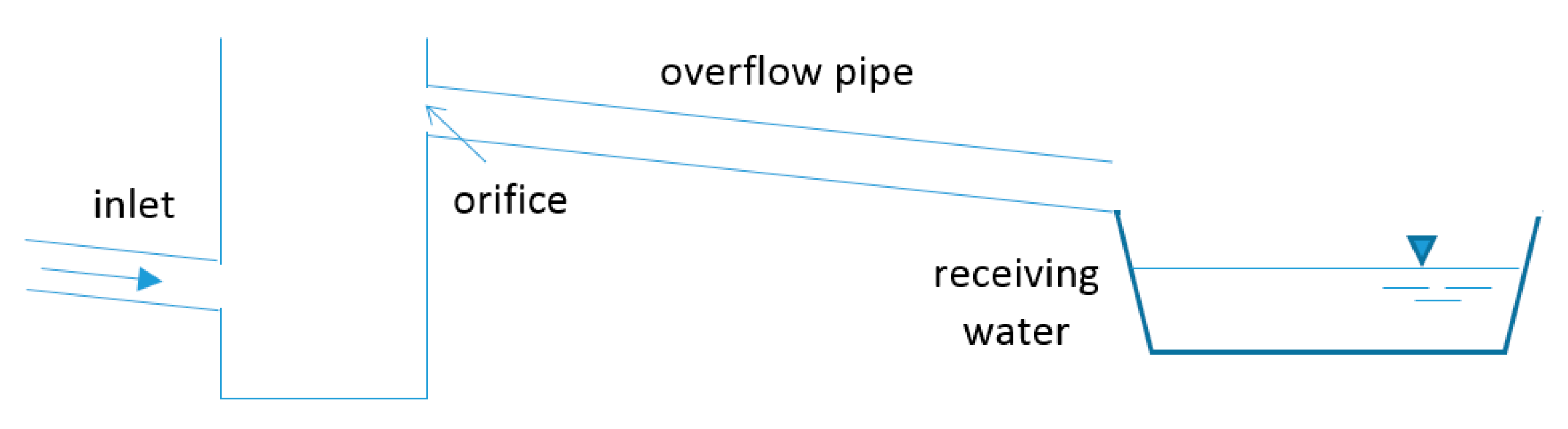
Z (m), as displayed in Figure 3. A circular sharp-crested orifice with diameter d (m) and cross-sectional area, σ (m2), is made at the bottom of the tank. A stationary and uniformly distributed runoff intensity, r (m s−1) corresponding to a runoff discharge R (m3 s−1), is applied over the tank (Figure 3).
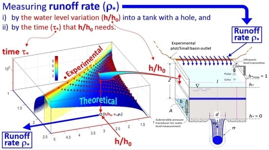
The tank water level is denoted as h (m) and can be measured either by a submersible pressure transducer or by an ultrasonic probe, coupled with a data logger (Figure 3). The latter can be installed at the top of a wide piezometer connected to the water tank, in order to measure the height to which a column of the water rises against gravity, without the disturbance effects at the open water surface caused by the incoming runoff discharge into the tank.
The water level is also expressed in dimensionless terms as h∗ = h/Z. Thus, h∗ = 0 and h∗ = 1 (Figure 3) indicate that the water tank is completely empty or full, respectively. Furthermore, the outflow rate from the hole of the water tank is denoted as v0 (m/s) and the corresponding discharge as Q0 (m3 s−1). The one-dimensional differential continuity equation applied to the infinitesimal volume, dh height (Figure 3), can be written as:
A   d h = ( R μ   σ   v 0 ( h ) )   d t
where t (s) is the time and μ is the discharge coefficient (usually assumed as 0.6 for a perfectly crested orifice) that takes into account the reduction of the discharge velocity due to the viscous behavior of the water (coefficient of velocity) and the reduction of the effective outflow cross-section due to the vena contracta (coefficient of contraction) [36]. Values of the discharge coefficient, μ, which slightly differ from 0.6 could also be taken into account, by considering the unified equation developed by Swamee and Swamee [37] that provides a smooth transition between viscous and potential flows.
Equation (1) states that during a runoff event with constant discharge, R, the water volume exiting the jet by the outlet, in time dt, is equal to the water volume removed from the tank added to that stored in the tank, in the same time dt. In Equation (1), the outflow rate, v0, can be expressed by the well-known Torricelli law, which derives by the conservation of energy [21]:
v 0 ( h ) = 2   g   h
where g (m s−2) is the acceleration due to gravity. The water level gradient can be derived by Equation (1):
d h d t = 1 A   ( R μ   σ   v 0 ( h ) )
For the continuity condition of the flow, v0 (Equation (2)) can also be expressed as a function of the outflow rate, v, as referred to the tank base area, A (Figure 3):
v 0 ( h ) = v ( h )   A μ   σ
Substituting Equation (4) into Equation (1) allows rewriting the water level rate:
d h d t = 1 A   ( R v ( h ) A )
Now, define a characteristic time for the emptying tank process, tc, as the time that the water particle starting from the top water tank needs to cross the entire tank height Z, under steady state conditions and with velocity v = vmax:
t c = Z v m a x
where vmax is the maximum value of v associated with v0 (Equation (4)). Equation (6) shows that, of course, tc also corresponds to the minimum travel time required for the water particle to cross the entire tank height.
The maximum velocity of the water tank level, vmax, can be derived by Equation (4) and by placing h = Z in Equation (2):
v m a x = μ   σ A   v 0 , m a x = μ   σ A   2   g   Z
As expected, Equations (6) and (7) show that the more vmax increases the less the travel time, tc, will be. Dividing the numerator and the denominator on the left side of Equation (5) by the characteristic time tc (Equation (6)), provides:
d h * d τ = 1 v m a x   A ( R v   A )
where τ is the time normalized with respect to tc, while h∗ is the water level, h, normalized with respect to the tank height, Z. Equation (8), which is consistent in regard to a dimensional point of view, can be further simplified as:
d h * d τ = ρ h *
where ρ is the runoff excess intensity, r (m s−1), i.e., R/A, normalized with respect to vmax:
ρ = R A v m a x = r v m a x
and where √h∗ was obtained by substituting into Equation (8) the following ratio:
v v m a x = μ   σ A   2   g   h μ   σ A   2   g   Z = h *
Equation (9) is a more compacted form of the differential flow equation than Equation (1), and it can be usefully considered for the purposes of this study, in order to derive a purely theoretical stage–discharge relationship for measuring input runoff discharges to be directly used in field and in experimental applications, requiring limited calibration, as will be shown. Equation (8) can be integrated, by fixing the initial condition h = h0 for t = t0, or in dimensionless terms:
h * = h * 0 for τ = τ 0
under the reasonable assumption that during the close interval [τ0, τ], which could also fit the normalized time step of water level measurements (τm = τ − τ0), the runoff discharge R (Equation (1)) and the corresponding ρ are time-invariant:
τ 0 τ d τ = h * 0 h * d h * ρ   h *
Equation (13) shows that for ρ = √h∗ a limiting condition occurs, so that the normalized water content asymptotically attains an equilibrium value, which can be derived by imposing h∗ = ρ2.
Two different cases can be distinguished:
(i) ρ ≠ 0. In this case, the integral of Equation (13) can be solved by u-substitution or the reverse chain rule, by putting u = √h∗ and dh∗ = 2 u du, giving:
τ = τ 0 + 2 u 0 u u ρ   u d u
Adding and subtracting ρ in the numerator yields:
τ τ 0 = 2 u u 0 u ρ + ρ u ρ d u = 2 u u 0 d u + 2 u u 0 ρ u ρ d u = 2 ( u 0 u ) + 2 ρ ln | u 0 ρ u ρ |
By substituting back again into Equation (15) u = √h∗, an explicit τ solution can be derived:
τ = τ 0 + 2   ( ρ   ln | ρ h * 0 ρ h * | ( h * h * 0 ) )
(ii) ρ = 0. This case describes the recession of the emptying tank process, starting at the end of the runoff process, τr, i.e., τ0 = τr and h*0 = h*r, with h*r denoting the normalized water level at the end of the runoff process, when ρ = 0. Thus, Equation (13) can be rewritten as:
τ r τ d τ = h * h * r d h * h *
which, once integrated, provides the following explicit solution in τ or in h∗, respectively:
τ = τ r + 2   ( h * r h * )
h * = ( h * r τ τ r 2 ) 2
According to the dimensionless variables introduced, Equation (18) makes it possible to derive the time required for the zero flux condition, τzf, i.e., for h∗ = 0, when the tank is completely empty:
τ z f = τ r + 2   h * r
that can be expressed dimensionally by using Equations (6) and (7) and assuming τr = 0, yielding the well-known formula:
t z f = 2 μ g A σ h r
Equations (20) and (21) are not strictly useful towards the objectives of this work since they can be applied at the end of the runoff process, when the runoff intensity, r, equals zero. However, they can be used to test how well the runoff measurement device performs, since it makes it possible to check that when the water level is h = h∗ = 0, the time that passes from the initial water level, i.e., hr, to the zero flux condition would be tzf = τzf tc.
It should be noted that Equation (9) differs from the well-known linear reservoir model, commonly used in catchment hydrology, which assimilates the catchment to a reservoir. In fact, in that case, it is assumed that the water volume stored in the reservoir linearly varies with the output discharge, according to a constant k(t), which is also related to the response time of the catchment [38,39]. This assumption would provide a different form of the differential equation and its solution, which are reported in a dimensional form here, by assuming as initial condition v = 0, for t = 0:
d t = k r v d v
v ( t ) = r   ( 1 e t / k )
The linearity assumption in Equations (22) and (23) is an approximation. This is equivalent to assuming that the superposition principle could be applied to both the runoff generation process in the catchment hydrology, and to the water tank behavior, if referring to this study. Actually, both the runoff generation process, especially at the hillslope scale [40,41], and the water reservoir (the latter because of introducing Torricelli’s law), are non-linear. Therefore, in both cases, the superposition principle is not satisfied and thus cannot be applied. With reference to the non-linear water tank considered in this study, by using the Laplace transform, Equation (9) could be linearized; however, this issue is beyond the objective of this work and does not further contribute to the results that will be shown.
In order to derive the normalized runoff discharge, ρ, i.e., the runoff intensity (Equation (10)), Equation (16) needs to be rewritten as follows:
ρ = τ m 2 + h * h * 0 l o g ( ρ h * 0 ρ h * )
that provides an implicit ρ solution for a fixed normalized time τm spent from the initial condition h*0 to the actual condition h∗. Thus, the time tm = (tt0) = τm tc represents the time step of water level measurements, i.e., the time that the water level h0, at t = t0, needs to achieve the current value h, at t = t0 + tm. Of course, tm, i.e., τm, needs to be established according to the desired resolution of the indirect water level measurement device (Figure 3).
Equation (24) shows that the output variable ρ, depends on three parameters τm, h∗, and h*0, which complicate a graphical illustration of the non-linear water tank performance. However, in Equation (24), the ρ dependence can be reduced to two parameters by dividing the left and right side by √h*0:
ρ h * 0 = τ m 2 h * 0 + h * h * 0 1 l o g   ( ρ h * 0 1 ρ h * 0 h * h * 0 )
By introducing the following three dimensionless groups:
ρ * = ρ h * 0
H * = h * h * 0
τ * = τ m 2 h * 0 = τ τ 0 2 h * 0
Equation (25) can be rewritten, showing a ρ∗ dependence on only two dimensionless groups, H∗ and τ∗:
ρ * = τ * + H * 1 l o g ( ρ * 1 ρ * H * )
thus making a better graphical parametrization than Equation (24) possible. It should also be noted that Equation (29) differs from the stage–discharge relationships mentioned in the introduction section, where relationships between water level and runoff discharge were found. Indeed, in Equation (29) no calibration coefficients appear, and the runoff discharge is related to the water level variation, H∗, rather than the water level. Therefore, it could be more appropriate denoting Equation (29) as a stage variation–discharge relationship, as in this subsection title.
The present approach is similar to that recently applied to the soil [42], which was also treated as a non-linear reservoir in order to derive an analytical solution for the Richards equation, under gravity-driven infiltration and constant rainfall intensity. Here, such a similar approach has been reformulated, according to a different characteristic time of the water tank and to different input and output dimensionless groups. In fact, for the soil, the known input was the rainfall intensity and the soil water content, miming the water tank level, needed to be determined; whereas in the present methodology, the input is the water level variation, and the output (i.e., the unknown) is the runoff input discharge at the outlet.

2.2. Range of Values of the Involved Parameters and Stage–Discharge Plot

In order to set a reliable range of variability of the involved dimensionless groups H∗, ρ∗, and τ∗, Table 1 and Table 2 report examples of the ranges of variability of the geometric and hydraulic original variables, respectively, by fixing their assumed extremes (see min and max values). Of course, the lower the range of the input discharge, the cheaper the tank size and cost will be.
For example, a high value of the maximum height Z of the tank was fixed (
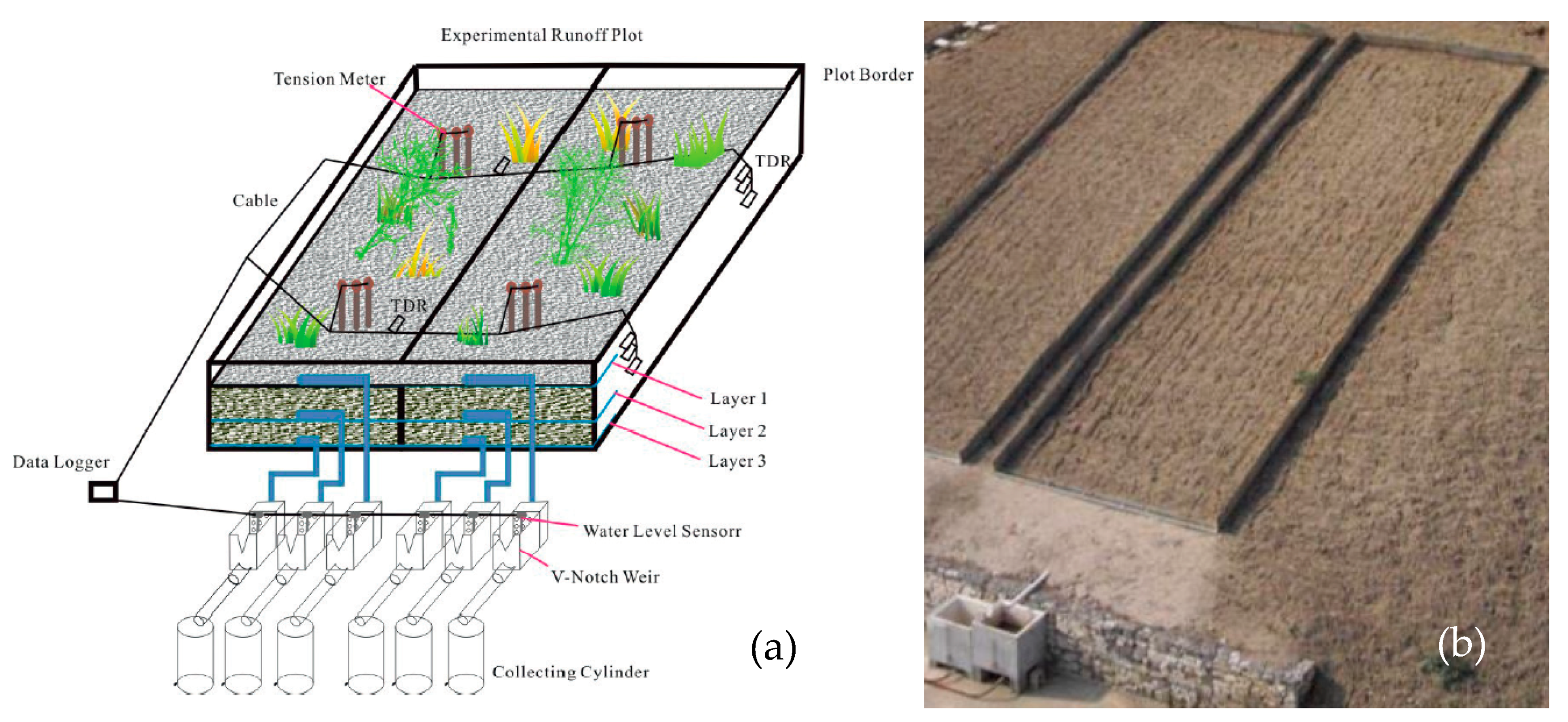
Z = 4 m). This could make measuring runoff costly, because of the high excavation costs and the large size of the water tank. However, it would be reliable once installed downstream from a check dam where a drop in elevation occurs or more properly at the experimental plots’ outlet (Figure 1).
Table 1 shows that the outlet hole diameter also varied in a wide range (0.02–0.3 m), in order to extend the range of variability of runoff measurements.
Once the range of variability of the involved original variables was established, those of the corresponding output dimensionless groups were determined and reported in Table 3, which also includes those rounded ranges considered in the application of Equation (29).
According to these rounded ranges (
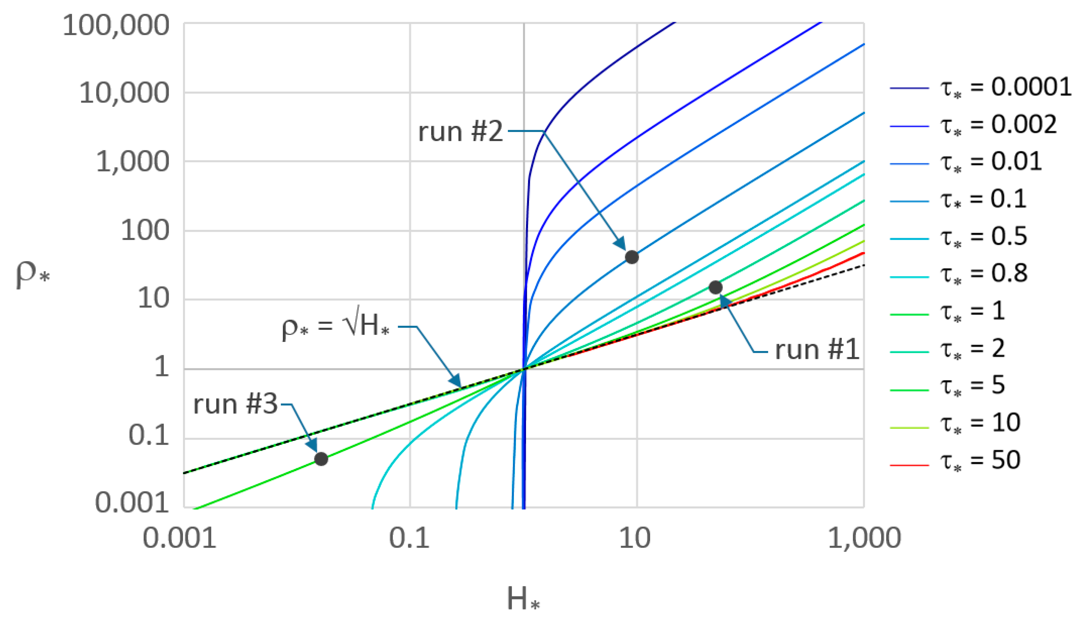
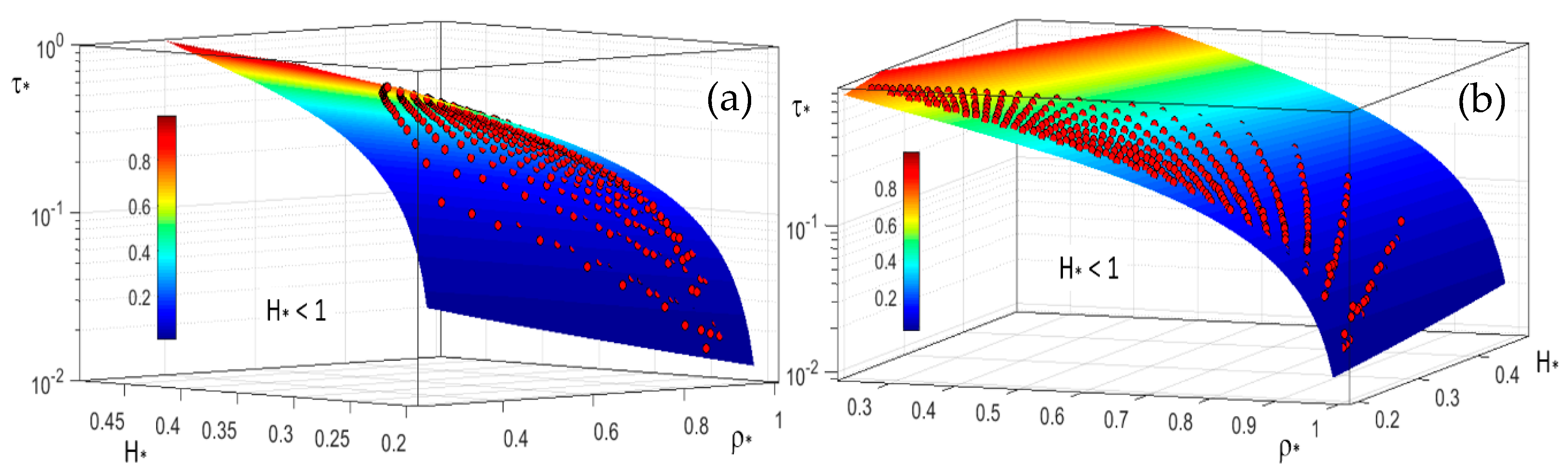
Table 3) and by using Equation (29), the output variable, ρ∗, which makes it possible to estimate the runoff intensity, was plotted in Figure 4, versus H∗, with τ∗ as a parameter, which also varied according to its range of variability (Table 3).
Figure 4 shows that all of the curves pass from H∗ = ρ∗ = 1, according to the fact that when no difference between h*0 and h∗ is measured (H∗ = 1), the outlet process is steady state and the corresponding runoff intensity can be calculated by the well-known equation, r = μ σ/A √(2 g h0). Thus, under this condition, ρ∗ equals the unity (Equations (10) and (26)). Figure 4 also shows that for any τ∗, the ρ∗(H∗) curves monotonically increase, indicating, as expected, that for a fixed time step measurement, tm, i.e., τ∗, at increasing H∗ the runoff intensity also increases. Moreover, for a fixed H∗, (i.e., for a fixed antecedent and actual water levels), runoff intensity becomes higher and higher, as the time step measurement, τ∗, decreases. This latter behavior also agrees with what is expected.
It should be noted that the tank design has to be performed according to the runoff regime of the studied plot/basin. In fact, as previously observed, tank volumes and hole diameters that are too small would not make it possible to measure the runoff intensity by the water level ratio, H∗, since the tank would get full too quickly. On the contrary, tank volumes and hole diameters that are too large would not make it possible to measure the runoff intensity by Equation (29), because the variation of the water level ratio, H∗, would be too small. These two latter extreme behaviors are described in Figure 4, by the vertical and almost horizontal branches of the plotted curves, respectively.

2.3. Water Reservoir Design

Some considerations can help detect the optimal water tank design according to the suggested procedure, for different runoff regimes. In fact, for an assigned tank dimension, it is easy to derive the minimum and maximum runoff rate, and the derived relationships that can be used in regard to the tank design. In particular, the maximum outlet discharge from the tank hole, Q0,max, and the maximum storage discharge, Q0,st, and their sum, Rmax, can respectively be expressed as:
Q 0 , m a x = v 0 , m a x   σ = μ   σ   2   g   Z
Q s t , m a x = A   Z t m .
R m a x = Q 0 , m a x + Q s t , m a x = μ   σ   2   g   Z + A   Z t m .
whereas, by assuming a minimum water level equal to a very low fraction of Z, α Z, with α = 1%–2%, the corresponding minimum values, Q0,min, Qst,min, and Rmin, can be derived:
Q 0 , m i n = μ   σ   2   g   α   Z
Q s t , m i n = A   α   Z t m
R m i n = Q 0 , m i n + Q s t , m i n = μ   σ   2   g   α   Z + A   α   Z t m
By using Equations (32) and (35), and by imposing the time step measurement, tm, derived from them as equal, the following relationship of the outlet cross-sectional area, σ, can be obtained:
σ = α   R m a x R m i n μ   2   g   Z   ( α α )
Equation (36) can also be rewritten by considering the much more useful hole diameter, d (mm), rather than the hole cross-sectional area, σ:
d = 1000 2 3 / 4 α   R m a x R m i n   μ   π   g   Z   ( α α )
Table 4 reports the minimum and maximum values of the runoff discharge, Rmax and Rmin, respectively, for three considered study cases, run #1, run #2, and run #3, within which the runoff discharge must be measured according to its temporal variability.
For these Rmax and Rmin values, and by assuming a fraction of the tank height α = 0.01, Figure 5 graphs the hole’s cross sectional area, σ, and the corresponding hole diameter, d, according to Equation (36) (Figure 5a) and Equation (37) (Figure 5b), respectively.
Figure 5 shows that a water tank satisfying the R range of variability can be designed by a multitude of pairs (d, Z). However, most of their values are out of the reasonable assumed ranges and can correspond to time step water level measurements, tm, which do not necessarily match those that can be assumed in practice. In the following section, applications of the suggested procedure to measure the runoff discharge are performed and tm values for the three runs are first calculated.

3. Theoretical and Experimental Applications

3.1. Theoretical Applications

Assume that the geometric characteristics of the three runs are those reported in Table 4. For the selected base area, A, hole diameter, d, and tank height, Z, the time step water level measurements, tm, can be calculated by Equation (32) or by Equation (35). In the following, tm is derived by Equation (32):
t m = t t 0 = A   Z R m a x μ   σ   2   g   Z
Table 5 reports the tm values obtained by Equation (38), for the considered three runs. These values vary between 4.3 s and 15 s and seem suitable to be recorded by a submersible pressure transducer data logger, thus, they will be considered as a constant in the following. However, as observed above, different pairs (d, Z) can be selected, in order to match the desired tm, for a fixed base area, A.
For the fixed tm, let us assume that water level measurements provide the initial and actual water levels, h0 and h, reported in Table 5, where the corresponding normalized values h*0 and h0 are also indicated. In order to estimate the corresponding runoff discharge, the h*0 and h∗ values make it possible to calculate the first dimensionless group, H∗ = h/h0, considered in Equation (29).
By using Equation (7) the corresponding vmax was also calculated and reported in Table 5. Noticeably, run #3 corresponds to an empty process of the water tank, since H∗ is less than one, because the initial value (h0 = 0.5 m) was assumed higher than the actual value (h = 0.008 m).
In order to calculate τ∗ (Equation (28)), Table 6 reports the characteristic time, tc (Equation (6)), together with the ρ∗ parameter (Equation (29)). Once, ρ∗ is calculated, by using Equations (10) and (26), subsequently ρ and the runoff discharge, R, can also be calculated, respectively. Results are reported in Table 6, where together with the runoff discharge, R, the runoff intensity r (m s−1) and the runoff discharge per unit km2 (mm h−1 km−2), were also computed.
A comparison between Table 6 and Table 4 shows that for run #1 and run #2, R is in between the assumed range (RminRmax), whereas it is not for run #3 (R = 0.003 m3 s−1). This result is justified by the fact that, for run #3, the actual h value (0.003) was also assumed to be out of the fixed range (0.008–4, Table 2). Of course, this circumstance does not limit the reliability of the suggested procedure to calculate the runoff discharge, R, since Equation (29) is of general validity, and the suggested ranges of variability of the involved parameters, previously set, only guide a suitable design procedure.
If the hole of the tank was made at the side of the tank, rather than at the bottom, the water level could be measured by an ultrasonic probe installed at the top of the tank (Figure 3) and a dead volume could be easily and properly assigned to the tank volume. The latter is easier to apply because it does not require too high of a drop in elevation, which would be necessary for the hole made at the bottom of the tank. Furthermore, the hole made in the front face of the tank allows designating a dead volume at the tank bottom, where the solid volume can take place. The latter is particularly required when the investigated area is expected to have high levels of soil erosion and sediment yields [43] or when for low-gradient determining high sediment channels, financial constraints, and lack of technical expertise do not allow using traditional flumes and weirs.
For example, for run #2, assuming a small tributary basin, with area S = 0.3 ha and a soil erosion rate, SE = 1 mm year−1, the tank height should be increased by Ze = 10 ER·S/A = 0.75 m, where 10 is the unit conversion factor that makes it possible to express S in (ha), SE in (mm year−1), in order to obtain the additional tank height (m). Thus, the total height would be Z + Ze = 2.75 m, with a depth of the hole under Z = 2 m below the top of the tank. Of course, Ze computation highly depends on the frequency of maintenance that was assumed as once a year in this example.
If Ze is considered, water depth measurements would be modified accordingly. Moreover, it needs to be considered that the sediment, if underestimated, could fill entirely the reservoir disabling the measurement of the discharge, but also if the sediment begins to exit by the hole, the hole area would be modified invalidating the discharge measurement.
In order to test the runoff discharge results of the three runs reported in Table 6, the pairs (H∗, ρ∗) for the corresponding τ∗ values, are plotted in Figure 6, showing the reliability of the indirect runoff discharge measurements.
The water balance was checked by verifying that the inlet runoff volume, Vr, has to balance the outlet volume from the hole, V0, and that stored in the tank, Vst, in the time step water level measurements, tm. The latter two can be easily calculated numerically by considering the water level temporal variation provided by Equation (16) and, just for V0, the v(h) function derived by Equations (2) and (4):
V s t = i = 1 n i ( h i h i 1 ) = h i h 0
V 0 = i = 1 n i 0.5   ( v i + v i 1 ) ( t i t i 1 )
where ni is the number of intervals in which the water level variation, hh0, in the time tm, was subdivided, hi and hi−1 are the water level calculated by Equation (16) at the time ti and ti−1, respectively, and where vi and vi−1 are the corresponding outflow rates (Equations (2) and (4)).
Figure 6 shows the results for each of the three runs, where the volume flowing out from the tank, V0, and the volume stored in the tank, Vst, versus the time are plotted. This representation provides more information than the lumped results illustrated in Figure 4 and allows the water balance to be gradually checked.
For example, Figure 6 shows that storage and outflow volume are distributed well in run #1, whereas for run #2, during the time step, tm, most of the runoff volume is stored in the tank and, compared to run #1, the water volume drained by the hole tank is much less. For run #3, Figure 6 shows that the storage volume, Vst, is negative, since the water level decreases during the time step of measurements (H∗ < 1).
Interestingly, in all three scenarios the slope of the straight volume line derived by the sum of the runoff volume drained by the hole and that stored in the tank (green lines in Figure 6), matches the runoff intensity, r, estimated by the suggested procedure, displayed in the same figure and reported in Table 6. For the three considered cases, this latter occurrence verifies the water balance and suggests that this physically based procedure, characterized by small uncertainty, could be a promising method to accurately measure the runoff discharge for different purposes.
Finally, it should be observed that for high variability of runoff discharge, and depending on large field space availability, installing two or more tanks in a series could be suggested. The latter in order to designate different tank geometries that could be able to collect from low to moderately high discharge data, in order to not increase too much building costs because of the big size that the water tank design could require.

3.2. Experimental Application

In order to experimentally test the suitability of the suggested device to be used for measuring a constant input discharge from water level variations, experimental laboratory measurements were performed for a small water tank (l = 0.275 m, b = 0.378 m, Z = 0.193 m, Figure 7a), which because of its simplicity, truly reproduces the assumptions on which the model is based. A vertical baffle was inserted into the tank to limit the disturbance effect next to the water level measurements. Moreover, in order to clearly read the water level, by means of a meter placed on the inner side of the tank, water into the tank was dyed blue (Figure 7a).
For the considered tank size (l, b, and Z) and for the considered input discharge range (0.02–0.15 l/s), measured by a water flow meter, the water tank design suggested a hole size d = 11.1 mm.
Under time-variable hole outflow, an emptying process was performed for a low constant input discharge, Rm = 0.0294 l/s, starting from a water level h0 = 17 cm to h = 4 cm; whereas, a filling process was simulated for a high constant input discharge, Rm = 0.1195 l/s, starting from a water level h0 = 4 cm to h = 17 cm. In both cases, n = 27 cumulated water levels, with step 0.5 cm, were measured.
In order to check the procedure for many possible combinations of the pairs (h0, h) and (t0, t), water level data were disaggregated. Thus, for both processes, the combinations N = n (n−1)/2 = 351 of disaggregated data were considered (Table 7).
For both processes, the runoff coefficient, μ, was calculated by minimizing the standard error of the estimate, SEE, between the empirical (tt0)m and that calculated by the theoretical relationship (tt0)c = (τ − τ0) tc (Equation (16)):
S E E = i = 1 N ( ( t t 0 ) m ( t t 0 ) c ) 2 N 1
Results are reported in Table 7 and show that the self-built sharp-crested orifice (Figure 7c) provided a runoff coefficient greater than that commonly assumed (μ = 0.6), probably because of the non-perfectly crested orifice. More importantly, the runoff coefficient did not show a water level dependency, since the two constant μ values (0.733 and 0.671), as the first check of the procedure, made it possible to very positively compare the measured (tt0)m and the calculated (tt0)c values (Figure 8a). On the contrary, the discharge coefficient showed a dependence by the input discharge, since it resulted as higher for the emptying process than for the filling one, according to the fact that a higher input discharge provides higher losses (μ = 0.671) than the lower input discharge (μ = 0.733).
Table 7 also reports the corresponding SEE values that resulted in a lower value for the emptying process (1.72 s) than for the filling one (11.24 s).
When using this device, the unknown variable is the input discharge, R; therefore, the latter was also calculated (Rc) by using Equation (29) and its frequency distribution is reported in Figure 8b, whereas the corresponding Rc statistics are reported in Table 7. Results show that in both cases the mean values of Rc are very close to the measured one, Rm. However, the coefficient of variation CV was much higher for the emptying process than for the filling process, as can also be observed by the corresponding frequency distribution (Figure 8b).
For the amount of experimental measurements, the corresponding triplet of values (H∗, ρ∗, and ρ∗) are also plotted in two different 3D views in Figure 9a,b for H∗ < 1, and in Figure 10a,b for H∗ > 1, where Equation (29), fitting the data well, was also graphed. Figure 9 and Figure 10 provide a more general performance of the stage variation–discharge relationship than Figure 4, and they could be implemented in a data-logger software application, so to collect both water levels and flow discharge data. In Figure 10, the vertical surface (in yellow) corresponding to the limiting condition is also illustrated.
An error analysis was performed by calculating the relative error, RE, based on the discharge as a function of the normalized water level, H∗ = h/h0 (Figure 8c). Interestingly, Figure 8c shows that for both the emptying and the filling processes, RE in the input discharge estimate, Rc, decreases at H∗ decreasing (for H∗ < 1) or increasing (for H∗ > 1), whereas RE increases next to H∗ = 1. The latter means that when the actual water level, h, is close to the antecedent water level, h0, the input discharge by Equation (29) is not estimated well and that for such conditions the common steady state relationship should be used (r = μ σ /A √(2 g h0)). Moreover, it is confirmed that for the emptying process, RE in Rc estimation is much higher for the emptying process than the filling one.
According to the above considerations, another error analysis was performed by considering the hole data set, N = 351, and by excluding the data next to the steady state condition corresponding to 0.8 < H∗ < 1 and to 1 > H∗ > 2, for the emptying and the filling processes, respectively.
Results are reported in Table 8, which clearly shows that for the filling process, if the whole data set is considered (H∗ > 1), RE is very low (±3%) in 90% of measurements; this further increases for the limited data set (N = 98%). For the emptying process and for the limited data set (H∗ < 0.8) the percent of measurements providing a satisfactory RE = ±0.05 remained high (N = 71%). Therefore calculating Rc discharge in emptying conditions, due to larger subjective errors in time measurements, than in filling conditions (since tm emptying << tm filling), is not recommended. However, the latter issue could be improved by measuring the pairs time-water level by probes.

4. Conclusions

This work proposed a theoretically based stage–discharge relationship of a non-linear water reservoir with a hole made at the bottom or at the side of the tank, which requires a limited calibration of the physical meaningful discharge coefficient characteristic of the hole. The derived solution makes it possible to measure the inlet runoff discharge (i) starting just from the water level variation into the tank and (ii) from the time that the water level variation requires. Due to the large size and the corresponding high drop in elevation that the water tank could require for high discharges, the suggested device, and the corresponding stage–discharge relationship, is better aimed at limited runoff discharges measured by experimental plots or small basins.
The main advantages of the proposed device are: (i) it requires limited calibration of the just one physical meaningful discharge coefficient; (ii) it cannot be affected by free and submerged flow conditions; (iii) it could be very cheap (for low discharges); and (iv) it requires very limited maintenance.
A water reservoir design that makes it possible to detect the main geometrical characteristics of the tank, according to a desirable variability range of the runoff discharge, was suggested.
For three theoretical applications, the mass water balance was checked, which may help in understanding the reliability of the proposed procedure.
For a simple, small water tank that truly reproduces the assumptions on which the model is based, the suitability of this solution was also experimentally tested. Results showed that the suggested device could be applied in practical conditions, with acceptable errors.
However, more experimental analyses are needed that could be focused on the influence of the water level and input discharge on the runoff coefficient, in order to further reduce the errors in the input discharge estimation. It should be noted that the observed water level measurements, which were used to estimate input discharge, could be affected by slight subjective errors; these could be fixed by measuring times and water levels by probes connected to a data-logger.

Acknowledgments

The Author wishes to thank Santino Orlando for building the water tank orifice and the four anonymous reviewers for the helpful comments and suggestions made during the revision stage.

Conflicts of Interest

The author declares no conflicts of interest.

List of Symbols

A=base area of the tank[L2]
b=base side of the tank[L]
d=hole diameter[L]
g=acceleration due to gravity[L T−2]
h=tank water level[L]
h0=tank water level at the antecedent condition (t = t0)[L]
h=tank water level normalized with respect to Z
h*r=tank water level normalized with respect to Z corresponding to the time τr
h*0=tank water level at the antecedent condition normalized with respect to Z.
H=ratio between h∗ and h*0 (i.e., between h and h0)
k=constant of the linear reservoir model[T]
l=base side of the tank[L]
ni=number of intervals in which the water level variation, h∗ − h*0, was subdivided.
n=number of cumulated water levels measurements
N=number of disaggregated water levels measurements
Qst,max=maximum value of the discharge stored in the tank[L3 T−1]
Qst,min=minimum value of the discharge stored in the tank[L3 T−1]
Q0=outflow rate from the bottom of the tank[L3 T−1]
Q0,max=maximum value of Q0[L3 T−1]
Q0,min=minimum value of Q0[L3 T−1]
r=runoff intensity[L T−1]
R=runoff discharge[L3 T−1]
Rc=calculated runoff (input) discharge[L3 T−1]
Rm=measured runoff (input) discharge[L3 T−1]
Rmax=maximum value of the runoff discharge[L3 T−1]
Rmin=minumum value of the runoff discharge[L3 T−1]
S=catchment area[L2]
SE=soil erosion[L T−1]
t=time[T]
tc=characteristic time of the empting tank process[T]
tm=time step of the water level measurements[T]
(tt0)c=calculated time step of the water level measurements[T]
(tt0)m=measured time step of the water level measurements[T]
tzf=time corresponding to the zero flux condition from the end of the runoff
process[T]
t0=time at h = h0[T]
v=outflow rate at the bottom of the tank corresponding to the tank base area[L T−1]
vmax=maximum value of v[L T−1]
v0=outflow rate at the bottom of the tank[L T−1]
v0,max=maximum value of v0[L T−1]
Vst=volume stored in the tank per unit tank area[L]
V0=volume flowing out from the tank per unit tank area[L]
Vr=runoff volume V0 + Vst[L]
Z=height of the tank[L]
Ze=additional water tank height to consider yearly sediment yield[L]
α=fraction of the maximum tank water level (0.01–0.02)
µ=discharge coefficient of the orifice
ρ=runoff intensity normalized with respect to vmax.
ρ∗=dimensionless group to estimate the runoff intensity (Equation (21a))
σ=cross-sectional area of the hole at the bottom of the tank[L2]
τ=time normalized with respect to tc.
τm=time step of the water level measurements normalized with respect to tc.
(τ − τ0)c=calculated time step of the water level measurements normalized with respect to tc.
(τ − τ0)m=measured time step of the water level measurements normalized with respect to tc.
τr=time normalized with respect to tc corresponding to the end of the runoff process
τzf=time normalized with respect to tc corresponding to the zero flux condition
τ0=time normalized with respect to tc corresponding to the initial water level
τ∗=dimensionless group corresponding to the time step of water level measurements (Equation (21c))

References

  1. Tazioli, A. Experimental methods for river discharge measurements: Comparison among tracers and current meter. Hydrol. Sci. J. 2011, 56, 1314–1324. [Google Scholar] [CrossRef]
  2. Tauro, F.; Selker, J.; van de Giesen, N.; Abrate, T.; Uijlenhoet, R.; Porfiri, M.; Manfreda, S.; Kelly Caylor, K.; Moramarco, T.; Benveniste, J.; et al. Measurements and Observations in the XXI century (MOXXI): Innovation and multidisciplinarity to sense the hydrological cycle. Hydrol. Sci. J. 2018, 63, 169–196. [Google Scholar] [CrossRef] [Green Version]
  3. Lee, J.; Shin, H.; Ahn, J.; Jeong, C. Accuracy Improvement of Discharge Measurement with Modification of Distance Made Good Heading. Adv. Meteorol. 2016, 2016, 1–9. [Google Scholar] [CrossRef]
  4. Ranzi, R.; Bacchi, B.; Grossi, G. Runoff measurements and hydrological modelling for the estimation of rainfall volumes in an Alpine basin. Q. J. R. Meteorol. Soc. 2003, 129, 653–672. [Google Scholar] [CrossRef]
  5. Lenzi, A.; Mao, L.; Comiti, F. Effective discharge for sediment transport in a mountain river: Computational approaches and geomorphic effectiveness. J. Hydrol. 2006, 326, 257–276. [Google Scholar] [CrossRef]
  6. Bagarello, V.; Ferro, V. Analysis of soil loss data from plots of differing length for the Sparacia experimental area, Sicily, Italy. Biosyst. Eng. 2010, 105, 411–422. [Google Scholar] [CrossRef]
  7. Viglione, A.; Chirico, G.B.; Komma, J.; Woods, R.; Borga, M.; Blöschl, G. Quantifying space–time dynamics of flood event types. J. Hydrol. 2010, 394, 213–229. [Google Scholar] [CrossRef]
  8. Picco, L.; Mao, L.; Rigon, E.; Moretto, J.; Ravazzolo, D.; Delai, F.; Lenzi, M.A. An update of the magnitude–frequency analysis of Rio Cordon (Italy) bedload data after 25 years of monitoring. Erosion and Sediment Yields in the Changing Environment. In Proceedings of the A Symposium Held at the Institute of Mountain Hazards and Environment 2012, Chengdu, China, 11–15 October 2012. [Google Scholar]
  9. Carollo, F.G.; Di Stefano, C.; Ferro, V.; Pampalone, V. New stage-discharge equation for the SMBF flume. J. Irrig. Drain. Eng. 2016, 142, 04016005. [Google Scholar] [CrossRef]
  10. Romano, N.; Nasta, P.; Bogena, H.; De Vita, P.; Stellato, L.; Vereecken, H. Monitoring Hydrological Processes for Land and Water Resources Management in a Mediterranean Ecosystem: The Alento River Catchment Observatory. Vadose Zone J. 2018, 17, 180042. [Google Scholar] [CrossRef] [Green Version]
  11. Yang, L.; Song, X.; Qiao, Y. Water Cycle Process Research: Experiments and Observations. In Hydrology of Artificial and Controlled Experiments; Liu, J.-F., Gu, W.-Z., Eds.; IntechOpen: London, UK, 2017. [Google Scholar] [CrossRef] [Green Version]
  12. McMillan, H.; Freer, J.; Pappenberger, F.; Krueger, T.; Clark, M. Impacts of uncertain river flow data on rainfall-runoff model calibration and discharge predictions. Hydrol. Process. 2010, 24, 1270–1284. [Google Scholar] [CrossRef]
  13. Di Baldassarre, G.; Montanari, A. Uncertainty in river discharge observations: A quantitative analysis. Hydrol. Earth Syst. Sci. 2009, 13, 913–921. [Google Scholar] [CrossRef] [Green Version]
  14. Corato, G.; Moramarco, T.; Tucciarelli, T. Discharge estimation combining flow routing and occasional measurements of velocity. Hydrol. Earth Syst. Sci. 2011, 15, 2979–2994. [Google Scholar] [CrossRef] [Green Version]
  15. Peña-Arancibia, J.L.; Zhang, Y.; Pagendam, D.E.; Viney, N.R.; Lerat, J.; van Dijk, A.I.J.M.; Vaze, J.; Frost, A.J. Streamflow rating uncertainty: Characterisation and impacts on model calibration and performance. Environ. Model. Softw. 2015, 63, 32–44. [Google Scholar] [CrossRef]
  16. Zeroual, A.; Meddi, M.; Assani, A.A. Artificial Neural Network Rainfall-Discharge Model Assessment under Rating Curve Uncertainty and Monthly Discharge Volume Predictions. Water Resour. Manag. 2016, 30, 3191–3205. [Google Scholar] [CrossRef]
  17. Osorio, A.L.N.A.; Reis, D.S. A Bayesian Approach for the Evaluation of Rating Curve Uncertainties in Flood Frequency Analyses. In World Environmental and Water Resources Congress 2016; American Society of Civil Engineers: Reston, VA, USA, 2016; pp. 482–491. [Google Scholar] [CrossRef]
  18. Steinbakk, G.H.; Thorarinsdottir, T.L.; Reitan, T.; Schlichting, L.; Hølleland, S.; Engeland, K. Propagation of rating curve uncertainty in design flood estimation. Water Resour. Res. 2016, 52, 6897–6915. [Google Scholar] [CrossRef]
  19. Walkowiak, D.K. (Ed.) ISCO Open Channel Flow Measurement Handbook; Teledyne Isco: Lincoln, NE, USA, 2006. [Google Scholar]
  20. Dobriyal, P.; Badola, R.; Tuboi, C.; Hussain, S.A. A review of methods for monitoring streamflow for sustainable water resource management. Appl. Water Sci. 2017, 7, 2617–2628. [Google Scholar] [CrossRef] [Green Version]
  21. Torricelli, E. Opera Geometrica, Amatoris Masse & Laurentij de Landis; Svperiorvm Permissv: Florence, Italy, 1644. [Google Scholar]
  22. Welber, M.; Le Coz, J.; Laronne, J.B.; Zolezzi, G.; Zamler, D.; Dramais, G.; Hauet, A.; Salvaro, M. Field assessment of noncontact stream gauging using portable surface velocity radars (SVR). Water Resour. Res. 2016, 52, 1108–1126. [Google Scholar] [CrossRef] [Green Version]
  23. Tan, M.L.; Latif, A.B.; Pohl, C.; Duan, Z. Streamflow modelling by remote sensing: A contribution to digital earth. IOP Conf. Ser. Earth Environ. Sci. 2014, 18, 012060. [Google Scholar] [CrossRef] [Green Version]
  24. Tauro, F.; Olivieri, G.; Petroselli, A.; Porfiri, M.; Grimaldi, S. Flow monitoring with a camera: A case study on a flood event in the Tiber river. Environ. Monit. Assess 2016, 188, 1–11. [Google Scholar] [CrossRef]
  25. Perks, M.T.; Dal Sasso, S.F.; Hauet, A.; Le Coz, J.; Pearce, S.; Peña-Haro, S.; Tauro, F.; Grimaldi, S.; Hortobágyi, B.; Jodeau, M.; et al. Towards harmonization of image velocimetry techniques for river surface velocity observations. Earth Syst. Sci. 2019, 2019, 1–20, In review. [Google Scholar] [CrossRef] [Green Version]
  26. Fread, D.L. Computation of stage-discharge relationships affected by unsteady flow. JAWRA J. Am. Water Resour. Assoc. 2007, 11, 213–228. [Google Scholar] [CrossRef]
  27. Ghasemzadeh, F.; Kouchakzadeh, S.; Belaud, G. Unsteady Stage-Discharge Relationships for Sharp-Crested Weirs. J. Irrig. Drain. Eng. 2020, 146, 04020009. [Google Scholar] [CrossRef]
  28. Parshall, R.L. The Improved Venturi Flume. Trans. ASCE 1926, 89, 841–880. [Google Scholar]
  29. Samani, Z.; Jorat, S.; Yousaf, M. Hydraulic Characteristics of a Circular Flume. J. Irrig. Drain. Eng. 1992, 117, 559–567. [Google Scholar] [CrossRef]
  30. Samani, Z.; Magallanez, H. Simple flume for flow measurement in open channel. J. Irrig. Drain. Eng. 2000, 126, 127–129. [Google Scholar] [CrossRef]
  31. Vatankhah, A.R. Stage-Discharge Relationship for Sharp-Crested Rectangular Slit Weirs. J. Irrig. Drain. Eng. 2019, 145, 06019006. [Google Scholar] [CrossRef]
  32. Baiamonte, G.; Ferro, V. Simple Flume for Flow Measurement in Sloping Open Channel. J. Irrig. Drain. Eng. 2007, 133, 71–78. [Google Scholar] [CrossRef]
  33. Bijankhan, M.; Ferro, V. Dimensional analysis and stage-discharge relationship for weirs: A review. J. Agric. Eng. 2017, 48, 1–11. [Google Scholar] [CrossRef]
  34. Rashwan, I.M.H.; Idress, M.I. Evaluation efficiency for mobile as discharge measurement device for partially filled circular channel. Ain Shams Eng. J. 2013, 4, 199–206. [Google Scholar] [CrossRef] [Green Version]
  35. Isenmann, G.; Bellahcen, S.; Vazquez, J.; Dufresne, M.; Joannis, C.; Mose, R. Stage–discharge relationship for a pipe overflow structure in both free and submerged flow. Eng. Appl. Comput. Fluid Mech. 2016, 10, 283–295. [Google Scholar] [CrossRef] [Green Version]
  36. De Marchi, G. Idraulica 1954; Hoepli, U., Ed.; Ulrico Hoepli: Milan, Italy, 1954. (In Italian) [Google Scholar]
  37. Swamee, P.K.; Swamee, N. Discharge equation of a circular sharp-crested orifice. J. Hydraul. Res. 2010, 48, 106–107. [Google Scholar] [CrossRef]
  38. Baiamonte, G.; Agnese, C. Quick and Slow Components of the Hydrologic Response at the Hillslope Scale. J. Irrig. Drain. Eng. 2016, 142, 04016038. [Google Scholar] [CrossRef]
  39. Li, X.; Li, Z. The Application of Linear and Nonlinear Water Tanks Case Study in Teaching of Process Control. ICAESEE IOP Publishing. IOP Conf. Ser. Earth Environ. Sci. 2017, 113, 012165. [Google Scholar] [CrossRef]
  40. Baiamonte, G.; Singh, V.P. Overland Flow Times of Concentration for Hillslopes of Complex Topography. J. Irrig. Drain. Eng. 2016, 142, 04015059. [Google Scholar] [CrossRef]
  41. Baiamonte, G. A rational runoff coefficient for a revisited rational formula. Hydrol. Sci. J. 2020, 65, 112–126. [Google Scholar] [CrossRef]
  42. Baiamonte, G. Analytical solution of the Richards equation under gravity-driven infiltration and constant rainfall intensity. J. Hydrol. Eng. 2020. [Google Scholar] [CrossRef]
  43. Baiamonte, G.; Minacapilli, M.; Novara, A.; Gristina, L. Time Scale Effects and Interactions of Rainfall Erosivity and Cover Management Factors on Vineyard Soil Loss Erosion in the Semi-Arid Area of Southern Sicily. Water 2019, 11, 978. [Google Scholar] [CrossRef] [Green Version]
Figure 1. Examples of experimental plots (a) for runoff measurements (© 2018 Lihu Yang, Xianfang Song and Yunfeng Qiao. Originally published in Water Cycle Process Research [11], under CC BY 3.0 license) and (b) for runoff measurements and sediment yields [6].
Hydrology 07 00023 g001
Figure 2. Sketch of the overflow structure studied by Isenmann et al. [35] (redrawn).
Hydrology 07 00023 g002
Figure 3. Three-dimensional (3D) view of the non-linear water tank where a hole is made at its bottom. Front of the figure refers to the section in the middle of the tank where the hole is made. Two options for water level measurements (submersible and ultrasonic probe) are displayed.
Hydrology 07 00023 g003
Figure 4. Dimensionless group ρ∗, depending on the runoff intensity, versus the dimensionless group H∗ = h∗/h*0, with the normalized time step, τ∗, as a parameter. The figure also plots the equation ρ∗ = √H∗, denoting the limiting condition.
Hydrology 07 00023 g004
Figure 5. Relationship between (a) the hole’s cross sectional area and (b) the corresponding hole diameter, d, versus the tank height, Z. Black dots refer to the applications for the three runs.
Hydrology 07 00023 g005
Figure 6. For (a) run #1, (b) run #2, and (c) run #3, volume stored in the tank, Vst, volume flowing out from the hole, V0, and runoff volume, Vr. Black dots refer to Vr at the time step, tm (Table 5).
Hydrology 07 00023 g006
Figure 7. (a) Experimental water tank, (b) ring where the sharp-crested orifice is inserted, and (c) top and bottom view of the sharp-crested orifice.
Hydrology 07 00023 g007
Figure 8. For the considered emptying (Rm = 0.029 l/s) and filling (Rm = 0.119 l/s) processes, (a) comparison between the time measured, (tt0)m, with that calculated according to the suggested procedure (tt0)c, (Equation (16)); (b) frequency distribution of the calculated input discharge, Rc (Equation (29)); and (c) relative error, RE, versus the normalized water level, H∗.
Hydrology 07 00023 g008
Figure 9. For H∗ < 1, two different 3D views (a) from the bottom and (b) from the top of the stage variation–discharge relationship (Equation (29)). The experimental triplet of values (H∗, ρ∗, and τ∗) (red dots) are plotted.
Hydrology 07 00023 g009
Figure 10. For H∗ > 1, two different 3D views (a) from the bottom and (b) from the top of the stage variation–discharge relationship (Equation (29)). The triplet of the experimental values (H∗, ρ∗, and τ∗) (red dots) and the surface (in yellow), corresponding to the limiting condition, are also plotted.
Hydrology 07 00023 g010
Table 1. Minimum (Min) and maximum (Max) values of the geometric. parameters assumed for the water tank.
ValueA (m2)d (m)σ (m2)Z (m)
Min10.020.00031
Max30.300.07074
Table 2. Minimum (Min) and maximum (Max) values of the hydraulic. parameters assumed for the water tank.
Valuetm (s)h0 (m)H (m)h*0hvmax (m s−1)R (m3 s−1)
Min100.030.030.0080.0080.00030.01
Max903.84.04.03.80.3765
Table 3. Minimum (Min) and maximum (Max) values of derived parameters used in the suggested procedure and runoff results. Bold values refer to H∗ and τ∗ input parameters, and to ρ∗ output parameter, considered in Equations (26)–(28).
MethodValuetc (s)Hττ∗ρρ∗R (m3 s−1)R (m/s)r (mm h−1 km−2)
Calculated (Table 1 and Table 2)Min2.660.0020.00070.00020.00890.00452.47 × 10−68.23 × 10−72.96 × 106
Max14,372533.333.8197.61517,966103,7242.03 × 1042.03 × 1047.29 × 104
Fixed in Figure 4Min-0.001-0.0001-0.01---
Max-1000-50-100,000---
Table 4. For the three runs, runoff discharge ranges, Rmax and Rmin, and water tank geometric parameters.
run #Rmax (m3 s−1)Rmin (m3 s−1)L = B (m)A (m2)d (m)σ (m2)Z (m)
10.1470.006110.150.01771
21.9850.030240.20.03142
30.1610.010110.2120.0351
Table 5. For the three runs, hydraulic parameters of the water tank. Bold values refer to H∗ input parameter considered in Equations (26)–(28).
run #tm (s)h0 (m)H (m)h*0hHvmax (m s−1)
1100.010.50.010.5500.047
24.311.80.10.990.03
3150.50.0080.50.0080.0160.094
Table 6. For the three runs, derived parameters used in the suggested procedure and runoff results. Bold values refer to τ∗ input parameter and to ρ∗ output parameter considered in Equations (26)–(28).
run #tc (s)ττρρR (m3 s−1)R (m/s)r (mm h−1 km−2)
121.290.4702.4415.451.540.0730.0730.261
267.750.0630.142.1713.341.5750.3941.417
310.611.41410.0510.0360.0030.0030.012
Table 7. For the considered emptying and filling processes, h range, runoff discharge, R, and runoff coefficient, μ, and corresponding main statistics.
Processh Range (cm)Rm (l s−1)μnNSEE (t)Mean
Rc (l s−1)
SD
Rc (l s−1)
CV (Rc)SEE(Rc)
emptying17–40.02940.733273511.720.02990.00440.1470.0019
filling4–170.11950.67111.240.11810.00190.0160.0024
Table 8. For the considered emptying and filling processes, sample size of the disaggregated data for the whole data set and for the data set limited by H∗ ranges.
ProcessH∗ BoundNRE RangeNN (%)H∗ BoundNRE RangeNN (%)
emptying<1351±0.8350100%<0.8250±0.8250100%
±0.534398%±0.1524598%
±0.333796%±0.123393%
±0.231991%±0.0822088%
±0.127879%±0.0517871%
±0.0520358%±0.0311646%
filling>1351±0.09351100%>290±0.0990100%
±0.0533495%±0.0590100%
±0.0432693%±0.0490100%
±0.0331590%±0.038898%
±0.0227779%±0.027887%
±0.0119556%±0.015763%

