1. Introduction
The use of pedotransfer functions is seen as a great advantage since measuring hydraulic properties, such as soil water characteristic curves (SWCCs) and hydraulic conductivity, can be time-consuming and costly. Pedotransfer functions (PTFs) estimate soil hydraulic properties using routinely measured soil properties, such as soil texture, bulk density, particle size distribution, or porosity. By compiling and analysing a large quantity of measured soil data, a relationship can be developed thus creating a PTF.
Historically, PTFs were established with natural, native soil in mind rather than engineered substrates such as Low Impact Development (LID) substrates. Studies, such as Juliá et al. [
1], have compared the use of PTFs to measured saturated hydraulic conductivities, where the PTF generally underestimated the saturated hydraulic conductivity of native soil. Nevertheless, there are some studies that estimate rather than measure the soil hydraulic properties for LID substrates. For example, Hilten et al. [
2], Palla et al. [
3], Metselaar [
4], and Castiglia Feitosa and Wilkinson [
5] have estimated the soil hydraulic properties for green roof substrates. For bioretention substrates, He and Davis [
6], Barbu [
7], and Stewart et al. [
8] have estimated the soil hydraulic properties. A majority of these studies use the soil texture class to predict the unsaturated hydraulic properties. Hilten et al. [
2] used Rosetta Lite DLL [
9], an artificial neural network utility, to estimate the hydraulic properties for green roof substrate. Barbu [
7] applied a physicoempirical method to estimate the soil hydraulic properties of LID substrates.
Accurate measurement of soil hydraulic properties is crucial for developing precise models of LID systems. While pedotransfer functions (PTFs) can provide estimates of soil hydraulic properties based on easily measurable soil characteristics, such as texture and organic matter content, it is important to validate their accuracy by comparing the estimated properties with measured values. Currently, there is no in-depth analysis of the use of measured and estimated soil hydraulic properties for the LID substrates. Barbu [
7] presented the measured and estimated soil hydraulic properties for four filter media in their research. While the predicted curves were generally within an acceptable range of prediction based on statistical analysis, the study did not demonstrate the influence of errors transferred to a numerical model or what constitutes a truly acceptable range of prediction for LID media. Therefore, further research is needed to fully evaluate the accuracy of estimated soil hydraulic properties and their impact on LID system modelling.
With rapidly changing climate [
10,
11,
12], the need for accurately designed LID facilities continues to grow. Accurate modelling of LID facilities is essential to develop effective mitigation strategies for floodwater protection and stormwater contaminant control. By examining both measured and estimated soil hydraulic properties, developers can assess the uncertainties in their design and identify potential mitigation strategies. However, currently, there is a lack of research examining the impacts of estimated soil hydraulic properties on the performance criteria of LID facilities under long-term climate conditions or during extreme events. Therefore, further research is necessary to investigate the effects of uncertainties in soil hydraulic properties on the design and performance of LID facilities in order to improve their reliability and effectiveness in mitigating the impacts of stormwater runoff.
Several studies have conducted climate analyses of LID facilities by incorporating Darcy’s equation into their models [
13,
14]. However, since Darcy’s equation assumes saturated conditions, its use may lead to inaccurate results such as ponding or overflow within the soil media [
15]. In reality, unsaturated flow typically dominates in both green roof and bioretention systems, rather than a saturated flow. Although bioretention systems are designed for ponded conditions, it is noted that unsaturated conditions are more prevalent since individual rainfall events are generally smaller than the design storm of about 25 mm [
15,
16]. Conversely, green roofs are not designed for ponded conditions, as this can lead to additional loading to the building’s structure [
17,
18]. Therefore, green roof substrates are designed to have a hydraulic conductivity greater than peak intensities, which reduces the likelihood of saturated conditions and avoids ponding.
This study aims to evaluate the performance of PTFs in estimating the soil hydraulic properties of different LID substrates, specifically green roof and bioretention media sourced from local suppliers in southern Ontario, Canada. The SWCC for five LID substrates, two green roof and three bioretention substrates, were measured using a device that employs the simplified evaporation method [
19]. Laboratory testing included measurement of the organic content [
20], specific gravity [
21], particle size distribution using both the sieve test [
22] and hydrometer test [
23], and the saturated hydraulic conductivity using the constant head test [
24]. Regression models, physicoempirical models, and artificial neural network were the three types of PTFs used to predict the hydraulic properties for the LID substrates. To compare the measured and predicted SWCC, statistical analysis was carried out by calculating the coefficient of determination, mean square deviation, and mean absolute deviation. To confirm the validity of the statistical analysis, a visual examination was also completed. Numerical modelling was carried out using the HYDRUS software [
25] to evaluate the performance of the predicted hydraulic properties to the measured hydraulic properties for long-term conditions and performance under extreme precipitation events. The soil atmosphere boundary which is a system-dependent boundary to simulate the soil atmosphere interaction was used in the modelling effort. Thirty years of measured historic climate data for the city of Toronto, Canada was used in the model for long-term analysis. For extreme precipitation analysis, 48-h design storm data was used.
2. Theory
Richards’ equation [
26] is utilized to describe the uniform flow of water under unsaturated conditions. Equation (1) shows the Mixed Form of Richards’ equation for one-dimensional vertical flow,
where 𝜃 is the volumetric water content,
ψ is the soil water pressure,
K(
ψ) is the unsaturated hydraulic conductivity which is the function of the soil water pressure. Also,
z is the vertical coordinate distance and
t represents time.
In order to solve the Richards’ equation, two nonlinear hydraulic properties are required. These are the soil water characteristic curve (SWCC) and the unsaturated hydraulic conductivity function. The SWCC is a relationship between water content and soil water pressure. Whereas the unsaturated hydraulic conductivity function presents a decrease in hydraulic conductivity with increasing unsaturated conditions.
Once a series of water content and pressure data point are measured for a porous medium, analytical functions such as van Genuchten [
27], Brooks and Corey [
28], and Fredlund and Xing [
29] can be fitted to the data to represent the SWCC mathematically. The van Genuchten function can be described as:
where
Se is the effective saturation, 𝜃
r and 𝜃
s are the residual and saturated water contents, respectively,
α is a fitting parameter related to the inverse of the air-entry pressure head, and
n and
m are fitting parameters with
m = 1 − 1/
n.
3. Methodology
Experimental testing was completed to determine the physical and hydraulic soil properties of the five different LID substrates. The predicted soil hydraulic properties for the LID substrates were determined using regression models, physicoempirical models, and an artificial neural network utility. Statistical analysis was carried out to evaluate the performance of the predicted hydraulic properties to the measured hydraulic properties. Finally, numerical modelling was completed to further assess the performance of predicted to measured hydraulic properties for LID media.
3.1. Physical Soil Properties Measurement
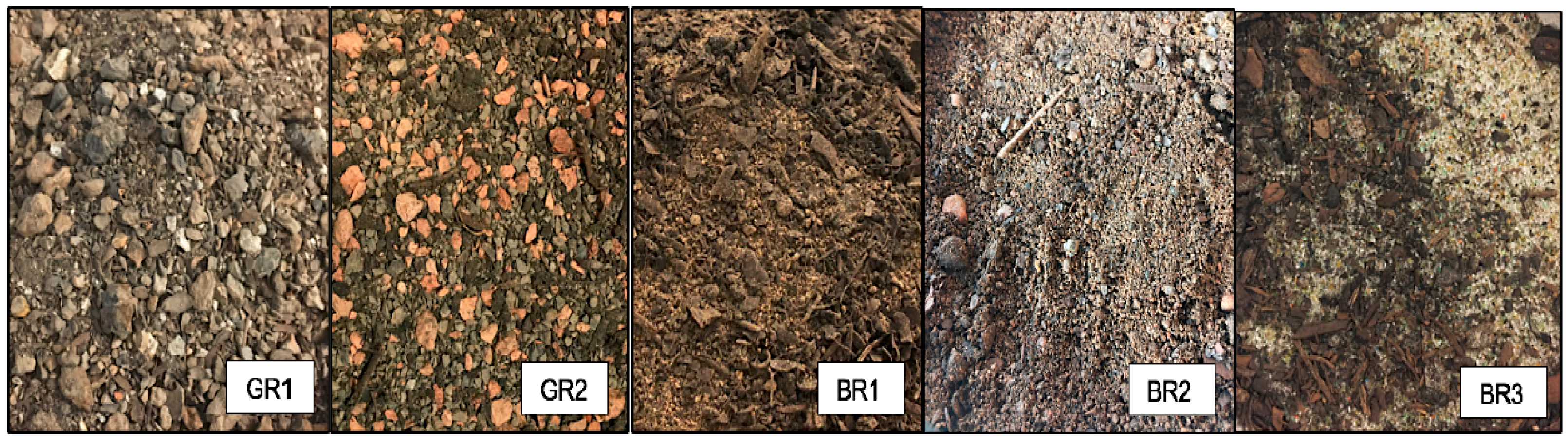
The LID media used in this research were sourced from local suppliers. The two green roof substrates were provided by LiveRoof Ontario and Gro-Bark. Gro-Bark also provided two bioretention substrates, one of which contained glass sand. The third bioretention substrate was provided by EarthCo Soil Mixtures. Overall, two green roof media (GR1, GR2) and three bioretention media (BR1, BR2, BR3) were used in experimental testing and numerical modelling. The five substrates are shown in
Figure 1. Visual inspection indicated that, the green roof materials were coarser in comparison to the bioretention materials. The bioretention materials have a more uniform appearance with sand and wood chips being the most distinct constituents.
Table 1 shows the measured organic content and specific gravity of the 5 substrates. The organic content was determined by placing the sample in a muffler oven set to 550 °C for approximately 2 h [
18,
20]. The amount of organics within the sample was determined by taking the difference in mass before and after the dry combustion. The addition of organic material acts as a lightweight component and is beneficial in decreasing the load on the green roof [
30]. Moreover, the organic material provides a large water storage volume [
31] and helps deliver nutrients for plant growth [
30].
Furthermore, it is noted that the addition of organic material also assists in the reduction of the soil density [
30]. As shown in
Table 1, the specific gravities of the green roof media are smaller compared to the bioretention media. The specific gravity was determined using the pycnometer method [
21].
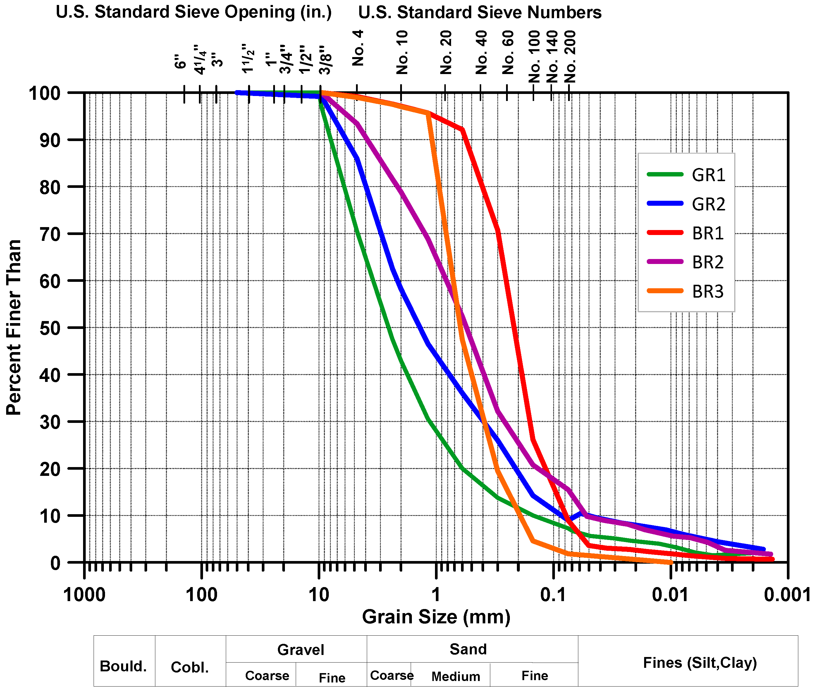
To determine the particle size distribution curve (PSD), the sieve test [
22] and hydrometer test [
23] were performed. The PSD of all five substrates is shown in
Figure 2. From the PSD, both green roof media contains a large percentage of gravel (>2 mm) in comparison to the bioretention media, which is consistent with the visual inspection done initially. The bioretention materials contain a large percentage of sand (0.05–2 mm), with BR3 having 97% sand. All the substrates analyzed were quite coarse and are expected to have high saturated hydraulic conductivity values leading to good drainage during flooding conditions.
3.2. Measured Hydraulic Properties
3.2.1. Saturated Hydraulic Conductivity
To determine the saturated hydraulic conductivity, the constant head test was performed. In order to successfully measure the saturated hydraulic conductivity for these very coarse substrates, preparation of the sample was the key. For this test, two side ports were installed into a compaction permeameter in order to attach the two open manometer tubes. The height of the compaction permeameter is 18.0 cm and the diameter is 15.2 cm. The distance between the two side ports is 7 cm.
Each LID media was then packed within the permeameter to the dry bulk density of 1 g/cm
3. A dry bulk density of 1 g/cm
3 was used as alternative studies have obtained sample cores from live sites and used a dry bulk density of approximately 1 g/cm
3 [
15,
18,
32,
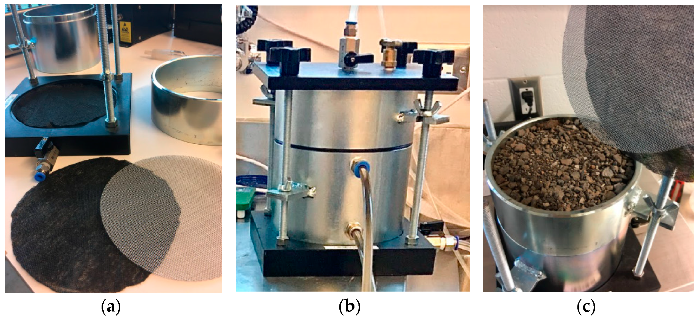
33]. The oven dried sample was split using a splitter into four different bowls to help reduce the sample bias. To reduce particle segregation, water was added so that the sample reached a gravimetric water content of 2%. A packing procedure was adopted to avoid horizontal layering. When packing, the first lift was poured in and gently compacted. The top of the layer was then lightly scraped before pouring in the next lift to avoid horizontal layering of the sample. Once the permeameter was filled, the geotextile and metal mesh were placed at the top and then were sealed with an appropriate cover (
Figure 3c).
Carbon dioxide was passed though the permeameter to assist in flushing out the air. Once the sample has been flushed with CO2, the permeameter was attached to a water reservoir and two manometers. In order to reduce air entrapment in the system, de-aired water was used. The saturated hydraulic conductivity was determined by measuring the volumetric flowrate by maintaining a constant head.
3.2.2. Measurement of SWCC
A popular method to measure the SWCC is the simplified evaporation method [
19]. To measure the SWCC, the HYPROP measurement system [
34] which employs the evaporation method was used.
With the exception of the packing procedure, the measurements were made following the procedure as described by the manufacture [
34]. For sample packing, a procedure similar to the one described for the hydraulic conductivity measurements was used. The sample was packed in three lifts. In order to reduce particle segregation during packing, the sample was wetted to a water content of 2%. The first lift is poured into the silver sample ring that is provided with the HYPROP equipment. The sample is compacted with 10 blows using a round shear box extruder and the side of the sample ring is tapped 5 times. The top of the layer was lightly scraped to avoid horizontal layering. Following a similar procedure, the second lift is poured into the sample ring. For the third lift, the excess sample at the top of the sample ring is scraped off with a straight edge (
Figure 4a).
3.3. Pedotransfer Function
In total, 19 different pedotransfer functions were considered for each of the LID substrates. Regression models, physicoempirical models, and the use of an artificial neural network utility were the three types of PTFs that were used to predict the SWCC.
Guber and Pachepsky [
35] have developed a computer program, named CalcPTF, that utilizes regression equations to predict the unsaturated hydraulic properties from routinely measured soil properties. Routinely measured soil properties include the percentage of sand, silt and clay, the organic content and the dry bulk density. CalcPTF contains numerous PTFs, where some estimate the Brooks and Corey [
28] parameters and the others estimate the van Genuchten [
27] parameters.
Table 2 provides the details of the soil inputs required for the various PTF in CalcPTF.
The physicoempirical models utilize the particle size distribution to predict the SWCC as they are based on the similarity of shape. The two physicoempirical models selected to be analyzed for this research are the Arya and Paris [
48] model and the Modified Kovacs Model developed by Aubertin et al. [
49].
Arya and Paris [
48] presented one of the first physicoempirical model and is especially preferred in practice as it works well with various soil types [
7,
50]. The Arya-Paris (AP) model divides the particle size distribution curve into fractions, where the larger particle sizes relate to a larger soil water content. The AP model estimates the volumetric water content by estimating the pore volume and determines the soil pressure by converting pore radii using the capillary theory [
48].
The other physicoempirical model analyzed is the Modified Kovacs (MK) Model [
49]. This model has been shown to work well with tailing materials, granular and cohesive soils [
50]. As the LID material is highly granular, it was of interest to see if this model would work well for LID materials. The major difference between the MK model and the AP model is that the MK model only uses the coefficient of uniformity (Cu) from the particle size distribution, rather than directly using all of the points measured in the PSD.
The third PTF type analyzed uses neural network predictions. Rosetta Lite DLL (Dynamically Linked Library) is included within the HYDRUS software [
25] to help predict the van Genuchten [
27] parameters and saturated hydraulic conductivity [
9]. Rosetta’s predictive capabilities rely on textural class, textural distribution, bulk density, and one or two water retention points as inputs. While the inclusion of additional input data generally leads to improved accuracy, soil information may be limited in some cases. In such scenarios, Rosetta adopts a hierarchical approach to estimate SWCC and
Ks values, using either a limited or more extensive set of input data. This approach is reflected in the five available models, each calibrated on the same dataset. The simplest model uses a lookup table to provide average hydraulic parameters for each soil textural class (e.g., sand, silty load, clay loam). In contrast, the other four models rely on neural network analysis [
9] and employ additional input information such as the percentage of sand, silt, and clay (SSC), dry bulk density (BD), and the water content at 33 kPa and 1500 kPa suction values. By incorporating this hierarchical approach, Rosetta can make accurate predictions with limited input data, while also allowing for more detailed predictions when additional information is available.
3.4. Statistical Analysis
The measured and predicted SWCC are compared using statistical analyses and visual inspection. To confirm the validity of the statistical analysis, a visual inspection of the predicted to the measured data is recommended by Schunn and Wallach [
51], as they can provide non-overlapping information. The coefficient of determination (
R2) is a statistical measure to assess how well the trend in the predicted data matches the measured data. Obtaining a
R2 of 1 refers to 100% of the predicted data matches the trend of the measured data. Nevertheless, a
R2 of 1 does not necessarily mean the predicted data matches the measured data. Thus, to determine the deviation from the actual value of the measured data, both the mean square deviation (MSD) and the mean absolute deviation (MAD) are estimated. Lower MSD and MAD values indicate less deviation between the predicted and the measured values. The
R2, MSD and MAD are calculated as follows:
where
n is the number of data points,
θm and
θp are the measured and predicted volumetric water content, respectively. The difference between the
MSD and
MAD measure of goodness-of-fit is that the
MSD squares the deviation, thus placing emphasis on points that do not fit the measure data well in comparison to points that do fit well. The
MAD estimation is a more simplistic approach that puts equal weight on all deviations and is therefore suitable for relatively noise-free data. A
MAD estimation of 3 represents that, on average, each value is off by 3 from the mean, thus presenting a more direct measure of the data.
3.5. Numerical Analysis
The impact of measured versus predicted hydraulic properties on the performance prediction of LID systems was assessed using HYDRUS 1D software [
25]. HYDRUS is a modelling software used in the analysis of water flow and solute transport in variably saturated soils. Various studies have demonstrated that HYDRUS provides good accuracy in predicting the hydraulic response of different LID systems [
8,
15,
52,
53,
54]. In order to set-up the numerical model, the material properties, climate data, geometry, initial conditions and boundary conditions are required. The material properties used for the analysis are the measured soil properties and the predicted van Genuchten [
27] parameters from the PTFs.
The models for the bioretention media were simulated with a 100 cm deep soil profile overlaying 300 cm of loamy sand. A 15 cm soil profile was simulated for the green roof substrates, which corresponds to an extensive green roof [
55]. The lower boundary condition of the models was set to free drainage. The upper boundary condition was set to atmospheric boundary condition with a surface layer, where the green roof substrate was restricted to 0 cm of surface head. Thirty years of daily records of precipitation and potential evaporation values for Toronto, Canada constituted the atmospheric boundary.
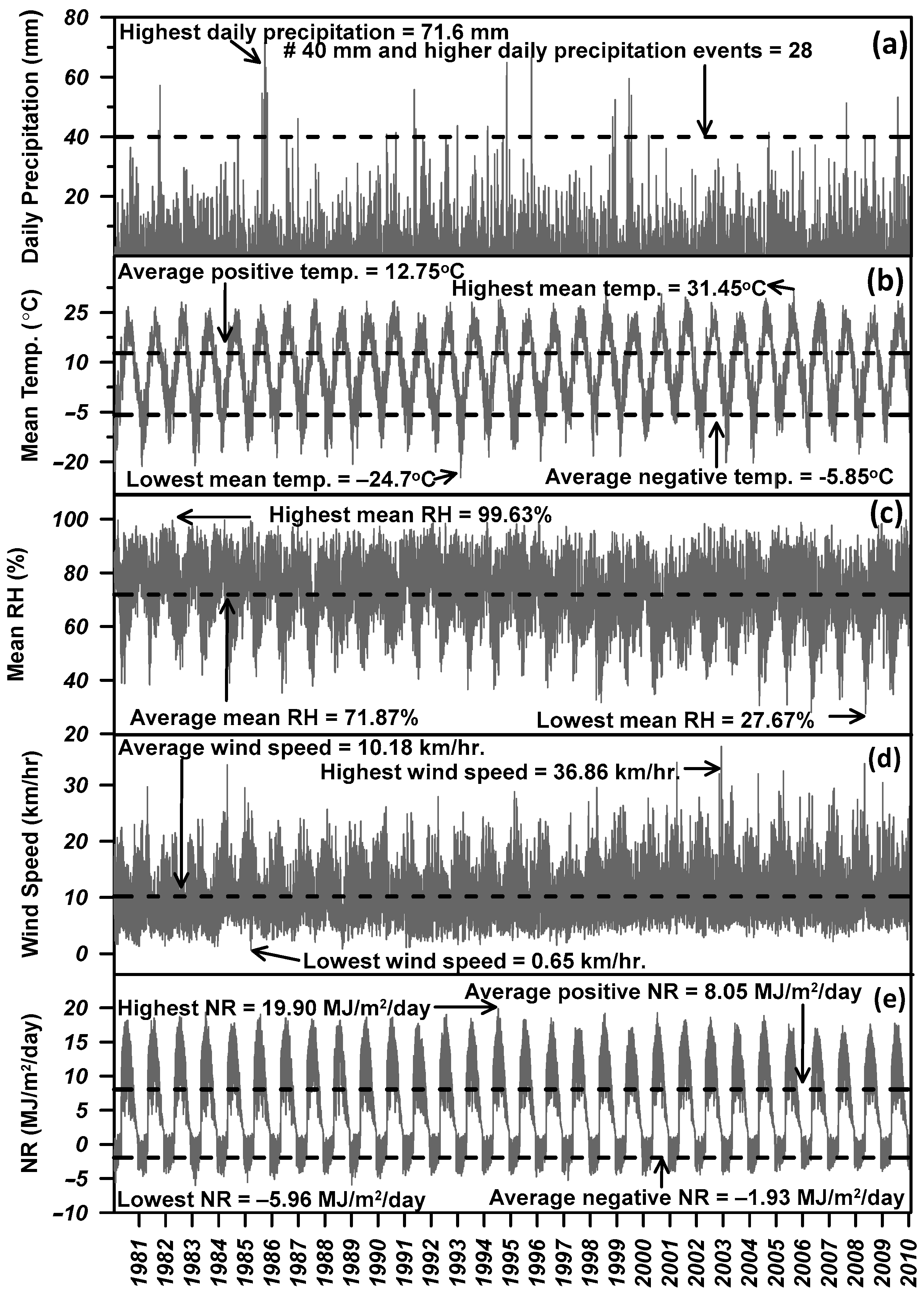
Toronto historical climate data between 1981 to 2010 was collected from Environment and Climate Change Canada portal [
56]. The dataset comprises of the daily values of precipitation, relative humidity, temperature, wind speed, and net radiation (
Figure 5). The compiled climate datasets were statistically analyzed to compute historical averages, maximum and minimum values, and other pertinent information for various climate variables over the 30 years [
57,
58,
59]. In order to estimate the potential evaporation, Penman [
60] method was used. In total, 8250 active days were modelled, where the active period represents the time when the ground is thawed thus allowing water to infiltrate into the soil. The concept of active days has been introduced by Fredlund et al. [
50] and has been used in various studies [
58,
61,
62].
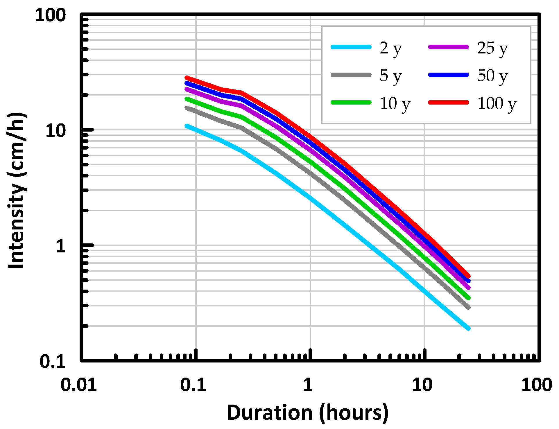
For extreme precipitation events, historical intensity-duration-frequency (IDF) curves were collected from Environment and Climate Change Canada [
63].
Figure 6 presents the IDF curves for Toronto. For this study, the 48-h storm duration was used as it provides meaningful analysis of a greater quantity of water entering the LID system compared to the other storm durations. With the acquired IDF data, synthetic design storms were developed using the method proposed by Kiefer and Chu [
64], also known as the Chicago design storm.
The allowable ponding was taken as zero for the green roof. On the other hand, bioretention facilities are designed for ponded conditions as they cater to a greater catchment area in addition to precipitation that directly infiltrates the system. According to Credit Valley Conservation and Toronto and Region Conservation Authority [
55], the maximum ponding depth should be between 15–25 cm. Therefore, the allowable surface ponding was set to 20 cm in the models that were representative of bioretention facilities.
The amount of stormwater runoff is dependent on the catchment area and degree of imperviousness of the area for the bioretention system [
65]. A ratio known as the Impervious to Pervious ratio (
I/P) combines these two factors in the following relationship:
where
Vi is the volume of the influent,
d is the precipitation depth, and
AB is the area of the bioretention system. As HYDRUS 1D treats additional precipitation in units of depth rather than volume, the equation can be rewritten as follows [
66]:
where
di is the depth of the influent. If the percentage of the catchment area was 10% and the percentage of impervious area was 60%, the
I/P ratio would be 6. This would result in a depth of influent 7 times greater than the precipitation depth. It is suggested that the bioretention system should have an
I/P ratio of 5 to 20 [
55]. An
I/P ratio of 6 is used for this research for the bioretention systems. For the green roof system, there is no additional stormwater entering the system other than the precipitation directly entering the system. Therefore, the green roof system would have an
I/P ratio of 0.
An initial condition of −100 cm of head was assumed for the modeling domain. As the simulations were carried out using thirty years of climate data, the initial conditions do not greatly impact the overall results over the long term. Running the thirty years of data, then applying the final conditions as the new initial conditions did not impact the overall results from the numerical simulations. On the other hand, incipient soil moisture conditions at the start of the storm could play a significant part in design storm analysis. A substrate with wet initial conditions would lead to a greater runoff or ponding depth in comparison to drier initial conditions. Daily soil water saturation data from the 30-year Toronto historic climate data simulation was analyzed in detail and average soil pressure conditions corresponding to 50th percentile saturation was extracted as the initial conditions for the design storm simulations.
4. Experimental Results & PDF Estimations
4.1. Hydraulic Properties
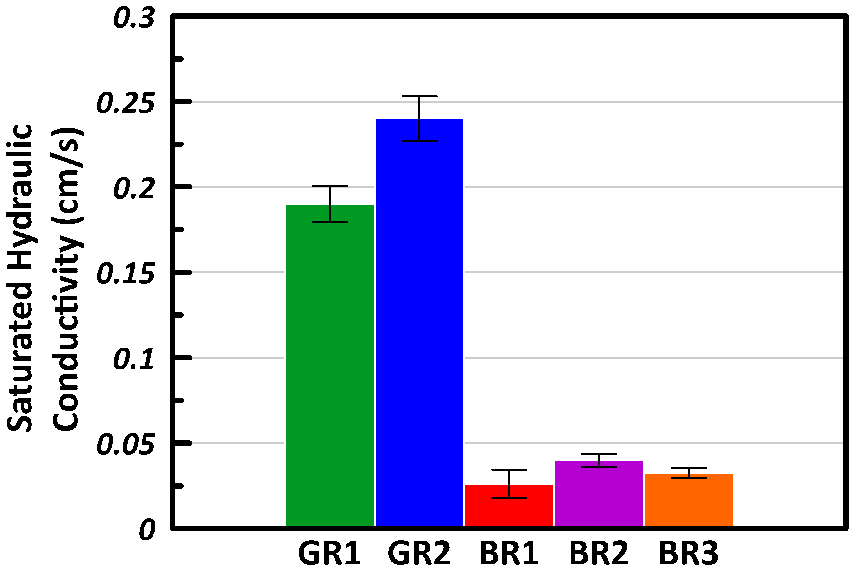
Averaged saturated hydraulic conductivities (
Ks) for the five LID media as well as the error bars are shown in
Figure 7. Overall, the
Ks measured for the green roof materials is one order of magnitude higher than the bioretention materials. These results are consistent with the PSD, which indicated that the green roof materials are coarser compared to the bioretention materials.
GR1 has a greater percentage of gravel in comparison to GR2, resulting in slightly higher
Ks due to the increased void space assisting the water mobility. On the other hand, the bioretention media is designed to undergo ponding and assist in the reduction of storm water pollutants in addition to flood prevention. Thus, to capture the contaminants whether through sorption, volatilization, or filtration, a lower
Ks in comparison to the green roof media is preferred [
67].
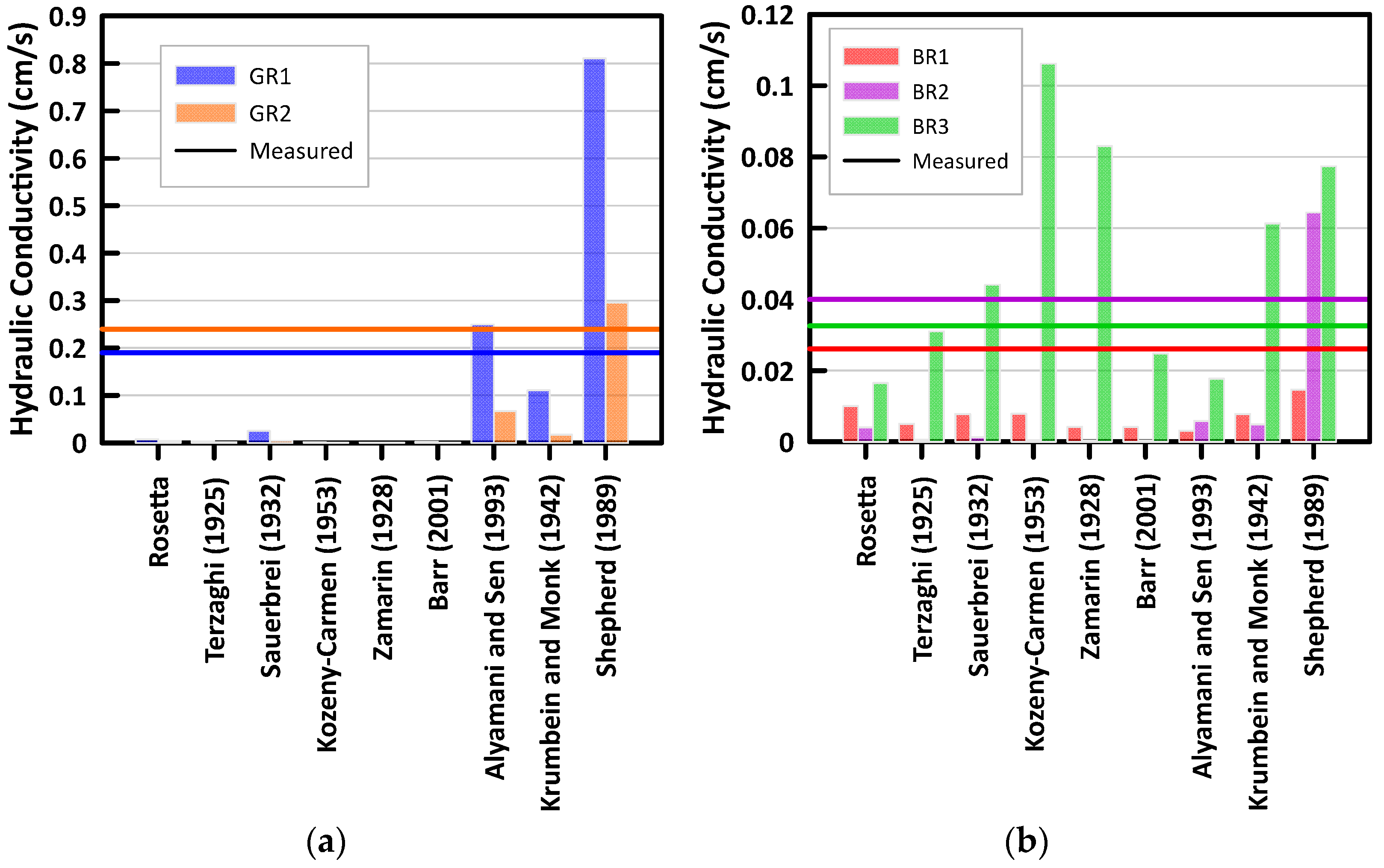
Predictions for Hydraulic Conductivity
Pedotransfer functions are also used to estimate saturated hydraulic conductivity. Rosetta provides estimates for
Ks in addition to estimates for water retention. Devlin [
68] has developed a program, called HydrogeoSieveXL, to estimate
Ks from grain-size distributions curves using 15 different methods.
Figure 8 presents the estimated
Ks from Rosetta and eight methods [
69,
70,
71,
72,
73,
74,
75,
76] included in the program by Devlin [
68]. Some methods included within HydrogeoSieveXL were excluded as the material failed the criteria required for that
Ks estimation model.
Overall, both Rosetta and the methods found in HydrogeoSieveXL underestimate the measured Ks for the LID materials considered in this study. In general, the methods underestimate Ks values for the green roof substrates by a magnitude of two and the bioretention materials by a magnitude of one. BR3 obtained the closest estimates, demonstrating that uniform-graded materials perform best when estimating using physicoempirical methods.
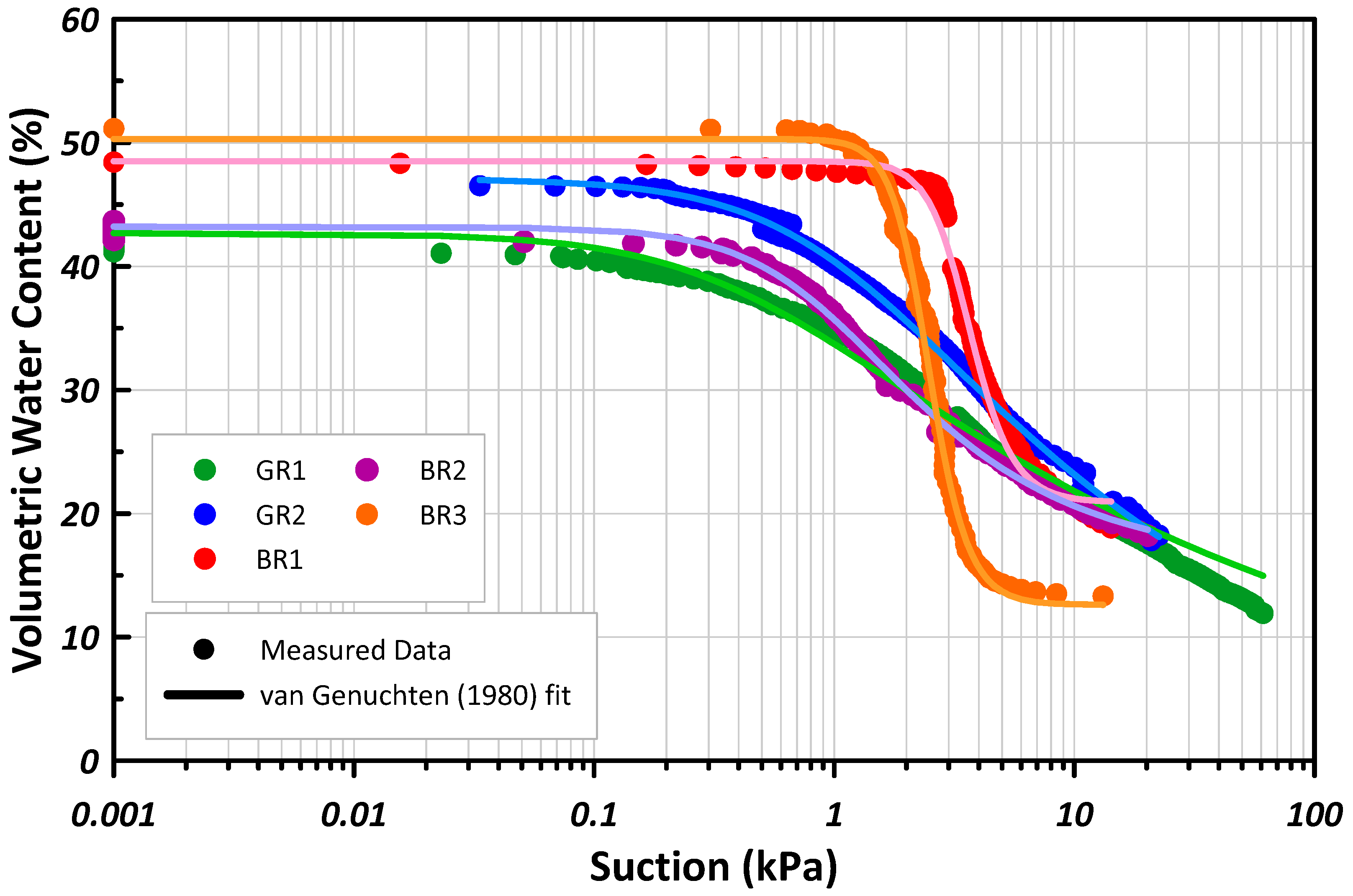
4.2. SWCC Experimental Results
The SWCC for the five LID materials were measured and are illustrated in
Figure 9.
Figure 9 also demonstrates how good the fit is between the experimental values and fitted curved using van Genuchten [
27] equation. The fitted van Genuchten [
27] parameters to the measured SWCC data are presented in
Table 3.
The air entry value (AEV) is the suction value at which air first enters the saturated soil resulting in the start of desaturation. From
Figure 9, it can be observed that BR1 and BR3 have a larger AEV compared to the other substrates. From
Table 3, the
α parameter in the van Genuchten [
27] equation is approximately equal to the inverse of the AEV. The
α parameter is smaller for the bioretention materials in comparison to the green roof materials, with the exception of BR2.
The
n parameter presented in
Table 3 correlates with the pore size distribution. A high
n value signifies a narrow pore size distribution, leading to a steeper SWCC as the water content drains over a narrow suction range. As observed in
Figure 9, both BR1 and BR3 have steep curves, thus a greater
n value. Note that BR1 and BR3 are also classified as poorly graded according to the soil classification using USCS. The green roof substrates have a smaller
n value which allows the system to retain water over a greater suction range. Both green roof substrates are classified as well-graded according to the USCS soil classification.
5. Performance Evaluation of PTFs for SWCC
To compare the performance of various PTFs to the measured SWCC, the
R2, MSD and MAD values were calculated.
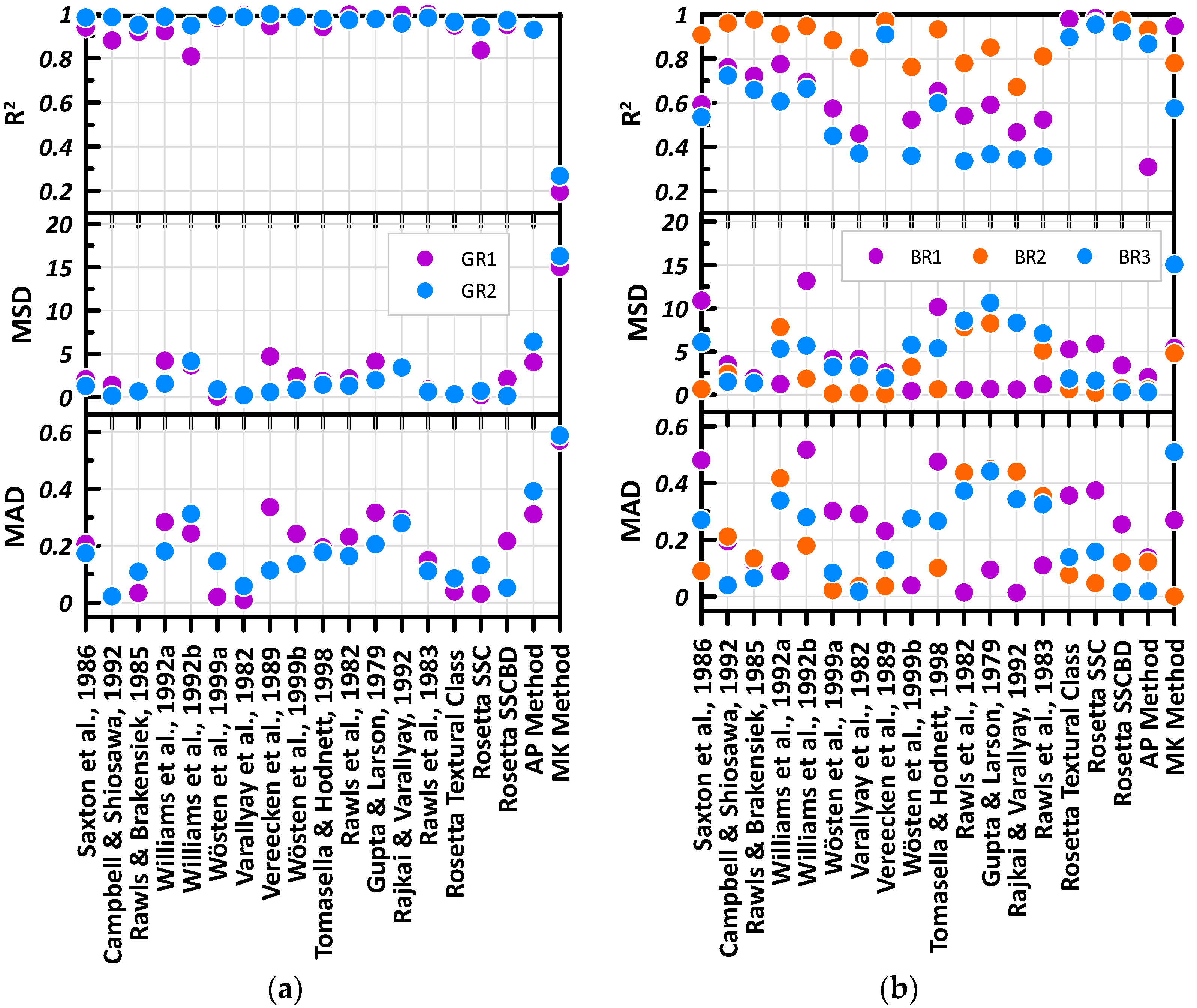
Figure 10 presents a scatterplot of the computed
R2, MSD, and MAD values for the green roof and bioretention substrates. From
Figure 10, it can be observed that the trend relative magnitudes are captured well for both green roof substrates in comparison to the bioretention substrates. On average, both of the green roof substrates (GR1 & GR2) have an
R2 value greater than 0.90, with the exception to the MK method that had an
R2 value less than 0.30. Whereas the bioretention substrates have low
R2 values, in some cases reaching a low
R2 value of 0.30. In addition, there is a lower deviation observed between the measured and predicted SWCC for the green roof substrates in comparison to the bioretention substrates. The MSD value for the green roof substrates generally have a value less than 4, with an average of 1.8 without the MK method. Whereas the bioretention substrates have MSD values exceeding 10, with an average of 3.9. The MAD estimation, as stated earlier, presents a more direct measure of the data where a value of 0.5 means that the volumetric water content of the predicted model is, on average, off by 0.5 from the mean of the measured data. As shown in
Figure 10, the bioretention substrates presents a larger deviation in MAD and MSD values compared to the green roof substrates. A visual examination is required to assess where the predictions are most problematic.
After examining the statistical analysis of the predicted to the measured SWCC, it can be concluded that some of the PTF methods work better for certain substrates compared to the others. In general, the PTFs from the CalcPTF program and from Rosetta performed better for the green roof materials considered for this research in comparison to the bioretention materials. On the other hand, the AP method performs relatively well for the bioretention materials. Overall, the MK model is observed to perform poorly for all substrates considered in this research. Upon closer investigation, it can be concluded that CalcPTF and Rosetta show poor performance for materials that contain the larger percentage of sand. This leads one to the conclude that, for the most part, PTFs performance is largely dependent on the percentage of the certain particle sizes. Nevertheless, it is important also to note that both the CalcPTF program and Rosetta do not take into consideration the percentage of gravel within the substrate.
5.1. Validity of the Statistical Analysis through Visual Examination
Visual inspection of the measured and predicted SWCCs was carried out to determine which core features of the SWCC is not predicted well. The core features of the SWCC include the saturated and residual water contents, air entry value, and pore size distribution.
Figure 11 presents the five substrates and compares the measured versus predicted SWCC for four different PTFs. As there is a large number of estimations that were considered from the CalcPTF program, the PTFs that provided the best comparison from a statistical perspective are presented in
Figure 11. The selected PTFs from the CalcPTF program produced an
R2 value closer to 1 and a lower MSD and MAD value.
From
Figure 11, it can be observed that the predicted curves capture the slope of the measured SWCC fairly well. The predicted curves for BR2, GR1 and GR2 follow a gradual sloped curved, with some exceptions such as the MK method. Whereas the measured SWCCs for BR1 and BR3 have steep SWCCs which is indicative of the fact these materials drain over a narrow suction range compared to the other measured SWCCs. The predicted curves for BR1 and BR3 present a steep SWCC, similar to the measured SWCCs. Thus, the slopes of the predicted curves presents a good fit to the measured curves. The AEV of the predicted SWCCs rarely overlap with the measured AEV, as shown in
Figure 11. Predicted curves that underestimate the AEV present a relatively better fit compared to the predicted curves that overestimate the AEV. For example, the AP method presented in
Figure 11c for BR1 overestimates the AEV, leading to an extremely poor fit. Choosing a PTF that overestimates the AEV wrongfully estimates the substrate’s ability to stay completely saturated over a greater suction period and would result in erroneous designs.
Most of the predicted SWCCs overestimate the saturated water content, some by as much as 10%, which implies that the storage of the substrate is greater than expected. There are some PTFs that use the particle density and dry bulk density to estimate the porosity. This porosity value is then assumed to be equal to the saturated volumetric water content. This tends to overestimate the saturated volumetric water content as shown in
Figure 11. However, it should also be noted that it is somewhat difficult to achieve complete saturation during the experimental measurements. This is even after leaving the substrate core in a water bath for 24 h. It is possible that when transferring the substrate core from the water bath to the HYPROP apparatus, gravitational drainage occurs thus emptying the macropores within the porous substrate or the sample never gets completely saturated due to the air entrapment. Currently, there are no mechanisms available in the equipment to ensure no air entrapment. It should be noted that even if another measurement method, such as pressure plate extractor, is to be employed and a complete saturation via vacuum or carbon dioxide flush is to be attained, complete saturation in field condition is never possible. Therefore, it can be argued that attainment of complete saturation under laboratory conditions is perhaps not the best representation of field conditions and overestimation by PTF can potentially grossly overestimate the total available storage in LID systems.
5.2. Numerical Modelling Results
The water balance at the ground surface describes the amount of water that moves across the soil-atmosphere boundary. Through the assessment of a water balance, relevant components such as water storage capacity, infiltration or drainage can be quantified. This assists in the analysis and design of the substrates performance when used in LID applications. Components of the water balance at the ground surface include precipitation (
P), potential evaporation (
PE), actual evaporation (
AE), transpiration (
T), surface run-off (
RO), and net infiltration (
NI). The
NI refers to the amount of water that enters the soil surface overcoming the evaporation and surface runoff. It can be described as:
The AE is also dependent on prevailing water quantity in the near surface soil layer and is therefore always less than the PE, if the surface does not remain saturated. HYDRUS estimates AE by using a system-dependent atmospheric boundary condition at the top of the modeling domain. The potential flux is dependent on external conditions, such as precipitation and evaporation, while the actual flux depends on the external conditions as well as the transient soil moisture conditions.
As shown in Equation (8), if the actual evaporation is high, the NI decreases accordingly. Higher precipitation intensities might result in exceeding the infiltration capacity of the soil resulting in surface run-off, thus decreasing the NI. Generally, a higher soil water retention and low saturated hydraulic conductivity (Ks) tends to increase the AE, thus decreasing NI. A lower Ks and higher air entry value implies that it would take longer for water to move deeper into the soil, thereby allowing evaporation to occur as the water remains near the surface.
5.2.1. Long-Term Analysis
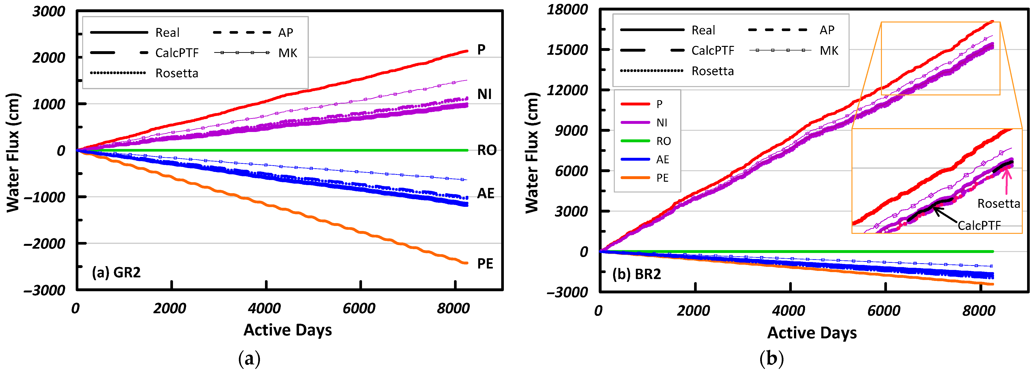
The HYDRUS 1D software was used to evaluate the performance of the hydraulic properties from PTFs to the measured hydraulic properties using thirty years of Toronto’s historical climate data. The water balance at the ground surface using the measured and predicted soil hydraulic parameters is presented in
Figure 12 for GR2 and BR2. Note that the water exiting the system is assumed to be negative while the water entering the system is considered positive.
Table 4 contains the van Genuchten [
27] parameters used in the numerical simulations for GR2 and BR2′s water balances. As there were many regression equations contained within CalcPTF, the equation that produced a better comparison from a statistical perspective (high
R2, low MSD and MAD) was chosen. Additionally, no surface runoff was observed for any of the substrates as they have a high saturated hydraulic conductivity.
From
Figure 12a, it can be observed that the PTFs overestimate the
NI for green roof material. The difference in
NI calculated from measured and estimated (MK method) hydraulic properties is 500 cm at the end of the 30-year period. This comes out to be 167 mm every year on average. This is consistent with the statistical analysis for GR2, where the MK model performs poorly in comparison to CalcPTF. The difference between CalcPTF and the measured hydraulic properties for
NI is 50 cm, which is quite small in comparison. The greater
NI results in a greater bottom flux (
BF) leading to overdesign for a green roof. The
BF describes the outflow at the bottom of the substrate as free drainage was assumed at the bottom boundary. During a storm event, it is ideal to mitigate the water travelling out of the green roof. As reducing peak flow during storm events is a key design criterion for LIDs, a decreased
BF for green roofs is preferred.
Figure 12b presents the water balance for BR2. The water balance of the predicted and measured hydraulic properties presents somewhat similar results. Whereas the PTFs overestimated the
NI for GR2, the PTFs for BR2 underestimate the
NI, with the exception of the MK model. CalcPTF has the closest results to the measured simulation, with a
NI difference of 165 cm at the end of the 30-year simulation. The MK model performs poorly compared to the other models, with a
NI difference of 587 cm from the measured. The performance of the PTFs is consistent with their ability to predict hydraulic properties. Similar observations were made for BR1 and BR3, where simulations using predicted and measured hydraulic properties resulted in relatively close
NI values. Therefore, it can be concluded that the
NI estimates are less sensitive to soil hydraulic properties for LID systems that accept a large quantity of water.
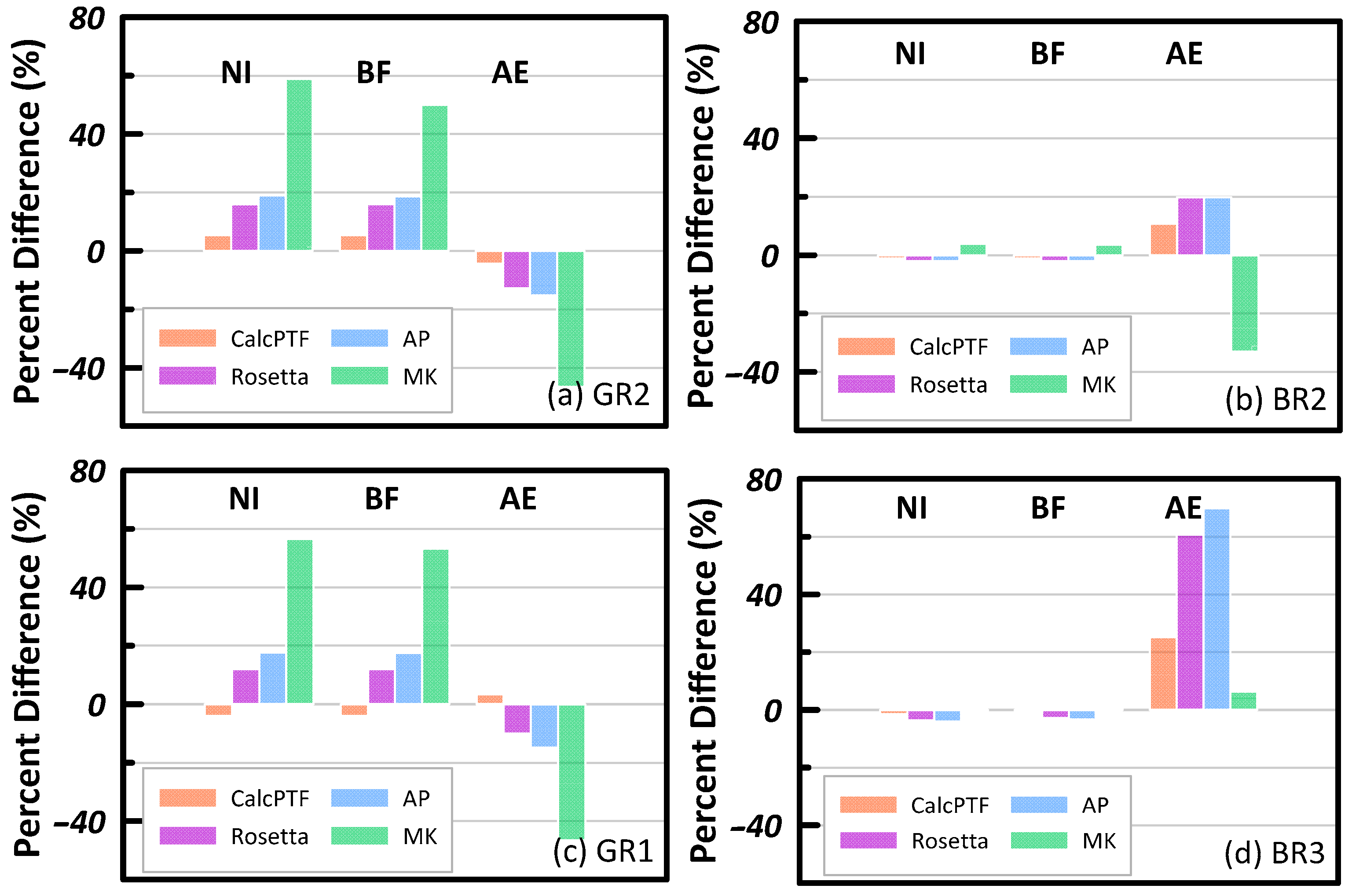
To further analyze the water balance results, the percent difference for each PTF and the cumulative
NI,
AE, and
BF are examined and shown in
Figure 13. The cumulative values for
NI,
AE, and
BF using the measured soil hydraulic properties are used as the baseline. It is evident that there is a greater percent difference between the
NI and
BF for the green roof substrates whereas the bioretention substrates have a small, almost negligent, percent difference. This further demonstrates that the effects of the soil hydraulic properties get muted when large quantities of water enter the system. There is also a great percent difference in
AE for the bioretention that is not as noticeable in the water balance shown in
Figure 12b.
5.2.2. Extreme Precipitation Analysis
The performance of the PTFs to the measured hydraulic properties under extreme precipitation events was also evaluated using HYDRUS 1D. Design aspects of green roof and bioretention systems were evaluated using the measured and predicted hydraulic properties.
Green roofs assist in reducing the peak flow of a storm when compared to a conventional roof [
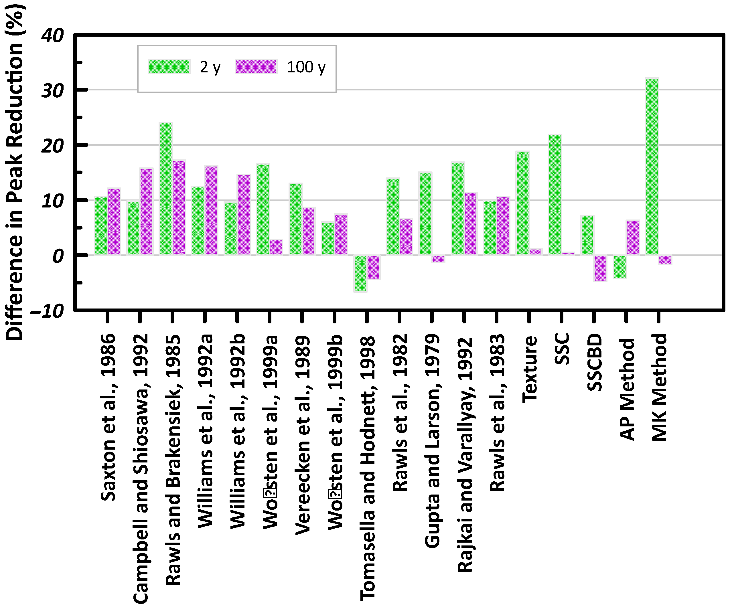
77]. The peak reduction can be determined by taking the percent difference between the peak of the storm event and the peak of the runoff.
Figure 14 presents the difference between the peak reduction using the measured and predicted hydraulic properties. A positive value implies that the measured hydraulic property has a greater peak reduction compared to the peak reduction obtained using the predicted hydraulic property. For example, the peak reduction for a 2-year storm using the measured hydraulic property and PTF developed by Campbell and Shiosawa [
37] results in a 91% and 81% reduction, respectively. Thus, the difference of 10% presented in
Figure 14 implies that a smaller peak reduction is predicted using this PTF. Overall, it is observed that smaller peak reductions are predicted when using PTFs, leading to overdesign of the green roof.
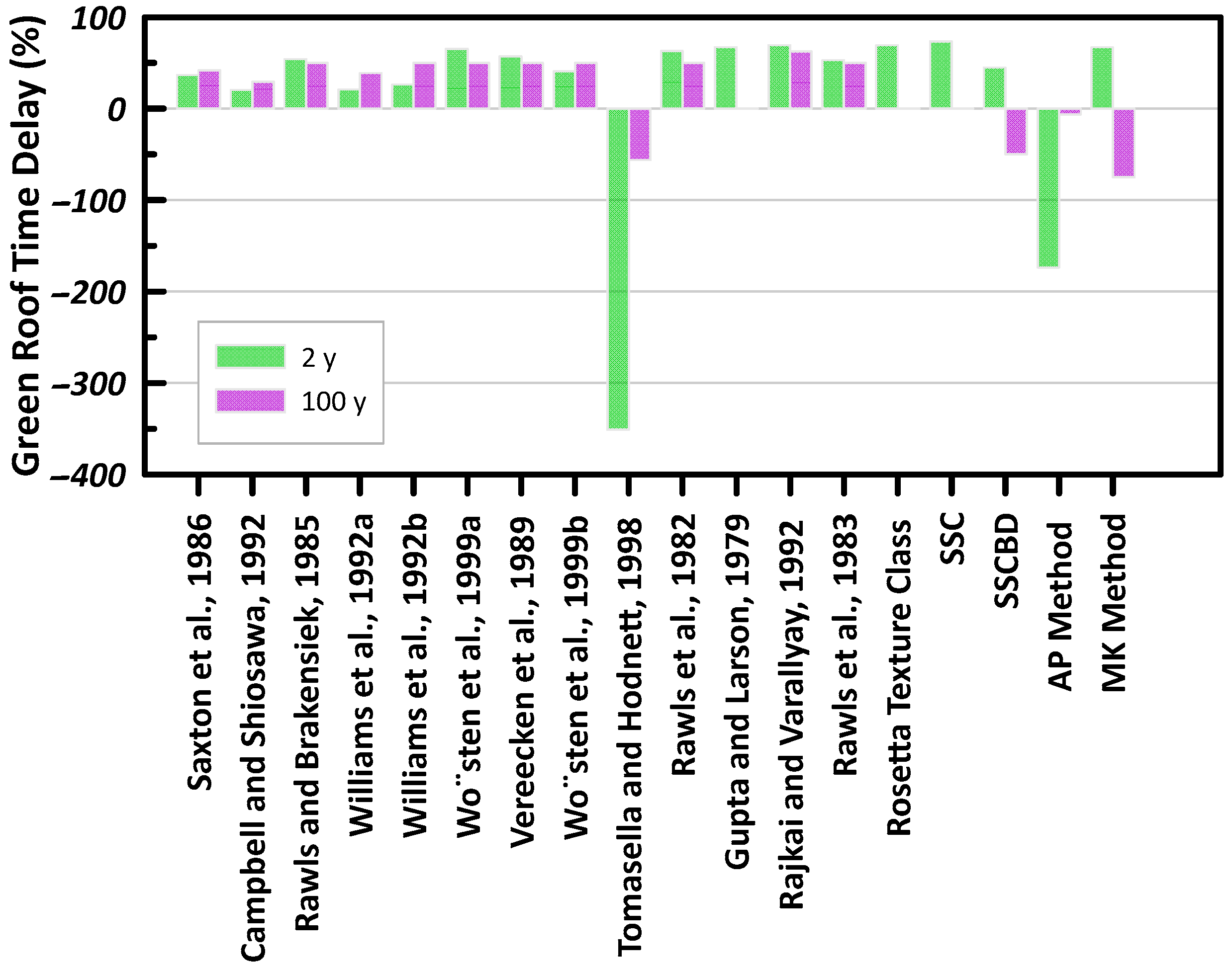
The peak time delay is significant in delaying the stormwater runoff quantity during a storm event. The time delay was determined by subtracting the time of the peak runoff from the peak of the storm event.
Figure 15 presents the percent difference of the time delay using the measured and predicted hydraulic properties. For example, using the measured hydraulic properties for a 100-year storm results in a time delay of 1.6 min. Whereas the predicted method developed by Rajkai and Varallyay [
46] resulted in a time delay of 0.6 min. The percent difference of 63% is presented in
Figure 15. As presented in
Figure 15, the percent difference between the measured hydraulic properties and predicted can range from 30% to 350%, with a majority resulting in a percent difference of 50%. This demonstrates that a large error is presented when using predicted hydraulic properties rather than measured.
A key design aspect for bioretention facilities includes the ability to allow for surface ponding. This assists in storing and treating stormwater runoff from large catchment areas. A maximum surface head of 20 cm was defined in the model in accordance with the maximum surface ponding defined by CVC and TRCA [
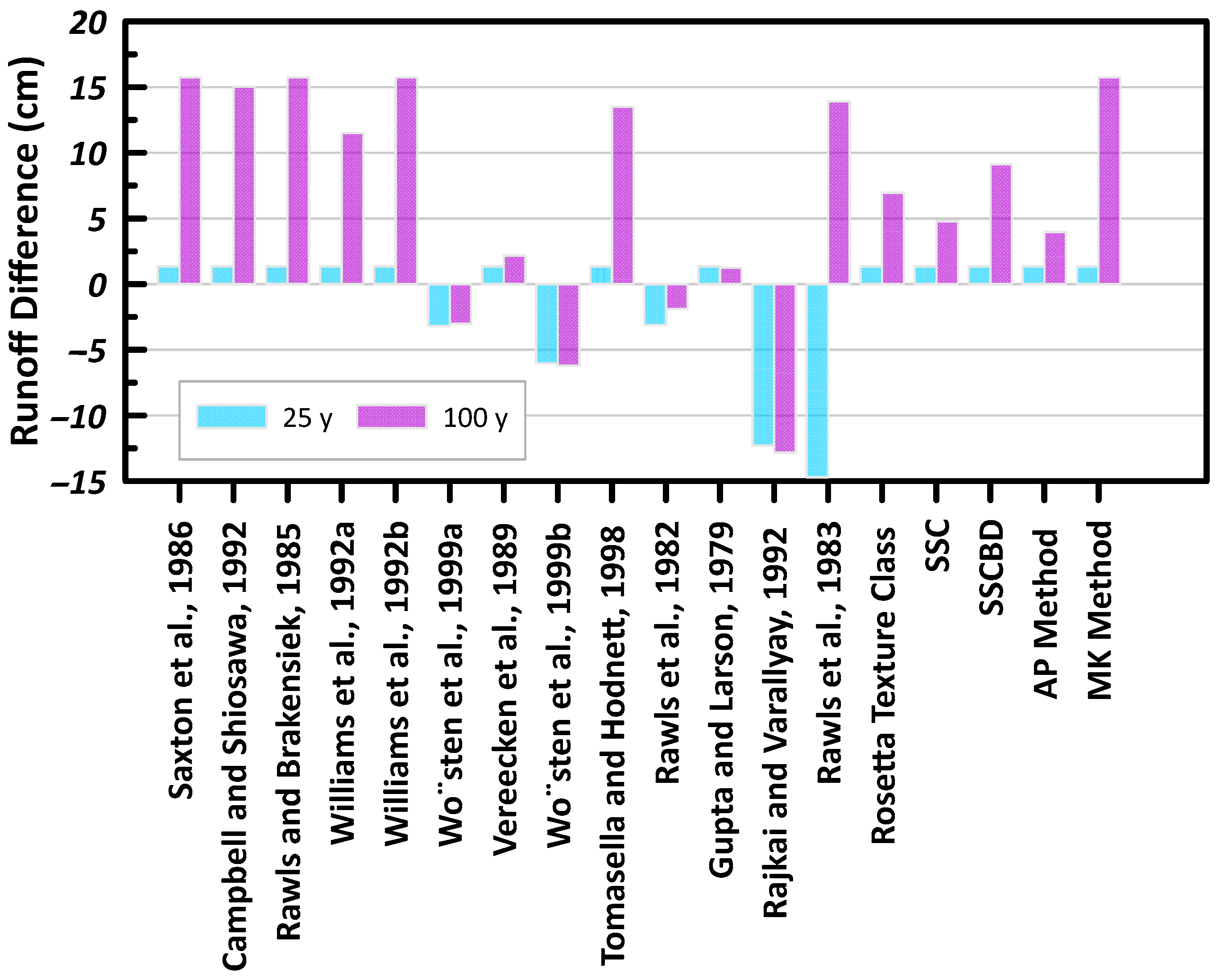
55]. A majority of the PTFs under the 25-year and 100-year storms surpassed the 20 cm maximum surface head. Therefore, the stormwater runoff from the bioretention facility is examined.
Figure 16 presents the stormwater runoff difference between the measured and predicted soil hydraulic properties. For example, the total amount of runoff simulated using the measured hydraulic properties and AP method for the 100-year storm event is 15.7 cm and 11.7 cm, respectively. Thus, the difference of 4 cm is presented in
Figure 16. The predicted methods from Saxton et al. [
36], Rawks and Brakensiek [
38], Williams et al. (b) [
39] and the MK method presented the greatest runoff difference of 15.7 cm for the 100-year storm event as they simulated no runoff. Thus, for a single 100-year storm, the difference in total runoff between the measured and predicted soil hydraulic properties can be as much as 15 cm. With increasing storm quantity, there is a greater variability presented in the predicted models.
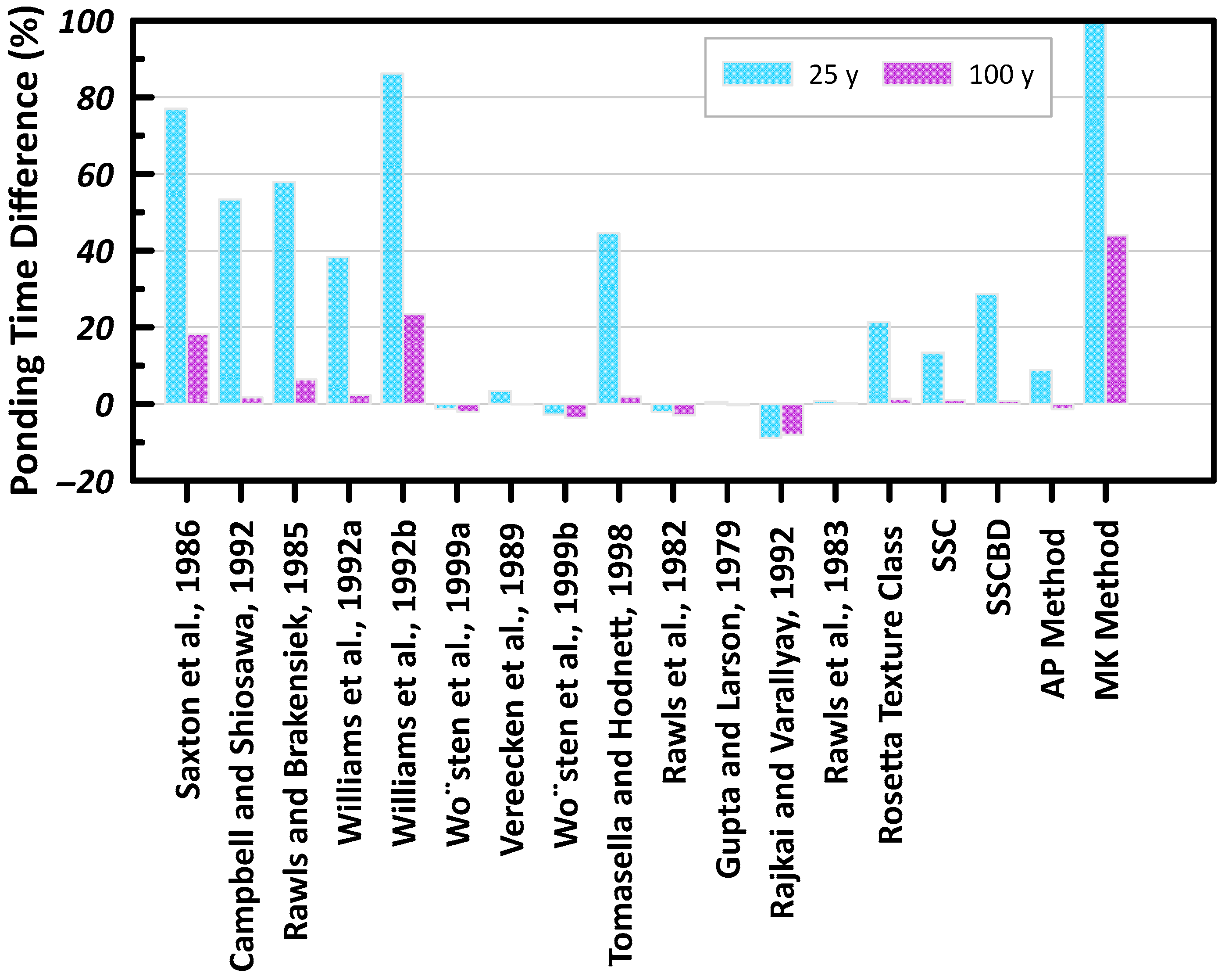
Figure 17 presents the ponding time percent difference between the measured and predicted soil hydraulic properties. For instance, the total ponding time for a 25-year storm using the measured hydraulic property and the AP model are 4.34 h and 3.96 h, respectively. The percent difference of 8.82 % is presented in
Figure 17. As the total ponding time for the 2-year storm event is almost negligible, examining the percent difference would result in a large, unrealistic value. It is noted that there is a greater percent different observed for the 25-year storm duration compared to the 100-year storm. With the increase in total storm quantity, there is an observed decrease in the percent difference in total ponding time between the measured and the predicted method. A majority of the percent difference between the measured and predicted method for the 100-year storms are less than 3%, with few exceptions.
According to CVC and TRCA [
55], it is recommended that the maximum allowable surface ponding time be 24 h after the storm event in order to avoid mosquito breeding sites. Thus, using the predicted soil hydraulic properties can result in large discrepancies between the ponding time using the measured soil hydraulic properties and the predicted. For example, the total surface ponding time for the 100-year storm duration using the measured soil hydraulic properties is 4.56 h. Using the MK method, the total ponding time for the 100-year storm is 2.55 h. Thus, a smaller surface ponding time is predicted leading to incorrect design of the bioretention facilities.
6. Concluding Remarks
Two green roof and three bioretention substrates were examined and characterized by measuring routinely measured soil properties. The samples for the green roof and bioretention materials obtained from different suppliers indicated that there is a wide variability in composition, geotechnical and hydraulic properties of these materials. Some highlights from these test results are noted as follows. The organic content of the LID substrates varied from 5.1% to 7.8%, with the bioretention media BR3 containing the greatest percentage. The specific gravity of the LID substrates varied from 2 to 2.8 g/cm3, with the green roof media having a smaller specific gravity compared to the bioretention. Most of the LID media have a specific gravity outside the typical range of soils, being 2.60 to 2.80 g/cm3. The green roof media had a greater percentage of gravel whereas the bioretention media had a greater percentage of sand. All of the LID substrates are quite coarse and are expected to provide good drainage during a storm event.
From the constant head test, the green roof substrates have a greater Ks compared to the bioretention substrates. As the bioretention systems are designed for ponded conditions, a smaller Ks, in comparison to the green roof media, allows for the contaminant capture. Finally, the SWCC was measured using the simplified evaporation method. The well-graded green roof substrates retained water over a greater suction range, whereas the poorly-graded bioretention substrates retained water over a narrow suction range. Measurement of unsaturated soil hydraulic properties for LID materials is costly, and time intensive leading to predictive methods such as pedotransfer functions. The use of these predictive methods for LID materials were examined in detail within this research.
Overall, there is a high level of uncertainty when using PTFs for LID materials. There is no one particular PTF model that works best for the all the LID materials that were considered. Furthermore, it was observed that the green roof substrates, GR1 and GR2, performed better using the PTFs from CalcPTF and Rosetta compared to the bioretention substrates, BR1, BR2, and BR3. As there is a large variability of the materials used in LID substrates, depending on the design criteria of the system, a PTF model that works well for one LID substrate may not work well for another. Historically, PTF models were designed by gathering a large quantity of measured soil data and creating a relationship. However, the soil data that is used to create the PTF models are typically natural soil and not the engineered soil used in LID systems. Thus, with the combination of the variability of materials used in each LID system and the PTF originally developed for native soil, there is no PTF model that can estimate all LID substrates.
The core features of the SWCC, including the air entry value, the saturated volumetric water content and the pore size distribution, were examined through visual analysis. For many of the examined substrates, the air entry value of the predicted SWCCs rarely matched the measured SWCC. Overestimating the AEV implies that the substrates is able to stay completely saturated under a greater suction value. This can lead to over estimation of AE and corresponding underestimation of quantity of water LIDs have to handle. Whereas the slopes of the predicted SWCCs generally had a good fit to the measured SWCCs. The PTFs were mostly able to predict whether the slope of the measured SWCC is steep or gradual. The saturated volumetric water content was overestimated for many of the examined substrates, sometimes as much as 10%. This would imply that the storage of the substrate is greater than expected as there is a greater saturated volumetric water content estimated.
In general, the PTFs have a limited capability to accurately estimate the SWCC of the engineered media. These substrates differ vastly when compared to natural, non-engineered soil as they are mixed to meet a specific design criterion. To examine the performance of the use of PTFs, long term simulations and extreme precipitation analysis using HYDRUS 1D was completed. Through numerical modelling, it was determined that measured soil hydraulic properties are more relevant for green roof systems in comparison to bioretention systems. This was observed by examining the percent difference of the measured cumulative net infiltration, actual evaporation and bottom flux to the predicted values. Using the AP method and Rosetta resulted in a percent increase of 15% in cumulative net infiltration for the green roof substrates. Using the MK method, a 60% increase in the cumulative net infiltration was observed for the green roof substrates. Whereas the bioretention media presented a small percent difference for all PTFs considered.
Similarly, key design criteria were examined for the green roof and bioretention under extreme precipitation events using the measured and predicted hydraulic properties. It was noted that the green roof design criteria, such as the peak reduction and peak time delay, varied vastly when using predicted hydraulic properties. The percent difference between the measured and predicted hydraulic properties for the green roof peak time delay can be as much as 300%. The bioretention design criteria, such as ponding, surface runoff, and ponding time presented large percent differences for the smaller storm durations. In some cases, the difference in surface runoff for the 25-year storm was as much as 14.7 cm and the 100-year storm as much as 15.7 cm. A percent difference of 100% is observed for the ponding time under 25-year storm durations and 40% for 100-year storm durations. This large discrepancy between the measured and predicted soil hydraulic properties can lead to unrealistic designs of the LID facilities. It is also highly recommended to conduct field experiments on the LID facilities to further examine their performance. This is especially important as it is well recognized that the substrates may be impacted by field procedures, such as compaction, which can lead to hydraulic properties that differ from those measured in laboratory settings. Therefore, field experiments would allow for a more comprehensive evaluation of the actual performance of the LID facilities and could help refine their design and construction to enhance their effectiveness.
As field and laboratory measurement of unsaturated hydraulic properties can be expensive and cumbersome, the use of PTFs can be seen as a great advantage. However, from a design perspective, accurate soil hydraulic properties are more important for systems that manage less water, such as green roof systems. Design performance criteria can differ vastly when using the predicted soil hydraulic properties compared to the measured leading to inaccurate designs of LID facilities under changing climate.
Author Contributions
Conceptualization, R.B.; methodology, R.B.; software, S.G.; validation, S.G. and R.B.; formal analysis, S.G.; investigation, S.G.; resources, R.B.; data curation, S.G.; writing—original draft preparation, S.G.; writing—review and editing, R.B.; visualization, S.G. and R.B.; supervision, R.B.; project administration, R.B.; funding acquisition, R.B. All authors have read and agreed to the published version of the manuscript.
Funding
This research was funded by individual Discovery Grant from Natural Sciences and Engineering Research Council Canada to Rashid Bashir.
Data Availability Statement
Data is available upon reasonable request to the corresponding author.
Acknowledgments
Thank you to LiveRoof Ontario, Gro-Bark, and Earthco Soil Mixtures for generously supplying the substrates used within this study. I would also like to thank Rashid Bashir for his continuous guidance and support and Kunjan Rupakheti for his advice in the laboratory.
Conflicts of Interest
The authors declare no conflict of interest.
References
- Juliá, F.E.; Snyder, V.A.; Vázquez, M.A. Validation of Soil Survey Estimates of Saturated Hydraulic Conductivity in Major Soils of Puerto Rico. Hydrology 2021, 8, 94. [Google Scholar] [CrossRef]
- Hilten, R.N.; Lawrence, T.M.; Tollner, E.W. Modeling stormwater runoff from green roofs with HYDRUS-1D. J. Hydrol. 2008, 358, 288–293. [Google Scholar] [CrossRef]
- Palla, A.; Gnecco, I.; Lanza, L. Unsaturated 2D modelling of subsurface water flow in the coarse-grained porous matrix of a green roof. J. Hydrol. 2009, 379, 193–204. [Google Scholar] [CrossRef]
- Metselaar, K. Water retention and evapotranspiration of green roofs and possible natural vegetation types. Resour. Conserv. Recycl. 2012, 64, 49–55. [Google Scholar] [CrossRef]
- Feitosa, R.C.; Wilkinson, S. Modelling green roof stormwater response for different soil depths. Landsc. Urban Plan. 2016, 153, 170–179. [Google Scholar] [CrossRef]
- He, Z.; Davis, A.P. Process Modeling of Storm-Water Flow in a Bioretention Cell. J. Irrig. Drain. Eng. 2011, 137, 121–131. [Google Scholar] [CrossRef]
- Barbu, I.A. Development of Unsaturated Flow Functions for Low Impact Development Stormwater Management Systems Filter Media and Flow Routines for Hydrological Modelling of Permeable Pavement. Ph.D. Thesis, University of New Hampshire, Durham, NH, USA, 2013. [Google Scholar]
- Stewart, R.D.; Lee, J.G.; Shuster, W.D.; Darner, R.A. Modelling hydrological response to a fully-monitored urban bioretention cell. Hydrol. Process. 2017, 31, 4626–4638. [Google Scholar] [CrossRef]
- Schaap, M.G.; Leij, F.J.; van Genuchten, M.T. rosetta: A computer program for estimating soil hydraulic parameters with hierarchical pedotransfer functions. J. Hydrol. 2001, 251, 163–176. [Google Scholar] [CrossRef]
- IPCC. Climate Change 2014: Synthesis Report. Contribution of Working Groups I, II and III to the Fifth Assessment Report of the Intergovernmental Panel on Climate Change; Core Writing Team, Pachauri, R.K., Meyer, L.A., Eds.; IPCC: Geneva, Switzerland, 2014; p. 151. [Google Scholar]
- Vincent, L.; Zhang, X.; Mekis, E.; Wan, H.; Bush, E. Changes in Canada’s Climate: Trends in Indices Based on Daily Temperature and Precipitation Data. Atmos. -Ocean. 2018, 56, 332–349. [Google Scholar] [CrossRef]
- Zhang, X.; Flato, G.; Kirchmeier-Young, M.; Vincent, L.; Wan, H.; Wang, X.; Rong, R.; Fyfe, J.; Li, G.; Kharin, V.V. Changes in Temperatures and Precipitation Across Canada. In Canada’s Changing Climate Report; Bush, E., Lemmens, D.S., Eds.; Government of Canada: Ottawa, ON, Canada, 2019; Chapter 4; pp. 112–193. [Google Scholar]
- Wang, M.; Zhang, D.; Lou, S.; Hou, Q.; Liu, Y.; Cheng, Y.; Qi, J.; Tan, S.K. Assessing Hydrological Effects of Bioretention Cells for Urban Stormwater Runoff in Response to Climatic Changes. Water 2019, 11, 997. [Google Scholar] [CrossRef]
- Hathaway, J.; Brown, R.; Fu, J.; Hunt, W. Bioretention function under climate change scenarios in North Carolina, USA. J. Hydrol. 2014, 519, 503–511. [Google Scholar] [CrossRef]
- Liu, R.; Fassman-Beck, E. Hydrologic response of engineered media in living roofs and bioretention to large rainfalls: Experiments and modeling. Hydrol. Process. 2017, 31, 556–572. [Google Scholar] [CrossRef]
- Barbu, I.A.; Ballestero, T.P. Unsaturated Flow Functions for Filter Media Used in Low-Impact Development—Stormwater Management Systems. J. Irrig. Drain. Eng. 2014, 141, 04014041. [Google Scholar] [CrossRef]
- Liu, R.; Fassman-Beck, E. Pore Structure and Unsaturated Hydraulic Conductivity of Engineered Media for Living Roofs and Bioretention Based on Water Retention Data. J. Hydrol. Eng. 2018, 23, 04017065. [Google Scholar] [CrossRef]
- Perelli, G. Characterization of the Green Roof Growth Media; Western University: London, ON, Canada, 2014. [Google Scholar]
- Schindler, U. Ein Schnellverfahren zur Messung der Wasserleitfahigkeit im teilgesattigten Boden an Stechzylinderproben. Arch. Acker Pflanzenbau Bodenkd. 1980, 24, 1–7. [Google Scholar]
- ASTM D2974; Standard Test Methods Moisture, Ash, and Organic Material of Peat and Other Organic Soils. ASTM Interna-tional: West Conshohocken, PA, USA, 2014.
- ASTM D854; Standard Test Methods for Specific Gravity of Soil Solids by Water Pycnometer. ASTM International: West Con-shohocken, PA, USA, 2014.
- ASTM D6913; Standard Test Methods for Particle-Size Distribution (Gradation) of Soils Using Sieve Analysis. ASTM Interna-tional: West Conshohocken, PA, USA, 2017.
- ASTM D7928; Standard Test Method for Particle-Size Distribution (Gradation) of Fine-Grained Soils Using the Sedimentation (Hydrometer) Analysis. ASTM International: West Conshohocken, PA, USA, 2017.
- ASTM D5856; Standard Test Method for Measurement of Hydraulic Conductivity of Porous Material Using a Rigid-Wall, Compaction-Mold Permeameter. ASTM International: West Conshohocken, PA, USA, 2015.
- Šimůnek, J.; Genuchten, M.T.; Šejna, M. Development and Applications of the HYDRUS and STANMOD Software Packages and Related Codes. Vadose Zone J. 2008, 7, 587–600. [Google Scholar] [CrossRef]
- Richards, L.A. Capillary conduction of liquids through porous mediums. Physics 1931, 1, 318–333. [Google Scholar] [CrossRef]
- van Genuchten, M.T. A Closed-form Equation for Predicting the Hydraulic Conductivity of Unsaturated Soils. Soil Sci. Soc. Am. J. 1980, 44, 892–898. [Google Scholar] [CrossRef]
- Brooks, R.H.; Corey, A.T. Hydraulic Properties of Porous Media, Hydrology Papers; Colorado State University: Fort Collins, CO, USA, 1964. [Google Scholar]
- Fredlund, D.; Xing, A.; Huang, S. Predicting the permeability function for unsaturated soils using the soil-water characteristic curve. Can. Geotech. J. 1994, 31, 533–546. [Google Scholar] [CrossRef]
- Sandoval, V.; Bonilla, C.A.; Gironás, J.; Vera, S.; Victorero, F.; Bustamante, W.; Rojas, V.; Leiva, E.; Pastén, P.; Suárez, F. Porous Media Characterization to Simulate Water and Heat Transport through Green Roof Substrates. Vadose Zone J. 2017, 16, 1–14. [Google Scholar] [CrossRef]
- Li, Y.; Babcock, R.W. Modeling Hydrologic Performance of a Green Roof System with HYDRUS-2D. J. Environ. Eng. 2015, 141, 04015036. [Google Scholar] [CrossRef]
- Griffin, W. Extensive Green Roof Substrate Composition: Effects of Physical Properties on Matric Potential, Hydraulic Conductivity, Plant Growth, and Stormwater Retention in the Midatlantic; University of Maryland: College Park, MD, USA, 2014. [Google Scholar]
- Hill, J.; Drake, J.; Sleep, B. Comparisons of extensive green roof media in Southern Ontario. Ecol. Eng. 2016, 94, 418–426. [Google Scholar] [CrossRef]
- UMS. Manual HYPROP.; Version 2015-01; UMS GmbH: Munich, Germany, 2015. [Google Scholar]
- Guber, A.; Pachepsky, Y. Multimodeling with Pedotransfer Functions. Documentation and User Manual for PTF Calcu-lator; Beltsville Agricultural Research Centre, USDA-ARS: Beltsville, MD, USA, 2010. [Google Scholar]
- Saxton, K.E.; Rawls, W.J.; Romberger, J.S.; Papendick, R.I. Estimating generalized soil-water characteristics from texture. Soil Sci. Soc. Am. J. 1986, 50, 1031–1036. [Google Scholar] [CrossRef]
- Campbell, G.S.; Shiozawa, S. Prediction of Hydraulic Properties of Soils Using Particle size Distribution and Bulk Density Data. In Workshop on Indirect Methods for Estimating the Hydraulic Properties of Unsaturated Soils; University of California: Riverside, CA, USA, 1992; pp. 317–328. [Google Scholar]
- Rawls, W.J.; Brakensiek, D.L. Prediction of Soil Water Properties for Hydrologic Modeling. In Proceedings of the Watershed Management in the Eighties, Denver, CO, USA, 30 April–1 May 1985. [Google Scholar]
- Williams, J.; Ross, P.; Bristow, K. Prediction of the Campbell Water Retention Function from Texture, Structure, and Organic Matter. In Workshop on Indirect Methods for Estimating the Hydraulic Properties of Unsaturated Soils; University of California: Riverside, CA, USA, 1922; pp. 427–442. [Google Scholar]
- Wösten, J.H.M.; Lilly, A.; Neme, A.; Le Bas, C. Development and use of a database of hydraulic properties of European soils. Geoderma 1999, 90, 169–185. [Google Scholar] [CrossRef]
- Varallyay, G.; Rajkai, K.; Pachepsky, Y.A.; Shcherbakov, R.A. Mathematical description of soil water retention curve. Pochvovedenie 1982, 4, 77–89. (In Russian) [Google Scholar]
- Vereecken, H.; Maes, J.; Feyen, J.; Darius, P. Estimating the soil moisture retention characteristics from texture, bulk density and carbon content. Soil Sci. 1989, 148, 389–403. [Google Scholar] [CrossRef]
- Tomasella, J.; Hodnett, M.G. Estimating soil water retention characteristics from limited data in Brazilian Amazonia. Soil Sci. 1998, 163, 190–202. [Google Scholar] [CrossRef]
- Rawls, W.J.; Brakensiek, D.L.; Saxton, K.E. Estimation of soil water properties. Trans. ASAE 1982, 25, 1316–1320. [Google Scholar] [CrossRef]
- Gupta, S.C.; Larson, W.E. Estimating soil water retention characteristics from particle-size distribution, organic matter percent, and bulk density. Water Resour. Res. 1979, 15, 1633–1635. [Google Scholar] [CrossRef]
- Rajkai, K.; Varallyay, G. Estimating Soil Water Retention from Simpler Properties by Regression Techniques. In Workshop on Indirect Methods for Estimating the Hydraulic Properties of Unsaturated Soils; University of California: Riverside, CA, UAS, 1992; pp. 417–426. [Google Scholar]
- Rawls, W.J.; Brakensiek, D.L.; Soni, B. Agricultural management effects on soil water processes. Part I. Soil water retention and Green-Ampt parameters. Trans. ASAE 1983, 26, 1747–1752. [Google Scholar] [CrossRef]
- Arya, L.M.; Paris, J.F. A Physicoempirical Model to Predict the Soil Moisture Characteristic from Particle-Size Distribution and Bulk Density Data. Soil Sci. Soc. Am. J. 1981, 45, 1023–1030. [Google Scholar] [CrossRef]
- Aubertin, M.; Mbonimpa, M.; Bussière, B.; Chapuis, R.P. A model to predict the water retention curve from basic geotechnical properties. Can. Geotech. J. 2003, 40, 1104–1122. [Google Scholar] [CrossRef]
- Fredlund, D.G.; Rahardjo, H.; Fredlund, M.D. Unsaturated Soil Mechanics in Engineering Practice; John Wiley & Sons: New York, NY, USA, 2012. [Google Scholar]
- Schunn, C.D.; Wallach, D. Evaluating goodness-of-fit in comparison of models to data. In Psychologie der Kognition: Reden and Vortr¨ageanl¨asslich der Emeritierung von Werner Tack; Tack, W., Ed.; University of Saarland Press: Saarbrueken, Germany, 2005; pp. 115–154. [Google Scholar]
- Brunetti, G.; Šimůnek, J.; Piro, P. A Comprehensive Analysis of the Variably Saturated Hydraulic Behavior of a Green Roof in a Mediterranean Climate. Vadose Zone J. 2016, 15, vzj2016-04. [Google Scholar] [CrossRef]
- Meng, Y.; Wang, H.; Chen, J.; Zhang, S. Modelling Hydrology of a Single Bioretention System with HYDRUS-1D. Sci. World J. 2014, 2014, 521047. [Google Scholar] [CrossRef]
- Qin, H.-P.; Peng, Y.-N.; Tang, Q.-L.; Yu, S.-L. A HYDRUS model for irrigation management of green roofs with a water storage layer. Ecol. Eng. 2016, 95, 399–408. [Google Scholar] [CrossRef]
- Credit Valley Conservation; Toronto and Region Conservation Authority (CVC and TRCA). 2010. Low Impact Development Stormwater Management Planning and Design Guide. Available online: https://cvc.ca/wp-content/uploads/2012/02/lid-swm-guide-chapter1.pdf (accessed on 5 April 2021).
- Environment and Climate Change Canada. Historical Climate Data-Environment and Climate Change Canada. 2018. Available online: https://climate.weather.gc.ca/historical_data/search_historic_data_e.html (accessed on 25 February 2020).
- Baninajarian, L. Effect of Future Extreme Precipitation Events on the Stability of Soil Embankments Across Ontario; York University: Toronto, ON, Canada, 2020. [Google Scholar]
- Bashir, R.; Ahmad, F.; Beddoe, R. Effect of Climate Change on a Monolithic Desulphurized Tailings Cover. Water 2020, 12, 2645. [Google Scholar] [CrossRef]
- Pk, S.; Bashir, R.; Beddoe, R. Effect of climate change on earthen embankments in Southern Ontario, Canada. Environ. Geotech. 2020, 8, 148–169. [Google Scholar] [CrossRef]
- Penman, H.L. Natural evaporation from open water, bare soil and grass. In Proceedings of the Royal Society of London A: Mathematical, Physical and Engineering Sciences. The Royal Society, London, UK, 22 April 1948; pp. 120–145. Available online: http://rspa.royalsocietypublishing.org/content/royprsa/193/1032/120.full.pdf (accessed on 13 April 2023).
- Bashir, R.; Sahi, M.A.; Sharma, J. Using synthetic climate datasets for geotechnical and geoenvironmental design problems. Can. Geotech. J. 2021, 59, 1305–1320. [Google Scholar] [CrossRef]
- Bashir, R.; Chevez, E.P. Spatial and Seasonal Variations of Water and Salt Movement in the Vadose Zone at Salt-Impacted Sites. Water 2018, 10, 1833. [Google Scholar] [CrossRef]
- Environment and Climate Change Canada. Engineering Climate Datasets-Climate-Environment and Climate Change Canada. 2014. Available online: https://climate.weather.gc.ca/prods_servs/engineering_e.html (accessed on 15 June 2020).
- Keifer, C.J.; Chu, H.H. Synthetic Storm Pattern for Drainage Design. J. Hydraul. Div. 1957, 83, 1332-1–1332-25. [Google Scholar] [CrossRef]
- Khan, U.T.; Valeo, C.; Chu, A.; He, J. A Data Driven Approach to Bioretention Cell Performance: Prediction and Design. Water 2013, 5, 13–28. [Google Scholar] [CrossRef]
- House, T.; Bashir, R.; Sharma, J.; Khan, U. Characterization of unsaturated hydraulic properties for soils used in Low Impact Development. In Proceedings of the GeoOttawa 2017 Conference, Ottawa, ON, Canada, 1–4 October 2017. [Google Scholar]
- Pitt, R.; Clark, S.; Field, R. Groundwater contamination potential from stormwater infiltration practices. Urban Water 1999, 1, 217–236. [Google Scholar] [CrossRef]
- Devlin, J.F. HydrogeoSieveXL: An Excel-based tool to estimate hydraulic conductivity from grain-size analysis. Hydrogeol. J. 2015, 23, 837–844. [Google Scholar] [CrossRef]
- Terzaghi, K. Principles of soil mechanics: Engineering News Record. Appl. Math. 1925, 95, 832. [Google Scholar]
- Sauerbrei, I.I. On the Problem and Determination of the Permeability Coefficient. Proc. VNIIG 1932, 3–5. (In Russian) [Google Scholar]
- Kozeny, J. Das Wasser in Boden, Grundwasser-Bewegung; Springer: Berlin/Heidelberg, Germany, 1953; pp. 380–445. (In German) [Google Scholar]
- Zamarin, J.A. Calculation of groundwater flow. Trudey I.V.H. Taskeni (In Russian). 1928. [Google Scholar]
- Barr, D.W. Coefficient of permeability determined by measurable parameters. Groundwater 2001, 39, 356–361. [Google Scholar] [CrossRef]
- Alyamani, M.S.; Sen, Z. Determination of hydraulic conductivity from complete grain-size distribution curves. Groundwater 1993, 31, 551–555. [Google Scholar] [CrossRef]
- Krumbein, W.C.; Monk, G.D. Permeability as a function of the size of parameters of unconsolidated sand. Am. Inst. Min. Metall. Eng. Trans. 1942, 151, 153–163. [Google Scholar] [CrossRef]
- Shepherd, R.G. Correlations of permeability and grain size. Groundwater 1989, 27, 633–638. [Google Scholar] [CrossRef]
- Berndtsson, J.C. Green roof performance towards management of runoff water quantity and quality: A review. Ecol. Eng. 2010, 36, 351–360. [Google Scholar] [CrossRef]
| Disclaimer/Publisher’s Note: The statements, opinions and data contained in all publications are solely those of the individual author(s) and contributor(s) and not of MDPI and/or the editor(s). MDPI and/or the editor(s) disclaim responsibility for any injury to people or property resulting from any ideas, methods, instructions or products referred to in the content. |
© 2023 by the authors. Licensee MDPI, Basel, Switzerland. This article is an open access article distributed under the terms and conditions of the Creative Commons Attribution (CC BY) license (https://creativecommons.org/licenses/by/4.0/).


