Article

Sensitivity of the Penman–Monteith Reference Evapotranspiration Equation to Meteorological Variables for Puerto Rico

by
Michelle Irizarry-Ortiz
1,* and
Eric W. Harmsen
2
1
U.S. Geological Survey, Caribbean-Florida Water Science Center, Orlando, FL 32826, USA
2
Agricultural and Biosystems Engineering Department, University of Puerto Rico, Mayaguez, PR 00681, USA
*
Author to whom correspondence should be addressed.
Hydrology 2023, 10(5), 101; https://doi.org/10.3390/hydrology10050101
Submission received: 9 February 2023 / Revised: 10 March 2023 / Accepted: 13 March 2023 / Published: 25 April 2023
(This article belongs to the Topic Hydrology and Water Resources in Agriculture and Ecology)

Abstract

:
Spatiotemporal variations in reference evapotranspiration (ETo) are sensitive to the meteorological data used in its estimation. The sensitivity of the ASCE standardized ETo equation to meteorological variables from GOES-PRWEB dataset was evaluated for the island of Puerto Rico. Island wide, ETo is most sensitive to daily mean relative humidity (RHmean), followed by solar radiation, daily maximum (Tmax) and minimum (Tmin) air temperatures, and wind speed with average absolute relative sensitivity coefficients (SCs) of 0.98, 0.57, 0.50, 0.27, and 0.12, respectively. The derived SCs guided the prioritization of bias correction of meteorological data for ETo estimation from two downscaled climate models (CNRM and CESM). The SCs were applied to evaluate how meteorological variables contribute to model errors and projected future changes in ETo from 1985–2005 to 2040–2060 at irrigated farms in the south. Both models project a 5.6% average increase in annual ETo due to projected increases in Tmax and Tmin and a decrease in RHmean. Despite ETo being most sensitive to relative changes in RHmean, the contributions from RHmean, Tmax, and Tmin to future changes in ETo are similar. CESM projects increases in ETo in March, November, and December, increasing the potential for crop water stress. Study limitations are discussed.

1. Introduction

Accurate quantification of evapotranspiration (ET) is critical to water resource management and planning, especially in the semi-arid southern part of the island of Puerto Rico where agriculture is dependent on irrigation. Currently, the island only produces 15% of the food consumed by residents [1]. Compared to most of the U.S., where agricultural irrigation was the primary freshwater withdrawal in 2015, irrigation withdrawals from surface water and groundwater sources in Puerto Rico accounted for only about 12% of the total freshwater withdrawals in 2015 [2]. Because agricultural production has declined since the 1960s and urbanization encroached into agricultural lands, an increasing proportion of the island’s surface-water withdrawals have been for domestic water supply. In the south, canals that were built primarily to supply irrigation water to agricultural lands are now increasingly being used for public water supply. Increasing competition among water users has limited the capacity for recovery of the agricultural sector [3] by reducing the availability of water supplies for future agricultural production [4]. This may hinder the island’s attempts to achieve food sovereignty which is also being threatened by climate change [5].
The island has historically been subject to periods of drought which have adversely affected the agricultural sector. Since the turn of the century, an extreme drought occurred during 2014–2016 and severe drought conditions occurred again in 2019–2022 [6]. A 2013–2016 Caribbean-wide drought was partly linked to 2015–2016 El Niño conditions, but analysis by Herrera et al. [7] suggests that climate change may have accounted for ~15–17% of the drought severity and/or ~7% of its spatial extent. Downscaled climate models project increased drought intensity and frequency in the future as a result of climate change [8,9]. Therefore, understanding potential future changes in rainfall and actual ET from crops is critical for water managers and planners to better prepare for the future. Actual ET depends on various factors, including atmospheric evaporative demand, which is quantified via reference evapotranspiration (ETo), soil water availability, crop physiology, and crop management factors.
The American Society of Civil Engineers (ASCE) has defined a standardized grass-reference Penman–Monteith (P-M) evapotranspiration equation [10] to estimate ETo on a daily timestep for short grass. When applied on a daily timestep, the ASCE standardized ETo equation is the same as the Food and Agriculture Organization paper number 56 (FAO-56) P-M equation [11]. Understanding spatiotemporal variations in ETo requires understanding the sensitivity of standardized equations to each meteorological variable used in its estimation. For this purpose, a sensitivity analysis of the ASCE standardized ETo equation is performed for Puerto Rico. This involves the computation of non-dimensional relative sensitivity coefficients (SCs) of the ASCE standardized ETo equation to each of the basic meteorological variables used in its estimation. When combined with a measure of the variability or measurement/estimation error in the basic meteorological variables, the SCs could be used to define monitoring priorities among the variables. ETo may be sensitive to a particular variable but if that variable varies little in time and if it can be measured or estimated precisely, then the variable will not influence ETo estimates significantly.
Gong et al. [12], and McKenney and Rosenberg [13] discuss difficulties in comparing results of ETo sensitivity analysis from the literature, including the use of different ETo models, parameterizations and meteorological variables, spatiotemporal scales, climatic settings, and SC definitions (i.e., absolute versus relative). The studies discussed hereafter are limited to those where the sensitivity of ETo to various meteorological variables was determined based on the ASCE or the FAO-56 grass-reference P-M equations. For example, Irmak et al. [11] performed a sensitivity analysis of the ETo equation at various U.S. locations computing absolute SCs numerically. They found that ETo is most sensitive to vapor pressure deficit (VPD) at all the U.S. locations evaluated, but that sensitivity to solar radiation (Rs) dominates during the summer months at humid locations (Ft. Pierce, Florida with ~1200 mm of annual precipitation and at Rockport, Missouri with ~800 mm of annual precipitation). Debnath et al. [14] computed absolute SCs for ETo at five stations in different agroecological regions of India where annual precipitation ranges from 680 to 1500 mm. They found ETo to be most sensitive to either Rs or 2 m wind speed ( u 2 ), and least sensitive to daily mean relative humidity (RHmean) and daily minimum air temperature (Tmin) with significant spatiotemporal variation in SCs.
Gong et al. [12] computed relative SCs for ETo at meteorological stations in the Yangtze River Basin in China, where annual precipitation ranges from 400 to 1600 mm [15]. They found that RHmean was the most sensitive variable, followed by Rs, daily mean air temperature (Tmean), and u 2 . Seasonal and regional variations in sensitivity were observed. Furthermore, they found that the sensitivity of ETo to a meteorological variable depended on other variables. For example, although the lower and middle regions of the Yangtze River Basins have similar RHmean year round, the sensitivity of ETo to changes in RHmean was higher in the Lower basin region, where wind speeds are higher. Similarly, Liu et al. [16] derived relative SCs for ETo at meteorological stations in the Yellow River Basin in China, which is more arid than the Yangtze River Basin and has annual precipitation of 372–671 mm. They found that Rs was the most sensitive variable in general, followed by RHmean, Tmean, and u 2   at the basin scale. Biazar et al. [17] computed relative SCs for ETo at meteorological stations in a humid region of Iran with annual precipitation of 1000–1850 mm and relative humidity exceeding 85% throughout the year. They found that the most sensitive parameter for ETo was Tmax and the least sensitive was Tmin. Emeka et al. [18] evaluated the relative sensitivity of ETo at seven distinct agroecological zones in Nigeria. They found that overall ETo was most sensitive to RHmean, followed by Rs, Tmax, u 2 , and Tmin. However, there was significant spatiotemporal variation in sensitivity. In the south of Nigeria, which has a tropical rainforest climate with annual precipitation of 1200–3000 mm, ETo was most sensitive to RHmean and Rs and least sensitive to u 2 . Meanwhile, in the north (annual precipitation of 400–1100 mm), the maximum sensitivity was for Tmax and the minimum for Tmin. For the very arid region of the Ejina Oasis in northwest China (annual precipitation less than 50 mm), Hou et al. [19] found that the relative sensitivity of ETo is highest for Rs, followed by Tmean, u 2 , and RHmean.
The SCs can also be used to understand past historical and projected future changes in ETo. Luo et al. [20] performed a sensitivity analysis of the ASCE standardized ETo equation to understand meteorological drivers of historical trends (mainly increasing) in ETo in the Yanhe River Basin in China. Liu et al. [16] performed a sensitivity analysis of ETo in the Yellow River Basin in China to understand temporal trends in ETo in different regions of the basin. They found that positive trends in the upper, middle, and whole Yellow River Basin resulted from a significant increasing trend in Tmean and a decreasing trend in RHmean. Wang et al. [21] used sensitivity analyses to understand the causes of historical decreases in pan evaporation over China, also called the “pan evaporation paradox.” The “pan evaporation paradox,” first discovered by Peterson et al. [22], was observed for decades in the late 20th century in many areas of the globe and contrasts with the general expectation that atmospheric evaporative demand would increase under climate change as temperatures warm. Similar declining trends in reference and potential evapotranspiration were observed in many areas of the globe during the same period. Wang et al. [21] summarized the contribution of different meteorological variables to reductions in pan evaporation observed in many regions of the globe based on the attribution method proposed by Roderick et al. [23], which is essentially a sensitivity analysis of a pan evaporation equation. Wang et al. [21] found that changes in Rs, u 2 , and RHmean overcompensate for the positive contributions of increasing air temperatures on pan evaporation, which resulted in a net decrease in pan evaporation in China and many regions of the globe. However, an evaluation of output from general circulation models (GCMs) from the Coupled Model Intercomparison Phase 5 indicates that the evaporation paradox will not continue into the future, at least in China. McKenney and Rosenberg [13] show that future changes in potential evapotranspiration derived from GCM output using different methods may vary in magnitude and, in some cases, in sign depending on the estimation method used.
Our main objective in deriving SCs for Puerto Rico is to guide the prioritization of bias correction of meteorological output for ETo estimation from dynamically downscaled climate projections for Puerto Rico by Bowden et al. [9] for the historical period 1985–2005 and the future period 2040–2060. The derived SCs are also applied to evaluate the drivers of potential future changes in ETo in Puerto Rico. Of particular interest are potential future changes to agricultural water demand on irrigated farms and golf courses on the island, which are a function of future projected changes in precipitation and ETo. Bias-corrected ETo can be used to drive models (i.e., soil-moisture water-balance models [2]) to estimate potential future changes to agricultural irrigation requirements on the island.

2. Materials and Methods
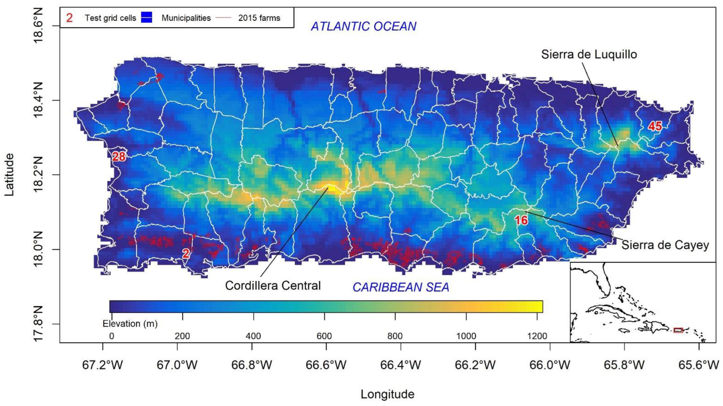
2.1. Study Area

The study area consists of the main island of the Commonwealth of Puerto Rico, which has a wide range of climate types. Precipitation ranges from 800 mm/year in the subtropical dry forest on the south coast to over 4300 mm/year [24] in the subtropical rainforest of El Yunque, which is part of the Sierra de Luquillo on the northeast of the island (Figure 1). The spatial variability of rainfall results from easterly to northeasterly winds interacting with the local orography. Large rainfall amounts fall north [24] of the mountain range, which runs predominantly east–west over central portions of the island known as the Cordillera Central and the Sierra de Cayey, which runs southeastward on the eastern side of the island. The rainfall maximum occurs over the Sierra de Luquillo mountains in the northeast where the El Yunque rainforest is located. A westerly sea-breeze front develops on the western side of the island, which converges with the predominant easterly winds, resulting in strong convection and high rainfall amounts in the northwest part of the island. A rain shadow occurs over most of the southern coast of the island. Rainfall has a bimodal distribution with the highest rainfall in May–early June and late July–November. A mid-summer drought (MSD) develops in late June through early July and, based on climate model simulations, has been found to be the combined result of increased aerosol concentrations from Saharan dust events and changes in vertical wind shear [25].
Low relative humidity, high temperatures, high wind speed, and high incoming solar radiation on the south coast result in high atmospheric evaporative demand compared to rainfall. The south-coast region is characterized by alluvial floodplains with highly fertile soils (mollisols), which are rich in organic matter and minerals [26]. This has made the region suitable for agriculture, which, owing to the relatively low annual rainfall, is dependent on irrigation. Of particular interest to water managers are potential future changes in water availability and water use across the island [4]. There is increasing concern about potential future conflicts among domestic and agricultural water uses on the southern coast of the island [4]. Therefore, it is important to quantify potential future agricultural water demand on irrigated farms and golf courses on the island, which are predominantly located in this southern region (Figure 1; [27]). Agriculture also occurs in the interior mountainous parts of the island, which receive high amounts of rainfall during the year so as not to require irrigation, but these areas may also be subjected to reductions in rainfall in the future [9].

2.2. Data

2.2.1. Gridded Historical Data

The Geostationary Operational Environmental Satellite-Puerto Rico Water and Energy Balance (GOES-PRWEB) dataset [28] provides daily gridded data for water and energy budget components at a 1 km resolution over Puerto Rico for the period 2009–2020. GOES-PRWEB provides estimates of daily rainfall, actual evapotranspiration, reference evapotranspiration (ETo) based on the FAO-56 (or ASCE) P-M equation (Equation (1) in Section 2.3), as well as data for five basic meteorological variables that are used in estimating ETo: daily maximum (Tmax) and minimum (Tmin) air temperature at 2 meter height, daily mean relative humidity (RHmean), daily mean incoming solar radiation at the land surface ( R s ), and 2 m-height wind speed ( u 2 ). Appendix S1 in Supplementary Materials summarizes the GOES-PRWEB computation of ETo from these five basic variables. GOES-PRWEB estimates actual ET based on the surface energy balance equation, as described by Harmsen et al. [28]. The GOES-PRWEB estimated ETo and its driving meteorological variables have been validated by Mecikalski and Harmsen [29] and Harmsen et al. [28,30] at a few stations on the island, supporting the use of GOES-PRWEB ETo in this study. For this study, GOES-PRWEB data for the period 2009–2017 is used.
The high-resolution regional statistical downscaled GPCC v7 for the Caribbean dataset (Herrera-Ault; [7,31]) provides estimates of monthly potential evapotranspiration based on the FAO-56 P-M equation [32] at an approximate resolution of 4 km. Although these data are referred to as potential evapotranspiration, Herrera and Ault [31] mention that this dataset refers to evapotranspiration from an idealized grass surface, that is, ETo. ETo data from this dataset show higher values than GOES-PRWEB from December to April and lower values than GOES-PRWEB the rest of the year. Besides Tmax and Tmin, Herrera-Ault does not provide data for the remaining variables required for ETo estimation using the FAO-56 P-M equation. This lack of availability of all the meteorological data needed for ETo estimation makes it impossible to investigate the causes of the differences in seasonality between the two datasets.

2.2.2. WRF Dynamically Downscaled Climate Change Projections

Bowden et al. [9] used the Weather Research and Forecasting (WRF) model to dynamically downscale historical (1985–2005) and future climate projections (2040–2060) for Puerto Rico and the U.S. Virgin Islands under the greenhouse gas emission scenario RCP8.5 for two GCMs from the Coupled Model Intercomparison Project phase 5 (CMIP5): (1) the Community Climate System Model (CCSM4 or CESM) and (2) the Centre National de Recherches Météorologiques-CERFACS (CNRM). Hourly output from the innermost model domain (domain 3 at 2-km resolution) was downloaded from the Bowden et al. [33], converted from Greenwich Meridian Time to local time (Atlantic Standard Time), and the five basic daily meteorological variables used for ETo estimation in GOES-PRWEB were computed and bilinearly interpolated to the 1-km GOES-PRWEB grid. Appendix S2 in Supplementary Materials has a description of the computation of daily meteorological data from hourly data.

2.3. Methods

Actual ET depends on various factors, including atmospheric evaporative demand, soil water availability, crop physiology, and management practices. Absent actual ET data, crop potential evapotranspiration (ETc) is often computed based on the potential evapotranspiration from a reference crop, typically grass or alfalfa, which is called reference evapotranspiration. Grass reference evapotranspiration is denoted as ETo and refers to a crop assumed to be 0.12 m in height, with an albedo of 0.23 and a daily surface resistance of 70 s/m [10]. Crop coefficients (Kc) are often used as multipliers to convert ETo to ETc (i.e., ETc = Kc ETo). ETo accounts primarily for weather conditions (i.e., atmospheric evaporative demand), and Kc accounts for the characteristics of a specific crop with respect to the reference grass under fully watered conditions [32]. Therefore, the crop coefficients incorporate many factors that distinguish a particular crop from the reference grass, including planting date, plant growth stage, leaf area, albedo or reflectivity, canopy resistance, soil and climate conditions, evaporation from soil, and crop management practices, among others [32]. In conditions of insufficient rainfall or irrigation and a deficit in soil moisture, the actual combined soil evaporation and plant transpiration (actual ET) will be lower than ETc. GOES-PRWEB estimates actual ET based on the surface energy balance equation, as described by Harmsen et al. [28]. In modeling applications, where actual ET cannot be estimated a priori but depends on the simulated hydrology, actual ET is often estimated from ETo using modified crop coefficients, which not only account for crop-type differences but also for water availability. Water stress coefficients, which are often defined as a function of soil water content and/or depth to the water table, can be applied as multiplicative correction factors to the standard crop coefficients for well-watered conditions [32] to estimate actual ET.
The ASCE standardized grass-reference Penman–Monteith evapotranspiration equation [10] for short grass on a daily timestep is given by:
E T o = 0.408   Δ   R n G + γ 900 T + 273 u 2 e s e a Δ + γ 1 + 0.34 u 2 ,
where ETo is the daily reference evapotranspiration (mm/day), R n is the net radiation at the crop surface (MJ/m2/day), G is the soil heat flux density at the soil surface (MJ/m2/day), which is generally small compared to R n beneath a fully vegetated reference surface, and hence, neglected for daily timesteps, T is the mean daily air temperature at 2 meters (°C), u 2 is the mean daily wind speed at 2 meters (m/s), e s is the saturation vapor pressure at 2 meters (kPa), e a is the mean actual vapor pressure at 2 meters (kPa), ∆ is the slope of the saturation vapor pressure–temperature curve (kPa/°C), and γ is the psychrometric constant (kPa/°C). Appendix S1 summarizes how each of these variables are estimated from five basic meteorological variables defined hereafter and available in GOES-PRWEB. When applied on a daily timestep, the ASCE standardized ETo equation is the same as the Food and Agriculture Organization paper number 56 (FAO-56) P-M equation [11].
A sensitivity analysis was performed for the ASCE ETo equation to determine the sensitivity of ETo to each of the five basic meteorological variables listed above. Neglecting higher-order terms, the sensitivity of ETo to changes (or errors) in each of the individual basic meteorological variables is quantified by means of non-dimensional relative sensitivity coefficients [34]:
S V i = E T o V i × V i E T o   ,
where V i is one of five basic meteorological variables (Tmax in °C, Tmin in °C, RHmean in %, R s in MJ/m2/day, or u 2 in m/s), i is the index for the variable (1–5), S V i is the relative SC for variable V i , and E T o V i is the partial derivative of ETo with respect to V i . A positive (negative) SC for a variable indicates that ETo will increase (decrease) as the variable increases and can be visualized as the slope of the tangent at the origin of the sensitivity curve. The derivatives, E T o V i , were derived analytically (Appendix S3 of the Supplementary Materials) and also derived numerically, and their linearity assessed by computing and plotting the percentage change in ETo due to +/− 5, 10, 15, 20, and 25% change in V i alone. This is done by changing the value of the variable of interest at each particular location on each day by a given percentage while keeping the remaining variables fixed at their observed value and computing the resulting change in ETo as a percentage. For RHmean, only negative percent changes were evaluated in order to keep it from exceeding 100%. It is expected that the analytically derived SCs will be closest to those derived based on +/− 5% perturbations for a particular variable. The range of variation in a meteorological variable over which the slope of the sensitivity curve is linear is also assessed. The larger the range of linearity, the smaller the error incurred when applying the point SCs over large changes in the meteorological variable.
The SCs are estimated based on daily GOES-PRWEB gridded meteorological data for the period 2009–2017 and averaged for each day or month of the year to obtain the average annual cycle of the SCs for each variable of interest at each grid cell. Timeseries of average SCs by day of the year will be presented at four representative locations on the island (Figure 1) that capture most of the distinct patterns of variation in the SCs as well as maps of long-term monthly average SCs.
When combined with a measure of the variability or measurement/estimation error in the basic meteorological variables, the SCs could be used to define monitoring priorities among the variables. The SCs could also be used to guide the prioritization of bias correction of meteorological output for ETo estimation from climate models. When combined with projections of the percent change in the basic meteorological variables, the SCs can aid in understanding past trends and future projected changes in ETo derived from observations and climate model output. Based on the chain rule, which helps differentiate composite functions, the combined contributions of fractional changes or errors in the basic meteorological variables to fractional changes or errors in ETo can be approximated by:
d E T o E T o = i S V i × d V i V i + e r r o r = i E T o V i × V i E T o   × d V i V i + e r r o r ,
where error is the approximation error.
An example application of the SCs and Equation (3) to understanding biases and potential future changes in ETo from 1985–2005 to 2040–2060 based on the dynamically downscaled climate projections for Puerto Rico by Bowden et al. [9] will be presented in this paper. Of particular interest are potential future changes to agricultural water demand on irrigated farms on the island, which are a function of future projected changes in precipitation and evaporative demand (ETo). As of the year 2015, most irrigated farms are located in the fertile semi-arid southern coast of Puerto Rico (Figure 1; [27]). The average annual cycle of the SCs and the contribution of projected changes in each of the basic meteorological variables to projected changes in ETo were calculated for all model grid cells whose center is located within a 2015 irrigated farm. No comprehensive gridded meteorological dataset including daily data for all the basic meteorological variables used in estimating ETo has been located for the simulated historical period 1985–2005; therefore, GOES-PRWEB data for 2009–2017 is used to examine potential biases in ETo calculated from downscaled model output and the contribution of individual meteorological variables to those biases.
Finally, the Pearson correlation coefficient (r) between long-term monthly average maps of SCs, the five basic meteorological variables, the aerodynamic and energetic components of ETo and their fractions (ETo,energetic, ETo,aerodynamic, ETo,energetic fraction, ETo,aerodynamic fraction, respectively, given by Equations (S1.1)–(S1.5) in the Supplementary Materials), rainfall, and elevation will be presented. The Pearson correlation coefficient is a measure of the strength of the linear association between two sets of data and will be used here to better understand how different variables affect or are correlated with ETo. Because the correlation coefficient is calculated between all the monthly maps, it captures both temporal and spatial correlations between the different fields. In the discussion, the correlation (or anti-correlation) between variables is considered moderate for absolute values of r of 0.50–0.69, high for absolute values of r of 0.70–0.89, and very high for absolute values of r of 0.90–1.00.

3. Results

Spatiotemporal variations in rainfall, ET, and other components of the hydrologic cycle in Puerto Rico will be presented as maps and seasonal and annual plots. Results of the sensitivity analysis will be presented as long-term (2009–2017) monthly average maps of SCs and timeseries of SCs at various locations. Results from the application of SCs to understand model biases and projected future changes in ETo based on dynamically downscaled climate model output will also be presented.

3.1. Spatiotemporal Variations in Rainfall and ET

On the basis of GOES-PRWEB data [28], it was found that annual rainfall (Figure 2a) and annual actual ET (Figure 2b) are similar in magnitude across large portions of the island. About 65% of rainfall on average island wide, and upwards of 90% in the south coast, returns to the atmosphere as evapotranspiration on an average year (Figure 2c). Only a small fraction of annual rainfall recharges the shallow aquifer (Figure 2e), while the fraction of annual rainfall that generates runoff is higher in areas with higher rainfall, such as on the central northwest part of the island and on the Sierra de Luquillo in the northeast (Figure 2f). Annual atmospheric evaporative demand, as quantified by ETo, is more than twice as high as annual rainfall over the south coast of Puerto Rico (Figure 2d), where agriculture has to rely on irrigation to meet the atmospheric evaporative demand. Low relative humidity, high temperatures, high wind speed, and high incoming solar radiation on the south coast result in high ETo compared to rainfall.
Figure 3a,b illustrate the annual cycle of monthly rainfall and ETo and Figure 3c illustrates the interannual variability of ETo at the 2015 irrigated farm locations. The bimodal distribution of rainfall is evident in Figure 3a, with the highest rainfall in May–early June and late July–November. The mid-summer drought (MSD) that develops in late June through early July is also evident. The annual cycle of monthly ETo. (Figure 3b) from GOES-PRWEB with peak values in July appears to match station-based estimates of ETo in Harmsen et al. [35] better than the Herrera-Ault ETo which peaks in March. This justifies our use of GOES-PRWEB ETo in this study.

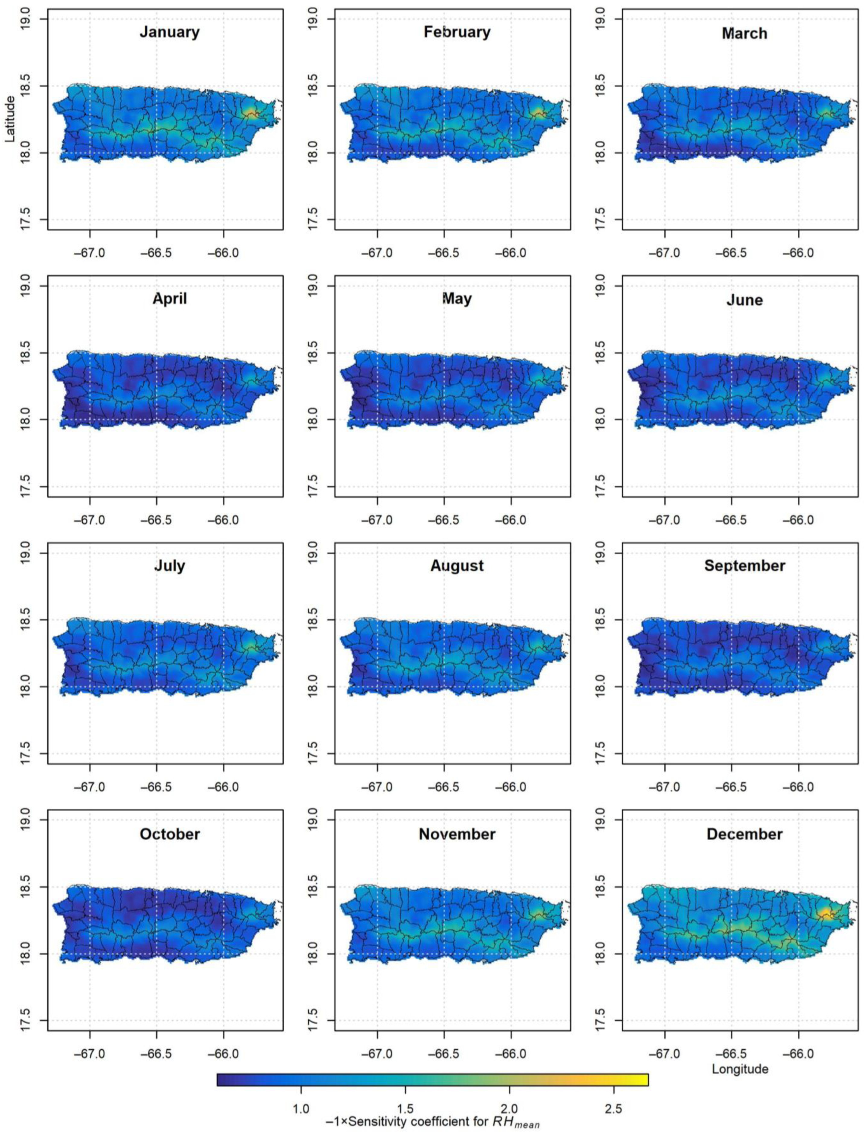
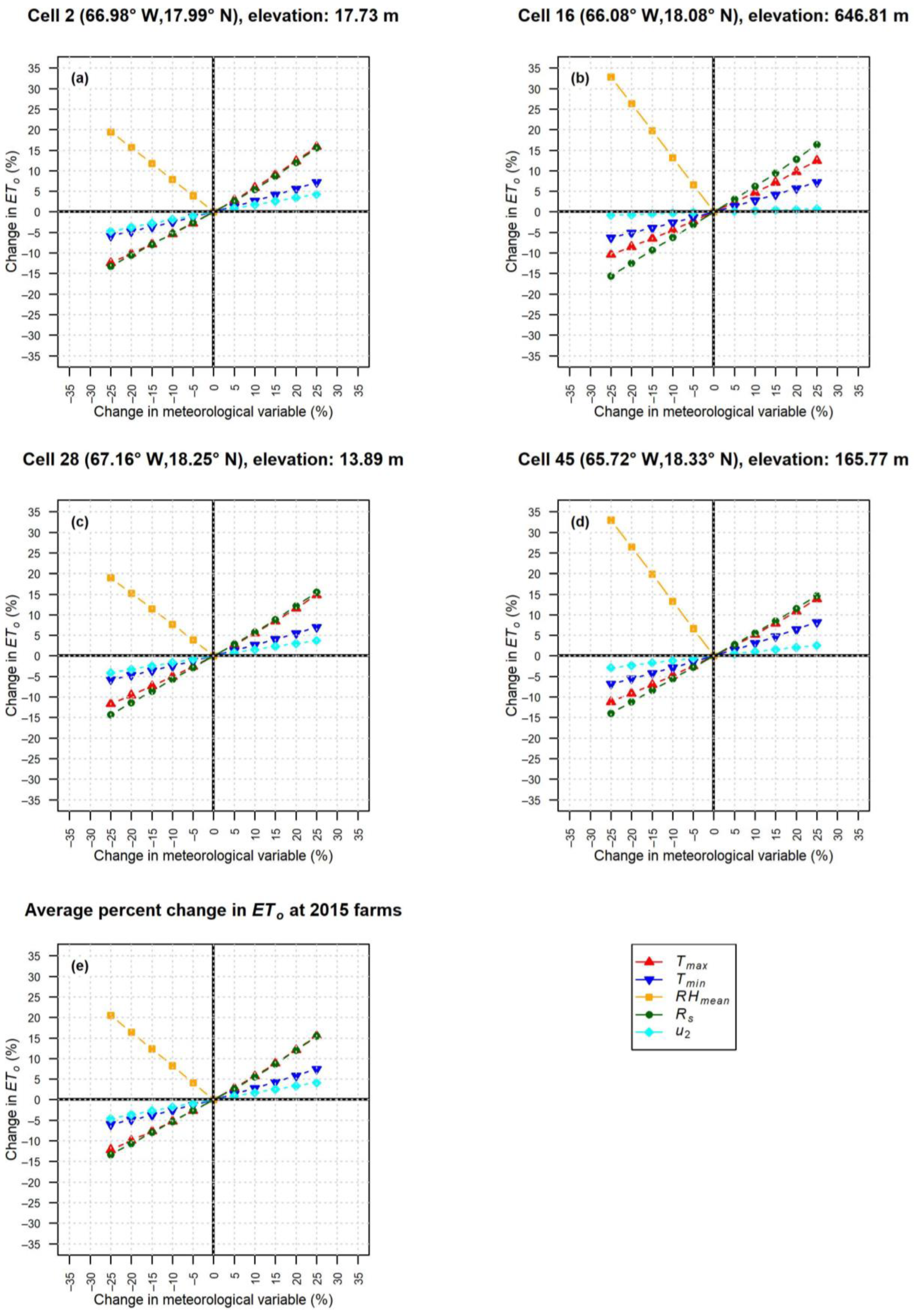
3.2. Sensitivity Coefficients

Sensitivity coefficients for ETo, with respect to each of the five basic meteorological variables, were computed analytically and numerically at each GOES-PRWEB grid cell for each day in the period 2009–2017. Maps of the long-term (2009–2017) monthly average sensitivity coefficients derived analytically are shown in Figure 4, Figure 5, Figure 6, Figure 7 and Figure 8. The maps derived numerically for a +/− 5% change in each meteorological variable (not shown) are very similar, corroborating the analytical calculations. The SC for RHmean is negative because an increase in atmospheric water content reduces ETo. To make the SC for RHmean of comparable magnitude to the SC of the other meteorological variables, it is multiplied by −1 in Figure 4. Island wide, ETo is most sensitive to RHmean, followed by Rs, Tmax, Tmin, and u 2 , with average absolute relative SCs of 0.98, 0.57, 0.50, 0.27, and 0.12, respectively. This overall ranking of sensitivities is similar to that found by Emeka et al. [18] based on relative sensitivities for the tropical rainforest climate of southern Nigeria, where precipitation ranges from 1200 to 3000 mm per year, similar to the range of annual precipitation in Puerto Rico (Figure 2a). The only exception is that in southern Nigeria, ETo was found to be most sensitive to Rs followed by RHmean in the non-monsoon season. The ranking of sensitivities also agrees well with that obtained by Gong et al. [12] for the Yangtze River Basin in China, especially during winter when the sensitivity to RHmean is higher than that of Rs and Tmean. Annual precipitation ranges from 400 in the upper Yangtze River Basin to 1600 mm in the lower basin [15]. Only the middle and lower portions of the Yangtze River Basin have annual precipitation comparable to that of some regions in Puerto Rico (Figure 2a).
Timeseries of SCs by day of the year averaged over the period 2009–2017 at the chosen four GOES-PRWEB grid cell locations (cells 2, 16, 28, 45; Figure 1) are shown in Figure 9. In addition, the average timeseries of SCs for the location of the farms as of 2015 shown in Figure 1 is also shown in Figure 9. The SC for RHmean (Figure 4 and Figure 9) dominates the sensitivity of ETo throughout most of the island, except for the western side of the island (cell 28 in Figure 1 and Figure 9), where the SC for Rs is as or more dominant during the summer. The SC for RHmean has a large amplitude annual cycle, especially along the Cordillera Central mountains and the Sierra de Luquillo with larger values and less day-to-day variability in the dry season than in the wet season. Coastal areas including the 2015 irrigated farm locations have a lower relative sensitivity to RHmean, with a less marked annual cycle than interior areas.
Higher SCs for Rs are apparent (Figure 5) along an interior band that goes from the northwest to the southeast on the island and generally coincides with more humid regions (Figure 2a), consistent with the findings of Tabari and Talaee [36] for Iran and Emeka et al. [18] for Nigeria. ETo is relatively less sensitive to Rs along the northeast coast and especially along the south coast. Although a clear seasonal cycle of higher relative sensitivity to Rs during the summer months is evident (Figure 5 and Figure 9), its amplitude is much smaller than that of RHmean. Although, overall, the SCs for Rs and Tmax are quite close on an island-wide basis (0.57 and 0.50, respectively), their spatial and temporal patterns are generally opposite (Figure 5, Figure 6 and Figure 9). ETo is relatively less sensitive to Tmax along interior mountainous regions of the island and during the summer months, and more sensitive along coastal areas, especially in the southern and western coasts during the dry season months. Seasonal variations in the relative sensitivity to Tmax are relatively minor, especially in mountainous areas (cell 45 in Figure 1 and Figure 9). Minimal spatial and temporal variation in the SCs for Tmin was found, with only slightly lower values in the western interior areas of the island from January to April and slightly higher values in coastal areas to the east (Figure 7).
Many similarities in the spatial and temporal patterns of SCs to u 2 (Figure 8) and the spatial and temporal patterns of SCs to Tmax (Figure 6) were found. However, ETo is much less sensitive to relative changes in u 2 than in Tmax (Figure 9). The relative sensitivity of ETo to changes in Tmax and u 2 is lower along humid and warm interior mountainous regions of the island and during the rainy summer months, and higher along coastal areas, especially in the southern coast during the dry season months. These findings are consistent with those of Emeka et al. [18] for Nigeria and Tabari and Talaee [36] for Iran. The lower sensitivity of ETo to changes in wind speed in humid and warm environments compared to its higher sensitivity in hot and dry environments is explained by Allen et al. [32]. In humid and warm conditions, such as in the interior mountains, the wind (no matter how intense) can only replace saturated air at the vegetation’s surface with air from above that is only slightly less saturated, thereby limiting potential increases in evapotranspiration. Increases in wind speed may, in fact, increase sensible heating more than evapotranspiration in these humid and warm environments, resulting in slightly negative SCs for u 2 at times (Figure 8 and cell 16 in Figure 9). In contrast, in hot and dry environments, such as the island’s south coast, increases in wind speed can increase the evapotranspiration rate more since the atmosphere is thirstier and has more energy available.
Figure 10 shows the percent change in ETo due to +/− 5, 10, 15, 20, and 25% changes in basic meteorological variables at selected GOES-PRWEB grid cell locations shown in Figure 1 and the average at the 2015 irrigated farm locations. The larger relative sensitivity of ETo to changes in RHmean compared to other variables is evident in the larger slope for the RHmean line. Linearity in the SCs is observed over the tested range of percentage changes in the basic meteorological variables at all grid cells, which means that the application of the SC values at the origin over a relatively wide range of changes in the meteorological variables is appropriate.
The Pearson correlation matrix is presented between long-term monthly maps of basic meteorological variables, their SCs, components of ETo, rainfall, and elevation (Table 1). The SC for RHmean has not been multiplied by −1 when calculating correlations. To aid in the discussion, Figures S1–S11 show maps of the long-term monthly average for the basic meteorological variables, rainfall, and components of ETo. The SC for RHmean (Figure 4 shows the SC for RHmean multiplied by −1) is highly anti-correlated to RHmean (Figure S1), specifically to the spatial pattern in RHmean. In other words, ETo is most sensitive to changes in RHmean in areas where RHmean already tends to be high and limiting, such as in the high-elevation areas of the Cordillera Central and the Sierra de Luquillo, where it exceeds about 82% on average (Figure S1). In these areas, lower Rs (Figure S2) also results in a lower contribution from ETo,energetic (Figure S7). The absolute value of the SC for RHmean is also highest in winter when aerodynamic effects become more important due to lower solar radiation. RHmean is highly anti-correlated to ETo,aerodynamic and ETo,aerodynamic fraction, as expected, since an increase in RHmean decreases the VPD and reduces these terms. RHmean is also highly correlated to elevation (Figure 1) and highly anti-correlated to Tmax reflecting the higher RHmean and the lower Tmax in the interior mountainous areas, and the opposite trends in coastal areas. RHmean is also highly anti-correlated to the SCs for Tmax and for u 2 . This is expected since these three variables act synergistically to increase ETo,aerodynamic, especially during winter.
The SC for Rs (Figure 5) is generally higher along the higher-elevation interior areas and moderately correlated to Rs (Figure S2). They are highly correlated in time (i.e., months with lowest Rs are also the months with lowest SC for Rs) but somewhat anti-correlated in space (i.e., areas with the lowest Rs in the interior mountains have the highest SC for Rs). The SC for Rs is moderately correlated to ETo,energetic (Figure S7), especially in time. The sensitivity to Rs is highest from northwest to southeast interior areas, especially in summer when Rs and ETo,energetic are at their highest and tend to dominate over aerodynamic effects (Figures S9 and S10). In winter, the aerodynamic term dominates more, so that Rs is not as important in driving ETo on the southwest coast for example (Figure 5). As expected, ETo,energetic (Figure S7) is very highly correlated to Rs and to elevation since Rs is moderately anti-correlated to elevation (Figure 1) due to the common presence of clouds at higher elevations. Rs is moderately correlated to Tmax and Tmin. This is most evident in the interior mountainous areas where Rs, Tmax, and Tmin tend to be the lowest. Rs is moderately correlated to the SC for RHmean (Figure 4) since Rs tends to be higher along coastal areas where the SC for RHmean is higher (less negative).
Rainfall from GOES-PRWEB was only found to be moderately correlated to the SC for Rs and ETo,energetic fraction. The correlation between rainfall and elevation was found to be quite low at only 0.02. Figure 2a shows two distinct areas of high rainfall—in the Sierra de Luquillo on the eastern side of the island, and in the northwest central part of the island (Figure 1). The spatial variability of rainfall results from easterly to northeasterly winds interacting with the local orography. However, rainfall appears to occur predominantly on the windward side of the mountains and not exactly at the locations with highest elevations. Even in the Sierra de Luquillo, the expectation of higher rainfall at higher elevations may not hold. Based on a relatively large set of rain gauges, Murphy et al. [37] found that the long-held assumption of precipitation increasing consistently with elevation within the Sierra de Luquillo does not hold. They found that leeward (western) watersheds in the mountains generally receive lower mean annual precipitation than windward (eastern) watersheds.
The SC for Tmax (Figure 6) is higher along the low-elevation coastal areas, especially along the south coast, and it is moderately correlated to Tmax (Figure S3). They are highly correlated spatially; however, they appear anti-correlated in time. That is, the cooler winter months with lower Tmax show a higher sensitivity to Tmax as the energetic term decreases and the aerodynamic term’s importance increases, especially along the southwest coast (Figures S9 and S10). Tmax (Figure S3), Tmin (Figure S4), and elevation (Figure 1) are very highly correlated due to lower temperatures in the interior mountain regions. Tmax stays relatively high in the southwest coast year-long, whereas Tmin is reduced during winter and early spring in the area, resulting in a higher daily temperature range in the area in winter and early spring. Tmax is moderately to highly correlated to both ETo,energetic (Figure S7) and ETo,aerodynamic (Figure S8) because it affects both terms; however, it appears to affect ETo and especially the aerodynamic component more in the winter when it acts synergistically with u 2 and RHmean to increase it, especially along coastal areas. Tmax is also highly correlated to the SCs for RHmean (Figure 4) and has a moderate correlation to the SC for u 2 (Figure 8). This is expected since these three variables act synergistically to increase ETo,aerodynamic, especially during winter. The SC for Tmin (Figure 7) is highly correlated to Tmin (Figure S4). The correlation is stronger in time than in space. Tmin is moderately correlated to both ETo,energetic (Figure S7) and ETo,aerodynamic (Figure S8) since it affects both terms.
The SC for u 2 (Figure 8) is generally higher along coastal areas and has no correlation to the spatial pattern in u 2 (Figure S5). As expected, u 2 is moderately correlated to ETo,aerodynamic (Figure S8); u 2 is also moderately correlated to the sensitivity coefficient for Tmin (Figure 7). The SCs for Rs (Figure 5) and for Tmax (Figure 6) are moderately anti-correlated. This is especially true in time (i.e., in winter months, the SC for Rs decreases while the SC for Tmax increases, especially in coastal areas), but also to a lesser extent in space (i.e., interior areas have the highest SCs for Rs and the lowest SC for Tmax). The SCs for Rs (Figure 5) and for u 2 (Figure 8) are highly anti-correlated. This is especially true in time (i.e., in winter months, the SC for Rs decreases while the SC for u 2 increases, especially in coastal areas), but also to a lesser extent in space (i.e., interior areas have the highest SCs for Rs and the lowest SC for u 2 ). The SCs for Tmax (Figure 6) and for u 2 are highly correlated in both space and time. The SC for RHmean (Figure 4) is moderately correlated to ETo,energetic (Figure S7) and has a moderate correlation to ETo,aerodynamic (Figure S8). The SC for Rs (Figure 5) is moderately correlated to ETo,energetic (Figure S7) and very highly correlated to ETo,energetic fraction (Figure S9), as expected.

3.3. Application

Timeseries of SCs are presented by day of the year (Figure 9e) at the GOES-PRWEB grid cells at the 2015 irrigated farms, most of which are located along the south coast (Figure 1). Compared to interior areas, the areas including the 2015 irrigated farm locations show a lower relative sensitivity to RHmean (Figure 4) with a less marked annual cycle. ETo is also relatively less sensitive to Rs (Figure 5) in these areas, especially during winter months when ETo becomes more sensitive to relative changes in Tmax (Figure 6). The relative sensitivity of ETo to changes in u 2 is lower than for other variables but higher along the southern coast than in other areas, especially during the dry season. In hot and dry environments, such as the south coast, increases in wind speed can increase the evapotranspiration rate more since the atmosphere has a lower moisture content and more energy available.
The lowest ETo,energetic fraction (Figure S9) and the highest ETo,aerodynamic fraction (Figure S10) occur in the south coast of Puerto Rico. This is due to this region having the highest Tmax (Figure S3) and the lowest RHmean (Figure S1) (which results in a high VPD) combined with moderate wind speeds in this area (Figure S5). These factors result in comparatively high ETo,aerodynamic (Figure S8) and ETo,aerodynamic fraction (Figure S10) compared to other areas. The low RHmean and relatively low cloudiness on the south coast also traps less longwave radiation in the atmosphere, reducing the net radiation, which would tend to reduce the energetic term. However, this effect appears to be counteracted by higher Rs (Figure S2) due to the lower cloudiness for a net result of higher incoming net radiation and higher ETo,energetic (Figure S7) compared to other areas.

3.3.1. Causes of Errors in Reference ET Estimated from Model Output for 1985–2005

Combining the average SCs at the 2015 irrigated farm locations on a monthly basis (Figure 11a) with the percent error in the simulated basic meteorological variables for the period 1985–2005 with respect to GOES-PRWEB for 2009–2017 according to Equation (3) gives the total contribution of each variable to errors in estimated ETo for the two downscaled GCMs (Figure 11b,c). The individual lines in these plots show the product of the SC for a particular basic meteorological variable times the percent error in the variable, which gives the contribution of that variable to the total error in ETo as a percentage. The brown line shows the total computed error in ETo ( d E T o E T o in Equation (3), as a percentage), and the black line shows the sum of the contributions from all the five basic meteorological variables to the total error in ETo ( i E T o V i × V i E T o   × d V i V i in Equation (3)). The difference between the black and brown lines is the approximation error (error in Equation (3)). The individual error components add up to large negative monthly biases in ETo of up to −21.1% for CNRM and −12.3% annually. The largest and most consistent contributors to those negative biases appear to be the well-documented [9] cold model biases for both Tmax and Tmin. However, biases in all five meteorological variables act synergistically to result in a large underestimation of ETo during October–December in CNRM. Despite ETo being most sensitive to relative errors in RHmean than in the other variables, smaller relative biases in RHmean in CNRM compared to other variables resulted in a smaller contribution of RHmean to errors in ETo.
In CESM, the cold biases for Tmax and Tmin are compensated by positive contributions to ETo bias from other meteorological variables during certain parts of the year, resulting in overall lower annual bias (−0.5%) than CNRM, and monthly biases ranging from −9.8% to 7.2%. Therefore, only bias correcting model output for precipitation and temperature, as is commonly done due to the widespread availability of observational gridded datasets for these two variables, is not always appropriate. Here, it would decrease the biases in ETo for CNRM but increase them for CESM. Although the existence of a cold bias in the downscaled models has been identified in other studies, it is important to note that some of the apparent errors in the other variables may be due to the different periods being compared between the model historical simulation and the observations.

3.3.2. Causes of Changes in Reference ET Estimated from Model Output for 2040–2060

The monthly SCs at the 2015 irrigated farm locations (Figure 11a) were also combined with the percent change in the simulated basic meteorological variables from 1985–2005 to 2040–2060 to obtain the total contribution of each variable to projected changes in ETo for the two downscaled GCMs (Figure 11d,e). The individual lines in these plots show the product of the SC for a meteorological variable times the percent change in the variable from 1985–2005 to 2040–2060, which gives the contribution of that variable to the total change in ETo as a percentage. The brown line shows the total computed change in ETo ( d E T o E T o in Equation (3), as a percentage), and the black line shows the sum of the contributions from all five basic meteorological variables to the total change in ETo ( i E T o V i × V i E T o   × d V i V i in Equation (3)). The difference between the black and brown lines is the approximation error (error in Equation (3)). Both models project an overall 5.6% increase in annual ETo mainly due to projected increases in Tmax and Tmin and a decrease in RHmean; however, the seasonality of the changes is different between the two models, as shown in Figure 11d,e. The projected decline in RHmean indicates a sub-Clausius–Clapeyron relationship (i.e., humidity increasing at rates lower than the 7% predicted by the Clausius–Clapeyron relationship; [38]) for the region which, together with the projected reductions in rainfall, may be a result of decreased moisture convergence into the region during the period 2040–2060. Despite ETo being most sensitive to relative changes in RHmean than in the other variables, smaller relative changes in RHmean in both models compared to Tmax and Tmin, result in similar contributions to changes in ETo from the three variables. The contribution of increases in u 2 to increases in ETo is also positive but minor. CNRM shows small changes in Rs during most months, while CESM shows a small decrease in Rs during most of the year. CESM projects larger increases in ETo during March, November, and December, increasing the potential for crop water stress during those times.

3.4. Limitations

Some key factors that were not considered in the application of the derived SCs to understanding potential future changes in ETo (and ETc) include increases in stomatal resistance and increases in photosynthesis in C3 plants and in C4 plants under drought [39] due to projected increases in atmospheric CO2 concentrations (CO2). These changes in plant physiology may counteract some of the expected increases in ETc from increased evaporative demand (ETo) due to higher temperatures [40]. Changes in stomatal resistance due to increases in CO2 can be informed by free-air carbon dioxide enrichment (FACE) experiments [39] and could be applied as modifications to the crop potential transpiration term to obtain estimates of ETc under future conditions, as in Kruijt et al. [41] and Scarpare et al. [42]. However, crop growth models are needed to better understand potential future changes in ET due to changes in plant biomass from increased photosynthesis and other factors, such as changes in stomatal resistance due to meteorological changes and changes in soil moisture, changes in planting dates and speed of plant growth, and feedbacks between these factors. For example, Scarpare et al. [42] used the CropSyst model to investigate potential future changes in ETc for five major irrigated crops in the Columbia Basin for 15 bias-corrected and statistically downscaled GCMs under the CMIP5 RCP8.5 scenario. Full irrigation was assumed to avoid crop water stress. For the 2090s, they found that changes in ETc ranged from −12.5% to +14.3% depending on the crop and the interplay of different meteorological, crop, and management factors. The application of a crop growth model to estimate changes in ETc for the main crops in Puerto Rico would help clarify potential future changes in agricultural irrigation requirements and aid water management planning efforts.
Additional sources of uncertainty include the effect of neglecting changes in soil heat flux density at the soil surface and changes in water heat flux density over areas with ponding water, which may be important during advective conditions such as cold fronts. In addition, there is an assumption that GOES-PRWEB meteorological and ETo data are reasonably accurate compared to observations, which may not necessarily be the case given that some of the data are derived from climate models, as described in Harmsen et al. [28]. As previously mentioned, the GOES-PRWEB estimated ETo, and its driving meteorological variables have been validated by Mecikalski and Harmsen [29] and Harmsen et al. [28,30] at a few stations on the island. The GOES-PRWEB precipitation and Tmax and Tmin fields have also been validated at stations throughout the island. However, efforts to validate the GOES-PRWEB dataset in a more comprehensive manner have been limited in particular by the lack of homogeneous, high-quality humidity, solar radiation, and wind speed data at a large number of stations on the island. For solar radiation in particular, some of the existing station data can show sensor issues, such as change points and drifts. In addition, at stations along the interior of the island, the upper envelope of daily solar radiation values is often well below a reasonable clear-sky radiation curve for the time of year, indicating that the station may be shaded by the local canopy or nearby obstructions (buildings, topographic features) for the majority of the year.
Similar concerns occur for wind speed data and are exacerbated by the lack of documented (changes in) sensor heights at meteorological stations. The sensitivity of ETo to changes in RHmean has been found to increase with increasing wind speed [12]. This is consistent with our finding of moderate autocorrelation between SC for RHmean and u 2 (r of −0.39 in Table 1) which means that as u 2 increases, the SC for RHmean becomes more negative (i.e., the absolute of the SC for RHmean increases). Therefore, errors in u 2 from GOES-PRWEB may affect the relative ranking of SCs across meteorological variables. In particular, an overestimation of u 2 in GOES-PRWEB would result in an overestimation of the SC for RHmean, which was found to be the meteorological variable with the highest relative sensitivity. For this reason, in Appendix S5, wind-speed records at stations throughout the island were compared with GOES-PRWEB wind speeds at the grid cell closest to each station (Table S1 and Figure S12). When sensor height information is available at a station (Table S1), it was used to convert the wind speeds to 2 m heights using the relationship in [10] for consistency with u 2 from GOES-PRWEB. Generally, wind sensors are installed at meteorological stations at 2 to 10 m heights, for which conversion factors to 2 m (based on [10]) range from 1 to 0.75, respectively. Therefore, when sensor height information is not available, a discrepancy of up to about 25% between station wind speeds and u 2 from GOES-PRWEB can be expected on average.
Figure S12b shows that the percent difference between GOES-PRWEB u 2 and sensor wind speed (converted to 2 m when possible) ranges between −23% and 225%. Notably, 16 out of 22 stations have percent differences between +/− 35%, which appear reasonable. However, high percent differences are observed at some stations along the southwest and southeast coasts and along the interior of the island. Furthermore, some of these stations with the higher percent differences are relatively close to other stations with lower percent differences, such as at the Yabucoa stations for example. These large discrepancies in percent differences within short distances may be due to various reasons, including incorrect measurement units, coordinates, or sensor height reported for the station, station sheltering, comparison of 1 km wind speeds from GOES-PRWEB versus point values, and large gradients occurring within small areas. The Global Wind Atlas [43] is a web-based application that provides estimates of wind speed for wind power generation worldwide. It uses the WRF model to downscale reanalysis data in the ERA5 dataset from the European Centre for Medium-Range Forecasts (ECMWF; [44]). The resulting 3 km wind speeds are then generalized and applied to a microscale modeling system to determine local wind climates at 250 m resolution at heights ranging from 10 to 200 m. The microscale model considers orography, roughness and roughness-change effects, including speed-up effects as the wind moves up a mountain or hill. The Global Wind Atlas shows a large gradient in the annual average 10 m wind speed from coastal to offshore areas of Puerto Rico and high variability in wind speeds over mountainous areas resulting from changes in roughness and orography. The 1 km GOES-PRWEB dataset is not expected to capture these localized changes. This likely explains the large changes in wind speed performance over small distances and the overestimation of wind speeds in GOES-PRWEB at interior stations.
Due to the uncertainty in wind speeds and the potential for its overestimation in GOES-PRWEB at some station locations, a sensitivity analysis was performed on the SCs where GOES-PRWEB u 2 was multiplied by factors equal to 0.67 and 0.5 to counteract possible overestimation of wind speeds in GOES-PRWEB by 50% and 100%, respectively. This sensitivity analysis represents the worst-case scenario, where it is assumed that the GOES-PRWEB u 2 is overestimated island wide, when Figure S12 shows that is clearly not the case. Results from this sensitivity analysis are shown in Appendix S5, where Figure 9 is recreated for the two factors (Figures S13 and S14; Table S2). As the wind speed is reduced, the SC for RHmean decreases and the SC for Rs increases. At some locations, such as cells 16 and 45 (Figure 1), the SC for RHmean remains mostly larger than the SC for Rs throughout the year when 0.67 u 2 is used (Figure S13), but only in the winter months when 0.5 u 2 is used (Figure S14). In the case when 0.67 u 2 is used, the SC for RHmean becomes comparable to the SC for Rs at many locations throughout the island, whereas when 0.5 u 2 is used, it becomes smaller than the SC for Rs, as reflected in the island-wide average SCs (Table S2).
As observed in Figure 3c, it was also found that the standard deviation of annual ETo at the location of 2015 irrigated farms and golf courses is much higher for GOES-PRWEB (97.0 mm/year for 2009–2017) than for the two downscaled climate models (35.7 and 35.6 mm/year for CESM, and CNRM, respectively, in the period 1985–2005) and the Herrera-Ault dataset (24.6 mm/year for 1985–2005). The larger interannual variability in GOES-PRWEB ETo may be due to the switch of datasets used in its derivation, as described by Harmsen et al. [28]. As previously discussed, the annual cycle of station-based estimates of ETo appears to match that of GOES-PRWEB better than that of Herrera-Ault (Figure 3b), with peak values in July as in GOES-PRWEB rather than in March as in Herrera-Ault. Since the exact magnitude of interannual variability of ETo in the study area is unknown, and the downscaled climate models show interannual variability within the range of the two observational datasets, it may be sensible to bias correct model-based ETo using GOES-PRWEB on monthly timescales only (i.e., no corrections for interannual variability).

4. Discussion

It was found that the SC for RHmean dominates the sensitivity of ETo throughout most of the island, even more so than the SCs for Rs and Tmax. This is because the high relative humidity over most of the island currently limits ETo and there is plenty of energy (Rs and Tmax) available for ETo in most areas during most of the year. The SC for RHmean has a large-amplitude annual cycle, especially along the Cordillera Central mountains and the Sierra de Luquillo with larger values and less day-to-day variability in the dry season than in the wet season. Coastal areas, including the 2015 irrigated farm locations, show a lower relative sensitivity to RHmean, with a less marked annual cycle than interior areas. The overall ranking of sensitivities found in our study (SC for RHmean > SC for Rs > SC for Tmax > SC for Tmin > SC for u 2 ) is similar to that obtained for the tropical rainforest climate of southern Nigeria [18] and for the Yangtze River Basin in China [12]. However, the SCs are not very meaningful on their own unless combined with a measure of the variability measurement/estimation error or changes in the basic meteorological variables with time.
Our main objective in deriving SCs for Puerto Rico was to guide the prioritization of bias correction of meteorological output for ETo estimation from dynamically downscaled climate projections, which can then be used to drive a soil-moisture water-balance model [2] for estimating future agricultural irrigation requirements on the island. This objective was met by applying the SCs to understand the sources of error and potential future changes in ETo estimated from downscaled model output at the 2015 irrigated farm locations. The results illustrate how the ranking of variable importance may change when the SCs are combined with estimates of error or change in meteorological variables. For example, despite ETo being most sensitive to relative errors in RHmean, relative biases in RHmean in the CNRM model are small compared to other variables. This results in a smaller contribution of RHmean to errors in CNRM-estimated ETo. Similarly, despite ETo being most sensitive to relative changes in RHmean than in the other variables, smaller relative future changes in RHmean compared to Tmax and Tmin in both climate models result in similar contributions to future changes in ETo from the three variables.
For the period 2040–2060, it was found that both climate models project an overall 5.6% increase in annual ETo over the 2015 irrigated farm locations with respect to the historical period 1985–2005. This increase in ETo is primarily a result of projected increases in Tmax and Tmin and a decrease in RHmean, with differences in the seasonality of changes between the two models. Absent compensatory increases in rainfall and/or a compensatory decrease in ETo due to stomatal closure as CO2 increases, the future increase in ETc resulting from the 5.6% increase in ETo may have to be met by an additional volume of irrigation. Future research could attempt to estimate the additional agricultural irrigation requirements and their sensitivity to various bias-correction choices.
Various limitations of the current study are highlighted in the results. They include uncertainties in the stomatal and plant-growth responses to projected increases in atmospheric CO2, uncertainties in crop suitability under climate change, the effect of neglecting changes in soil and water heat fluxes in the ETo equation, and the lack of sufficient meteorological data at weather stations to corroborate meteorological data and ETo estimates and the derived sensitivity coefficients. The development of reliable homogeneous spatially distributed long-term observational datasets of meteorological and hydrological variables is imperative for improving the understanding of drivers of hydrological processes, evaluating model performance, and for bias correction of model output.

Supplementary Materials

The following supporting information can be downloaded at: https://www.mdpi.com/article/10.3390/hydrology10050101/s1, Appendix S1: Aerodynamic and energetic components of the ASCE standardized reference evapotranspiration (ETo) equation; Appendix S2: Computation of daily meteorological variables from hourly WRF output; Appendix S3: Analytical sensitivity coefficient equations; Appendix S4: Maps of long-term (2009–2017) monthly average meteorological variables and ETo components; Appendix S5: Performance of GOES-PRWEB wind speed at 2 meters and sensitivity to errors in wind speed; Figure S1: Long-term (2009–2017) monthly average mean relative humidity (RHmean); Figure S2: Long-term (2009–2017) monthly average incoming solar radiation (Rs); Figure S3: Long-term (2009–2017) monthly average maximum air temperature (Tmax); Figure S4: Long-term (2009–2017) monthly average minimum air temperature (Tmin); Figure S5: Long-term (2009–2017) monthly average wind speed ( u 2 ); Figure S6: Long-term (2009–2017) monthly average daily rainfall rate; Figure S7: Long-term (2009–2017) monthly average energetic component or reference evapotranspiration (ETo,energetic); Figure S8: Long-term (2009–2017) monthly average aerodynamic component of reference evapotranspiration (ETo,aerodynamic); Figure S9: Long-term (2009–2017) monthly average energetic fraction of reference evapotranspiration (ETo,energetic fraction); Figure S10: Long-term (2009–2017) monthly average aerodynamic fraction of reference evapotranspiration (ETo,aerodynamic fraction); Figure S11: Long-term (2009–2017) monthly average daily evapotranspiration (ETo); Figure S12: (a) Location of stations with homogeneous wind speed data in Puerto Rico; (b) Percent difference, and (c) coefficient of determination (R2), between GOES-PRWEB and station wind speeds converted to 2-m height according to [10] when sensor elevation data are available; Figure S13: Daily timeseries of sensitivity coefficients (SCs) with wind speed multiplied by 0.67; Figure S14: Daily timeseries of sensitivity coefficients (SCs) with wind speed multiplied by 0.5; Table S1: Stations with homogeneous wind speed data in Puerto Rico; Table S2: Island-wide average absolute relative SCs for case with original GOES-PRWEB 2 m wind speeds and wind speeds multiplied by factors equal to 0.5 and 0.67. References [45,46,47,48,49,50] are cited in the supplementary materials.

Author Contributions

Conceptualization, M.I.-O.; methodology, M.I.-O.; software, M.I.-O.; validation, M.I.-O.; formal analysis, M.I.-O.; investigation, M.I.-O.; resources, M.I.-O.; data curation, M.I.-O. and E.W.H.; writing—original draft preparation, M.I.-O.; writing—review and editing, M.I.-O. and E.W.H.; visualization, M.I.-O.; supervision, M.I.-O. and E.W.H.; project administration, M.I.-O.; funding acquisition, M.I.-O. All authors have read and agreed to the published version of the manuscript.

Funding

This research was partially funded by the USGS, USDA-NIFA (W4128), and NSF (grant 1832576). Findings, opinions, or conclusions expressed in this paper do not necessarily reflect those of the USDA or NSF.

Data Availability Statement

GOES-PRWEB data can be found here: https://pragwater.com (accessed on 31 August 2021). Weather Research and Forecasting (WRF): Puerto Rico and US Virgin Islands Dynamical Downscaled Climate Change Projections are publicly available at https://doi.org/10.5066/F7GB23BW (accessed on 23 March 2021).

Conflicts of Interest

The authors declare no conflict of interest. The funders had no role in the design of the study; in the collection, analyses, or interpretation of data; in the writing of the manuscript; or in the decision to publish the results.

References

  1. Puerto Rico Institute of Statistics. Food Security in Puerto Rico, Calendar Year 2015. 2019. Available online: https://estadisticas.pr/files/Comunicados/Seguridad%20Alimentaria%20en%20Puerto%20Rico%20-%20Final%20%28300519%29.pdf (accessed on 20 July 2022).
  2. Molina-Rivera, W.L.; Irizarry-Ortiz, M.M. Estimated water withdrawals and use in Puerto Rico. U.S. Geol. Surv. Open-File Rep. 2021, 2021-1060, 1–38. [Google Scholar]
  3. Puerto Rico Planning Board. Memorial of the land use plan, Guide for the Classification of Territories. 2015. Available online: https://www.sciencebase.gov/catalog/item/576bfe89e4b07657d1a26ee5 (accessed on 8 February 2023).
  4. Puerto Rico Department of Natural and Environmental Resources. Integrated water resources plan for Puerto Rico. 2016. Available online: https://drna.pr.gov/wp-content/uploads/formidable/PIRA-2016.pdf (accessed on 8 February 2023).
  5. Harmsen, E.W.; Howard-Harmsen, R. Agricultural Water Management and Puerto Rico’s Food Insecurity. Ethos Gubernamental. Special Edition. September 2019. Available online: https://academic.uprm.edu/hdc/HarmsenPapers/Harmsen_and_Harmsen_Ethos.pdf (accessed on 18 July 2022).
  6. NOAA (National Oceanographic and Atmospheric Administration). National Integrated Drought Information System. Available online: https://www.drought.gov/states/puerto-rico (accessed on 20 July 2022).
  7. Herrera, D.A.; Ault, T.R.; Fasullo, J.T.; Coats, S.J.; Carrillo, C.M.; Cook, B.I.; Park Williams, A. Exacerbation of the 2013–2016 pan-Caribbean drought by anthropogenic warming. J. Geophys. Res. 2018, 45, 10619–10626. [Google Scholar] [CrossRef] [PubMed]
  8. Khalyani, A.H.; Gould, W.A.; Harmsen, E.; Terando, A.; Quinones, M.; Collazo, J.A. Climate change implications for tropical islands: Interpolating and interpreting statistically downscaled GCM projections for management and planning. J. Appl. Meteorol. Climatol. 2016, 55, 265–282. [Google Scholar] [CrossRef]
  9. Bowden, J.; Terando, A.J.; Misra, V.; Wootten, A.; Bhardwaj, A.; Boyles, R.; Gould, W.; Collazo, J.A.; Spero, T.L. High-resolution dynamically downscaled rainfall and temperature projections for ecological life zones within Puerto Rico and for the U.S. Virgin Islands. Int. J. Climatol. 2021, 41, 1305–1327. [Google Scholar] [CrossRef]
  10. ASCE (American Society of Civil Engineers); EWRI (Environmental and Water Resources Institute). Task Committee on Standardization of Reference Evapotranspiration. The ASCE standardized reference evapotranspiration equation. 2005. Available online: https://ascelibrary.org/doi/book/10.1061/9780784408056 (accessed on 20 April 2023).
  11. Irmak, S.; Payero, J.O.; Martin, D.L.; Irmak, A.; Howell, T.A. Sensitivity analyses and sensitivity coefficients of standardized daily ASCE Penman–Monteith equation. J. Irrig. Drain Eng. 2006, 132, 564–578. [Google Scholar] [CrossRef]
  12. Gong, L.; Xu, C.-y.; Chen, D.; Halldin, S.; Chen, Y.D. Sensitivity of the Penman–Monteith reference evapotranspiration to key climatic variables in the Changjiang (Yangtze River) basin. J. Hydrol. 2006, 329, 620–629. [Google Scholar] [CrossRef]
  13. McKenney, M.S.; Rosenberg, N.J. Sensitivity of some potential evapotranspiration estimation methods to climate change. Agric. For. Meteorol. 1993, 64, 81–110. [Google Scholar] [CrossRef]
  14. Debnath, S.; Adamala, S.; Raghuwanshi, N.S. Sensitivity analysis of FAO-56 Penman–Monteith method for different agro-ecological regions of India. Environ. Process. 2015, 2, 689–704. [Google Scholar] [CrossRef]
  15. Cao, L.; Zhang, Y.; Shi, Y. Climate change effect on hydrological processes over the Yangtze River basin. Quat. Int. 2011, 244, 202–210. [Google Scholar] [CrossRef]
  16. Liu, Q.; Yang, Z.; Cui, B.; Sun, T. The temporal trends of reference evapotranspiration and its sensitivity to key meteorological variables in the Yellow River Basin, China. Hydrol. Process. 2010, 24, 2171–2181. [Google Scholar] [CrossRef]
  17. Biazar, S.M.; Dinpashoh, Y.; Singh, V.P. Sensitivity analysis of the reference crop evapotranspiration in a humid region. Environ. Sci. Pollut. Res. 2019, 26, 32517–32544. [Google Scholar] [CrossRef] [PubMed]
  18. Emeka, N.; Ikenna, O.; Okechukwu, M.; Chinenye, A.; Emmanuel, E. Sensitivity of FAO Penman–Monteith reference evapotranspiration (ETo) to climatic variables under different climate types in Nigeria. J. Water Clim. Change 2021, 12, 858–878. [Google Scholar] [CrossRef]
  19. Hou, L.-g.; Zou, S.-b.; Xiao, H.-l.; Yang, Y.-g. Sensitivity of the reference evapotranspiration to key climatic variables during the growing season in the Ejina oasis northwest China. SpringerPlus 2013, 2 (Suppl. S1), S4. [Google Scholar] [CrossRef]
  20. Luo, Y.; Gao, P.; Mu, X. Influence of meteorological factors on potential evapotranspiration in Yanhe River Basin, China. Water 2021, 13, 1222. [Google Scholar] [CrossRef]
  21. Wang, T.; Zhang, J.; Sun, F.; Liu, W. Pan evaporation paradox and evaporative demand from the past to the future over China: A review. WIREs Water 2017, 4, e1207. [Google Scholar] [CrossRef]
  22. Peterson, T.; Golubev, V.S.; Groisman, P.Y. Evaporation losing its strength. Nature 1995, 377, 687–688. [Google Scholar] [CrossRef]
  23. Roderick, M.L.; Rotstayn, L.D.; Farquhar, G.D.; Hobbins, M.T. On the attribution of changing pan evaporation. Geophys. Res. Lett. 2007, 34, 251–270. [Google Scholar] [CrossRef]
  24. USGS (U.S. Geological Survey). Climate of Puerto Rico. 2016. Available online: https://www.usgs.gov/centers/caribbean-florida-water-science-center-%28cfwsc%29/science/climate-puerto-rico (accessed on 20 July 2022).
  25. Angeles, M.E.; González, J.E.; Ramírez-Beltrán, N.D.; Tepley, C.A.; Comarazamy, D.E. Origins of the Caribbean rainfall bimodal behavior. J. Geophys. Res. 2010, 115, D11106. [Google Scholar] [CrossRef]
  26. Muñoz, M.M.; Lugo, W.I.; Santiago, C.; Matos, M.; Ríos, S.; Lugo, J. Taxonomic Classification of the Soils of Puerto Rico, 2017. University of Puerto Rico, Mayagüez Campus, College of Agricultural Sciences, Agricultural Experiment Station Bulletin 313. January 2018. Available online: https://www.uprm.edu/tamuk/wp-content/uploads/sites/299/2019/06/Taxonomic_classification_soils_PR_2018_reduced.pdf (accessed on 20 July 2022).
  27. Dixon, J.F.; Molina-Rivera, W.L.; Irizarry-Ortiz, M.M.; Christesson, K.R. Spatial and Tabular Datasets of Water Withdrawals and Use in Puerto Rico, 2015. U.S. Geological Survey data release 2021. Available online: https://www.sciencebase.gov/catalog/item/600aec34d34e162231fb26d9 (accessed on 9 August 2022).
  28. Harmsen, E.W.; Mecikalski, J.R.; Reventos, V.J.; Alvarez Perez, E.; Uwakweh, S.S.; Adorno Garcia, C. Water and energy balance model GOES-PRWEB: Development and Validation. Hydrology 2021, 8, 113. [Google Scholar] [CrossRef]
  29. Mecikalski, J.R.; Harmsen, E.W. The use of visible geostationary operational meteorological satellite imagery in mapping the water balance over Puerto Rico for water resource management. In Satellite Information Classification and Interpretation; Rustamov, R.B., Ed.; IntechOpen: London, UK, 2019. [Google Scholar]
  30. Harmsen, E.W.; Tosado Cruz, P.; Mecikalski, J.R. Calibration of selected pyranometers and satellite derived solar radiation in Puerto Rico. Int. J. Renew. Energy Technol. 2014, 5, 43–54. [Google Scholar] [CrossRef]
  31. Herrera, D.; Ault, T. Insights from a new high-resolution drought Atlas for the Caribbean spanning 1950–2016. J. Clim. 2017, 30, 7801–7825. [Google Scholar] [CrossRef]
  32. Allen, R.G.; Pereira, L.S.; Raes, D.; Smith, M. Crop evapotranspiration: Guidelines for computing crop water requirements. FAO Irrig. Drain. Paper 1998, 56. Available online: https://www.fao.org/3/x0490e/x0490e00.htm (accessed on 18 July 2022).
  33. Bowden, J.; Wootten, A.; Terando, A.; Boyles, R. Weather Research and Forecasting (WRF): Puerto Rico and US Virgin Islands Dynamical Downscaled Climate Change Projections. U.S. Geological Survey Data Release 2018. Available online: https://www.sciencebase.gov/catalog/item/5977b95de4b0ec1a4888e493 (accessed on 23 March 2021).
  34. McCuen, R.H. A sensitivity and error analysis of procedures for estimating evaporation. Water Resour. Bull. 1974, 10, 486–498. [Google Scholar] [CrossRef]
  35. Harmsen, E.W.; Goyal, M.R.; Torres-Justiniano, S. Estimating evapotranspiration in Puerto Rico. J. Agric. Univ. Puerto Rico 2002, 86, 35–54. [Google Scholar] [CrossRef]
  36. Tabari, H.; Talaee, P.H. Sensitivity of evapotranspiration to climatic change in different climates. Glob. Planet. Change 2014, 115, 16–23. [Google Scholar] [CrossRef]
  37. Murphy, S.; Stallard, R.F.; Scholl, M.A.; González, G.; Torres-Sánchez, A.J. Reassessing rainfall in the Luquillo Mountains, Puerto Rico: Local and global ecohydrological implications. PLoS ONE 2017, 12, e0180987. [Google Scholar] [CrossRef] [PubMed]
  38. Koutsoyiannis, D. Revisiting the global hydrological cycle: Is it intensifying? Hydrol. Earth Syst. Sci. 2020, 24, 3899–3932. [Google Scholar] [CrossRef]
  39. Ainsworth, E.A.; Long, S.P. 30 years of free-air carbon dioxide enrichment (FACE): What have we learned about future crop productivity and its potential for adaptation? Glob. Change Biol. 2020, 27, 27–49. [Google Scholar] [CrossRef]
  40. Islam, A.; Ahuja, L.R.; Garcia, L.A.; Ma, L.; Sassendran, A.S. Modeling the effect of elevated CO2 and climate change on reference evapotranspiration in the semi-arid Central Great Plains. Trans. ASABE 2012, 55, 2135–2146. [Google Scholar] [CrossRef]
  41. Kruijt, B.; Witte, J.-P.M.; Jacobs, C.; Kroon, T. Effects of rising atmospheric CO2 on evapotranspiration and soil moisture: A practical approach for the Netherlands. J. Hydrol. 2008, 349, 257–267. [Google Scholar] [CrossRef]
  42. Scarpare, F.V.; Rajagopalan, K.; Liu, M.; Nelson, R.L.; Stöckel, C.O. Evapotranspiration of irrigated crops under warming and elevated atmospheric CO2: What is the direction of change? Atmosphere 2022, 13, 163. [Google Scholar] [CrossRef]
  43. Global Wind Atlas Version 3.0. Available online: https://globalwindatlas.info/en/area/Puerto%20Rico/ (accessed on 30 January 2023).
  44. Hersbach, H.; Bell, B.; Berrisford, P.; Hirahara, S.; Horányi, A.; Muñoz-Sabater, J.; Nicolas, J.; Peubey, C.; Radu, R.; Schepers, D.; et al. The ERA5 global reanalysis. Q. J. R. Meteorolog. Soc. 2020, 146, 1999–2049. [Google Scholar] [CrossRef]
  45. Wallace, J.M.; Hobbs, P.V. Atmospheric Science—An Introductory Survey, 2nd ed.; Elsevier: New York, NY, USA, 2006; p. 483. [Google Scholar]
  46. American Meteorological Society. Glossary of Meteorology. 2012. Available online: https://glossary.ametsoc.org/wiki/Mixing_ratio (accessed on 8 February 2023).
  47. CariCOOS (Caribbean Coastal Ocean Observing System). Weather Flow Mesonet Meteorological Station Aggregation Data. Available online: http://52.55.122.42/thredds/caricoos_mesonet_agg.html (accessed on 13 September 2021).
  48. IOOS (Integrated Ocean Observing System). Environmental Sensor Map. Available online: https://sensors.ioos.us/#map (accessed on 18 November 2021).
  49. NOAA (National Oceanic and Atmospheric Administration); NCEI (National Centers for Environmental Information). Global Summary of the Day—GSOD. User Engagement and Services Branch. DOC/NOAA/NESDIS/NCDC > National Climatic Data Center, NESDIS, NOAA, U.S. Department of Commerce. Available online: https://www.ncei.noaa.gov/cdo-web/ (accessed on 16 November 2021).
  50. WRCC (Western Regional Climate Center). National Interagency Fire Center Remote Automatic Weather Stations (RAWS). Available online: https://raws.dri.edu/prF.html (accessed on 10 November 2021).
Figure 1. Study area consisting of the main island of Puerto Rico. Elevation in meters is shown. The white lines show the boundaries of the municipalities in Puerto Rico, and the red lines show the boundaries of irrigated farms in 2015. Numbers indicate the location of Geostationary Operational Environmental Satellite-Puerto Rico Water and Energy Balance (GOES-PRWEB) 1 km-scale grid cells at which timeseries of sensitivity coefficients will be presented in detail. Base for main map from 1:20,000 USGS Digital Line Graphs municipality boundaries. Base for inset map is from version 1.4.0 of Natural Earth data, country boundaries 1:10 m. Both are in geographic coordinate system and World Geodetic System 1984 datum.
Hydrology 10 00101 g001
Figure 2. (a) Annual rainfall (mm/year); (b) annual actual ET (mm/year); (c) ratio of annual actual ET to rainfall; (d) ratio of annual Penman–Monteith ETo to rainfall; (e) ratio of annual aquifer recharge to rainfall; and (f) ratio of annual runoff to rainfall for Puerto Rico based on Geostationary Operational Environmental Satellite-Puerto Rico Water and Energy Balance (GOES-PRWEB) data for 2009–2017. The black lines show the location of the municipalities in Puerto Rico.
Hydrology 10 00101 g002
Figure 3. (a) Annual cycle of rainfall (mm/mo.); (b) annual cycle of ETo (mm/mo.); (c) annual ETo (mm/year) from Geostationary Operational Environmental Satellite-Puerto Rico Water and Energy Balance (GOES-PRWEB), Herrera-Ault dataset, and WRF dynamically downscaled climate models at the 2015 irrigated farm locations.
Hydrology 10 00101 g003
Figure 4. Long-term (2009–2017) monthly average sensitivity coefficients, multiplied by −1, for mean relative humidity (RHmean). The black lines show the location of the municipalities in Puerto Rico.
Hydrology 10 00101 g004
Figure 5. Long-term (2009–2017) monthly average sensitivity coefficients for solar radiation (Rs). The black lines show the location of the municipalities in Puerto Rico.
Hydrology 10 00101 g005
Figure 6. Long-term (2009–2017) monthly average sensitivity coefficients for daily maximum air temperature (Tmax). The black lines show the location of the municipalities in Puerto Rico.
Hydrology 10 00101 g006
Figure 7. Long-term (2009–2017) monthly average sensitivity coefficients for daily minimum air temperature (Tmin). The black lines show the location of the municipalities in Puerto Rico.
Hydrology 10 00101 g007
Figure 8. Long-term (2009–2017) monthly average sensitivity coefficients for 2 m wind speed ( u 2 ). The black lines show the location of the municipalities in Puerto Rico.
Hydrology 10 00101 g008
Figure 9. Daily timeseries of sensitivity coefficients (SCs) at: (ad) representative GOES-PRWEB grid cell locations (Figure 1) and (e) average at grid cells associated with the 2015 irrigated farm locations. Markers are shown every 5 days. Cell 2 is on the southwest coast; cell 16 is located near the Sierra de Cayey; cell 28 is on the west coast; cell 45 is located near the Sierra de Luquillo.
Hydrology 10 00101 g009
Figure 10. Percentage change in ETo due to +/− 5, 10, 15, 20, and 25% change in basic meteorological variables at: (ad) representative GOES-PRWEB grid cell locations (Figure 1) and (e) average at grid cells associated with the 2015 irrigated farm locations.
Hydrology 10 00101 g010
Figure 11. (a) Timeseries of SCs at the 2015 irrigated farm locations. (b,c) Average percent error in ETo estimated for the period 1985–2005, contributions from the basic meteorological variables, and their sum for CNRM and CESM, respectively. (d,e) Average percent change in ETo from 1985–2005 to 2040–2060, contributions from the basic meteorological variables, and their sum for CNRM and CESM, respectively.
Hydrology 10 00101 g011
Table 1. Pearson correlation coefficient (r) matrix between long-term monthly maps of basic meteorological variables, their sensitivity coefficients (SCs), components of ETo, rainfall, and elevation. ETo is the reference evapotranspiration, RHmean is the daily mean relative humidity, Rs is the daily incoming solar radiation, Tmax is the daily maximum air temperature, Tmin is the daily minimum air temperature, and u 2 is the 2 m wind speed. ETo energ. (frac.) and ETo aero. (frac.) are the energetic and aerodynamic ETo components (and their fractions), respectively.
VariableRHmeanRsTmaxTmin u 2   SC RHmean *SC RsSC TmaxSC Tmin SC u 2  
RHmean1−0.29−0.72−0.49−0.02−0.730.47−0.690.07−0.80
Rs−0.2910.540.570.300.560.55−0.070.25−0.26
Tmax−0.720.5410.8800.76−0.010.670.310.51
Tmin−0.490.570.8810.220.510.060.490.700.33
u 2 −0.020.3000.221−0.39−0.250.080.55−0.01
SC RHmean *−0.730.560.760.51−0.3910.180.33−0.170.34
SC Rs0.470.55−0.010.06−0.250.181−0.64−0.01−0.83
SC Tmax−0.69−0.070.670.490.080.33−0.6410.200.86
SC Tmin0.070.250.310.700.55−0.17−0.010.2010.04
SC  u 2 −0.80−0.260.510.33−0.010.34−0.830.860.041
ETo energ.−0.300.960.650.650.100.660.62−0.050.23−0.23
ETo aero.−0.860.480.720.670.490.49−0.440.670.310.66
ETo energ. frac.0.680.24−0.30−0.23−0.39−0.040.94−0.77−0.16−0.90
ETo aero. frac.−0.68−0.240.300.230.390.04−0.940.770.160.90
Rainfall0.270.170.170.19−0.320.150.60−0.270.05−0.38
Elevation0.78−0.65−0.92−0.92−0.10−0.660.68−0.85−0.47−0.84
VariableETo energ.ETo aero.ETo energ. frac.ETo aero. frac.RainfallElevation
RHmean−0.30−0.860.68−0.680.270.78
Rs0.960.480.24−0.240.17−0.65
Tmax0.650.72−0.300.300.17−0.92
Tmin0.650.67−0.230.230.19−0.92
u 2 0.100.49−0.390.39−0.32−0.10
SC RHmean *0.660.49−0.040.040.15−0.66
SC Rs0.62−0.440.94−0.940.600.68
SC Tmax−0.050.67−0.770.77−0.27−0.85
SC Tmin0.230.31−0.160.160.05−0.47
SC  u 2 −0.230.66−0.900.90−0.38−0.84
ETo energ.10.420.32−0.320.33−0.88
ETo aero.0.421−0.720.72−0.32−0.80
ETo energ. frac.0.32−0.721−10.560.77
ETo aero. frac.−0.320.72−11−0.56−0.77
Rainfall0.33−0.320.56−0.5610.02
Elevation−0.88−0.800.77−0.770.021
* The SC for RHmean has not been multiplied by −1 when calculating correlations.
Disclaimer/Publisher’s Note: The statements, opinions and data contained in all publications are solely those of the individual author(s) and contributor(s) and not of MDPI and/or the editor(s). MDPI and/or the editor(s) disclaim responsibility for any injury to people or property resulting from any ideas, methods, instructions or products referred to in the content.

