Temporal Variations in Temperature and Moisture Soil Profiles in a Mediterranean Maquis Forest in Greece

Abstract

Soil moisture (SM) and temperature (ST) are critical factors in forest eco-hydrological research. In this study, we investigated the inter- and intra-annual changes in SM and ST profiles in a mixed Mediterranean maquis forest stand together with soil and meteorological parameters. Hourly data from three field measurements points at four depths (−5, −20, −40 and −70 cm) for 6 years were interpolated using the kriging method to produce annual SM and ST profiles. The results indicate that air temperature highly affects the upper 5 cm of the mineral soil. In general, it increases with depth in winter at an average rate of 0.036 °C/cm and decreases in summer (0.035 °C/cm), presenting higher values compared to air temperature from April to August and lower ones during the rest of the period. Precipitation is the main factor driving SM variations up to a superficial soil depth of 40 cm. The upper soil layer (0–40 cm) infiltrates water faster and presents high SM variability, especially in monthly and seasonal (year to year) time steps. The maquis forest stands are likely to be strongly affected by climate change, therefore the results of this study could be useful in hydrological and climate change studies focused on maquis vegetation water management.

1. Introduction

One of the most important variables in the hydrological cycle is water storage in the unsaturated zone of soils. Many rainfall–runoff and climatic models applying different spatial scales require soil moisture (SM) as an input parameter [1,2]. The study of temporal variations in SM in the unsaturated zone of forest soils is very complex [3,4]. The factors affecting water transport into the deeper layers have been well documented by many researchers in previous studies. SM is critically affected by the type and structure of forest vegetation [5,6,7], which determine the patterns of intercepted precipitation [8,9,10,11]. Vegetation also provides a diverse hydrologic response at the catchment scale [12]. The temporal variations of SM in different soil layers are important for assessing the hydrological response of the catchment [13] since they are directly related to water storage capacity and evaporation rates [14]. The need for SM measurements varies depending on the scope of the hydrological assessment required by each study. Point-specific field measurements (in situ) using sensors or ground networks are characterised by high accuracy and allow continuous monitoring [15,16]. On the other hand, remote sensing monitoring products have a lower accuracy but a high spatial resolution of more than 250 m [17]; for this reason they can provide important information for large areas.

Studying only SM dynamics may limit our understanding of the field hydrological processes [16], as these are influenced by several factors. According to Kumar et al. [18], monitoring of both SM and soil temperature (ST) is an essential input for hydrological simulations and predictions. The most important factors affecting the values of ST are solar radiation and wind speed [19,20]. Together with soil thermal parameters which are responsible for heat transfer into the soil, such as heat capacity and thermal conductivity, they usually form heterogeneous conditions for heat transfer at different positions in the soil profile [21]. This leads to spatial variability in ST. ST in the upper layers (0–10 cm) can explain up to 95% of the temporal changes in soil respiration [22], while the variations in ST are influenced by many different factors, such as solar radiation, precipitation, vegetation, surface air temperature [19,20] and microbial activity in the soil [23]. Therefore, studying SM together with ST and other hydrophysical properties of soils (texture, hydraulic conductivity, root density, etc.) and assessing their complex interactions can enhance our understanding of soil–water–plant relationships [12,24,25].

Air temperature is important in controlling vegetation respiration rates [26,27], soil water and nutrient availability, seed germination, plant growth and nutrient enrichment [28]. It is associated with ST through complex processes and several factors [29,30]. Precipitation greatly affects soil water availability and SM in rainfed ecosystems. Its volumes and distribution differ greatly, both spatially and temporally, especially in the Mediterranean [24,31,32,33,34,35,36,37]. Summer water deficits and high temperatures as well as winter low temperatures are identified as the main factors affecting growth in forests [38,39]. Considering that the water stress period for vegetation is increasing due to climate change [32,40,41], forest adaptation measures are imperative [42,43]; thus, the realistic representation of water availability in soils is critical [44] for the management of natural ecosystems.

The long-term investigation of SM and ST temporal variations, especially on an annual cycle detecting the highs and lows during specific seasons or periods, can produce important results concerning the water stress of plants and its impacts on vegetation’s survival, growth and phenology, especially at local scales. Vereecken et al. [16], reported that spatio–temporal SM field observations would be useful to determine soil water balances if investigated in conjunction with other hydrological processes. Dinca et al. [45] identified high variability in time and depth for soil water content under different climatic and vegetation type conditions, reporting that SM values at different depths can be explained by four elements, i.e., vegetation type, soil type, precipitation and temperature.

The critical role of vegetation was also addressed by Vergarechea et al. [4], who suggested the use of mixed stands as more resilient to face climate change. The aim of this study is to investigate the temporal variations in SM and ST profiles at 0–70 cm depths in a mixed sclerophyllous evergreen broadleaved maquis forest experimental stand in Greece. Understanding the temporal and vertical changes in these abiotic factors and their interactions will be useful for eco-hydrological modelling in similar Mediterranean environments, especially in the case of the complex canopy architecture of a maquis forest consisting of different vegetation floors (dominant, sub-floor, herbaceous and litter) and for a long (6-year) period. Considering that the Symposium of International Association of Hydrological Sciences (IAHS) in 2018 identified 23 “unsolved problems” in hydrology, ref. [3] and among them was the necessity to determine the hydrologic laws that change with scale, this study may contribute to this direction since it applies field measurements in small temporal and spatial (forest stand) scales.

2. Materials and Methods

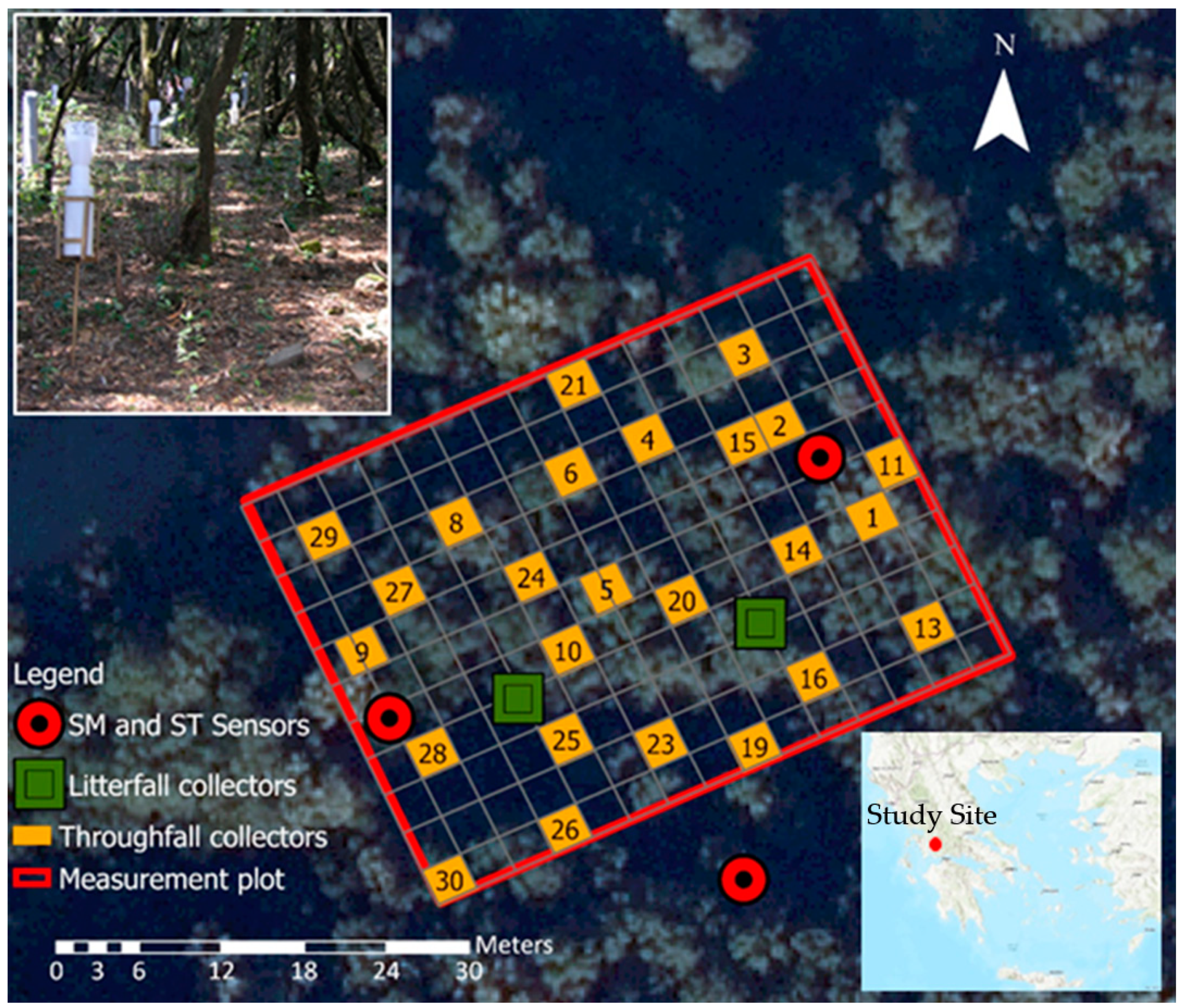
2.1. Study Area

The study was carried out in a forest plot (45 m × 33 m) located in western Greece (38°50′46″ N, 21°18′16″ E, alt: 340 m a.s.l.) as shown in Figure 1. The dominant tree species of the plot is Quercus ilex, and the sub-floor hosts mainly Arbutus unedo, Phillyrea latifolia and Erica arborea shrub species. The herbaceous floor and its composition with hygrophyte and mesohygrophyte species (Smilax aspera, Asplenium trichomanes, Asplenium onopteris, Asplenium adiantum nigrum, Carex distachya, Selaginella denticulate) and moss (Scleropodium purum) confirm the exceedance of 1000 mm annual rainfall in the area. This floor is not particularly dense but becoming denser in the gaps of shrubs and on their edges; its coverage can seasonally (mainly in spring) exceed 90% of the ground. In general, the evergreen broadleaved species are dense, presenting a LAI = 5.8 and height ranging from 6 to 15 m. The parental soil material is flysch and the soil type is Eutric Cambisol [46].

The climate of the area is warm temperate with hot and dry summers, classified in type Csa according to the modified Köppen–Geiger world map classification [47]. Based on UNEP’s [48] aridity climate classification, the climate of the broader area is humid [49] presenting a Thornthwaite’s [50] aridity index value of 0.78 during the recent climatic period (1960–1997). This is significantly decreased compared to the previous period (1930–1960) when its value was 0.85, indicating a rapid local climate transition to more arid conditions [41]. According to the data from the meteorological station installed in a forest opening near the plot (420 m) covering the period from 1973 to 2020, the average annual air temperature is 15.4 ± 0.64 °C, varying seasonally from 7.4 ± 1.37 °C in winter to 23.9 ± 1.38 °C in summer. The precipitation has an average annual value of 1049 ± 225.5 mm and presents what is expected for the Mediterranean climate seasonal variation: unevenly distributed between seasons with higher amounts falling in winter (40.2%) and autumn (33.3%). The pluviothermic diagram in Figure 2 confirms a water deficit period of about of 3 months starting from June until the beginning of September.

2.2. Data Collection and Processing

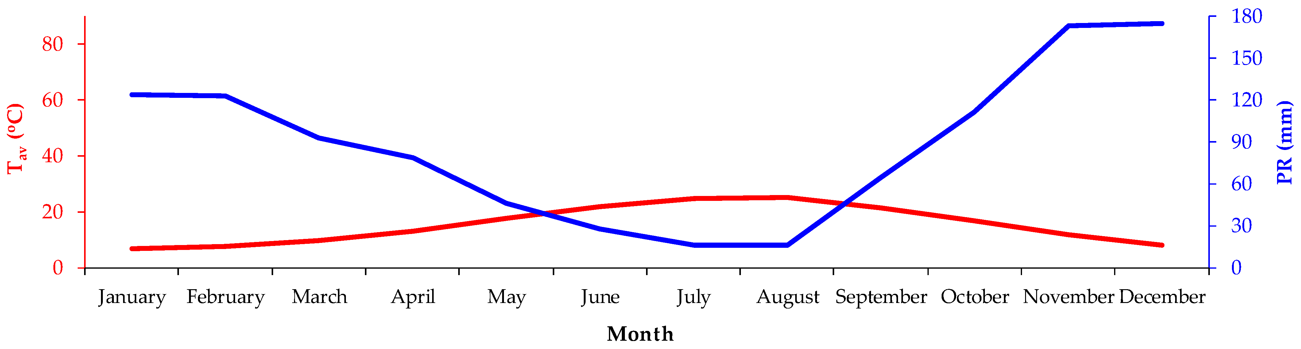
2.2.1. Air Temperature and Precipitation Data

Air temperature was recorded with a time step of 15 min for a 6-year period from 1 January 2013 to 31 December 2018 inside the meteorological station using an MP101A-T7-WAW sensor (Rotronic Measurement Solutions). The monitoring of the air temperature was continuous, and there were gaps only for 68 days due to malfunction of the sensor (3.1%). There was no gap filling, and the gaps were excluded from the analysis.

Bulk precipitation (PR) was measured by a Belford rain gauge installed in the above-mentioned forest opening with its orifice at a height of 1.5 m above ground. Its recording tapes can continuously measure PR up to a maximum of 300 mm. The intensity of each rainfall event was analysed in an hourly time step from the readings of the recording tapes. Individual rainfall events were defined assuming that there was at least a six-hour interval with zero rain between them. The volume of measured PR (mm) was also compared with the average volume collected from three volumetric gauges installed next to the Belford rain gauge at the same height.

Two different flows are essential for the investigation of SM temporal variation: throughfall precipitation, which is the amount of PR water that penetrates the forest canopy, and stemflow, which is the flow from PR that drains down the trunks of trees. The sum of these flows constitutes the effective rainfall (PR_ef) that reaches the ground and is responsible for the formation of SM.

For the measurement of throughfall, a 25-volumetric collector network installed under the forest canopy (Figure 1), following the reports of Rodrigo and Avila [51] and Llorens and Domingo [52], was used. The collectors’ orifices were at 1.30 m above soil surface, and they were vertically adjusted regardless of the topographical slope. Effective rainfall (PR_ef) daily values were estimated as the sum of throughfall and stemflow, assuming that throughfall is produced in rainfall events with PR > 4 mm, except for the cases where the small rainfall events occurred on consecutive days, as suggested by Baloutsos et al. [53,54] for the same site. The authors [53,54] also proposed the following equation for the estimation of daily stemflow for the rainfall events with PR > 10 mm:

$$\mathrm{Stemflow}=\{\begin{array}{c}0.0934 \mathrm{PR}-0.7299 \left(\mathrm{March} \mathrm{to} \mathrm{August}\right)\\ 0.1064 \mathrm{PR}-1.2416 \left(\mathrm{September} \mathrm{to} \mathrm{February}\right)\end{array}$$

(1)

2.2.2. Soil Moisture and Soil Temperature Data

SM and ST data were recorded every hour in three representative plot replicates (Figure 1) at four soil depths (−5, −20, −40, −70 cm) using ECH2O EC-5TM water content and temperature sensors (Decagon Devices Inc., Pullman, WA, USA), with an accuracy of ±1 °C for ST and ±0.03 m³/m³ or ±3% VWC for SM, using the Topp equation which is typical in mineral soils with solution electrical conductivity lower than 10 dS/m. For this study, no additional sensor calibration was performed considering adequate data quality, since for all soil samples the electrical conductivity was lower than the above mentioned threshold. However, it should be mentioned that the vicinity of the sensors to roots and stones, as well as the carbon content of the soil, may have an impact on the quality of measurements, though this impact was considered to be systematic. In this work, SM and ST are used as indicative parameters to assess vegetation water stress. The triplicate design for the network of sensors adopted in this study is considered appropriate for monitoring the variability of SM and ST at different depths and seasons [55]. After the installation of the sensors, we allowed a four-month wet period (September to December 2012) for the stabilization of the measurements and to identify any quality issues. The daily values of SM and ST were calculated as averages from the hourly data. In this work, the annual SM and ST profile patterns were also employed, and they were produced by the application of SURFER 13.6.618 software (Golden Software, LLC, 2016) using the kriging interpolating technique which estimates the unknown values at all points of a defined spatial domain using a weighted average of all known values around the unknown point [56].

2.2.3. Soil Sampling and Analysis

The soil sample collection was carried out by means of systematic sampling, following the guidelines suggested by the soil expert panel of the ICP Forests (http://icp-forests.net) (accessed on 13 February 2023) into which our experimental site is integrated and in the framework of project “Biosoil”. Inside the plot, along three 25 m long transects 5 m apart, six soil pits were excavated 5 m apart from each other on each transect. The organic horizons, comprising litter (L) and the fragmented horizon (FH) layers, were collected from each pit by means of a metallic frame having an area of 15 × 15 cm. Mineral soil layers were collected with a shovel from depths 0–10 cm, 10–20 cm, 20–40 cm and 40–80 cm. From a total of 18 soil samples, six (approximately 2 kg each) per horizon and soil depth were mixed to have three pooled samples per horizon and depth. The bulk density of the mineral soils was measured with a cylinder of known volume (129 cm³). The value was converted to bulk density of fine earth (<2 mm) after subtracting the volume of coarse material (stones and gravel). The percentage of large stones was estimated visually in the field. All soil samples were transferred to the laboratory and were air-dried. Apart from the L layer, the other samples passed through a 2 mm sieve. After the analysis, the samples were dried at 105 °C for 24 h, and the results were expressed in dry weight of soil at that temperature.

The soil–water retention curve (pF) and hydraulic conductivity function K(θ) were produced for the assessment of the soil hydraulic characteristics. Soil samples were taken during the installation of the SM and ST probes at the three measurement points (Figure 1) at depths of −20, −40 and −70 cm. Two samples were extracted per depth, resulting in a total number of 18 samples that were analysed in the laboratory. In total, 7 points of the pF curve were estimated from laboratory measurements using the method of the sand–kaolin box (following the protocol ISO 11274) for pressure heads down to −330 hPa and 5 more points for even smaller pressure heads using a pressure membrane apparatus (down to −5000 hPa). The 12 experimental pressure points were calibrated and verified by using the RETC software version 6.02 (©2005–2009) for the pF curve fitting. The remaining 6 samples were used for the results cross-validation.

To determine the hydraulic conductivity in saturation (K_s), the double-ring infiltrometer method was employed and 9 in situ experiments (3 on each measurement point) were conducted. The K_s was found to have an average value of 4.5 cm/h which is considered moderately high [57]. This value was imported in RETC for the prediction of the K(θ) curve along with the Van Genucthen–Mualem [58] parameters.

The texture analysis was completed using the hydrometer method [59]. The pH was measured electrometrically (pH meter ORION 410-A) using a glass electrode in water and 0.01 M CaCl₂ (1:5 soil weight per volume of water and CaCl₂ solution). The concentrations of total N and organic C in soils were measured with a CN analyser (Vario MAX) [60].

3. Results and Discussion

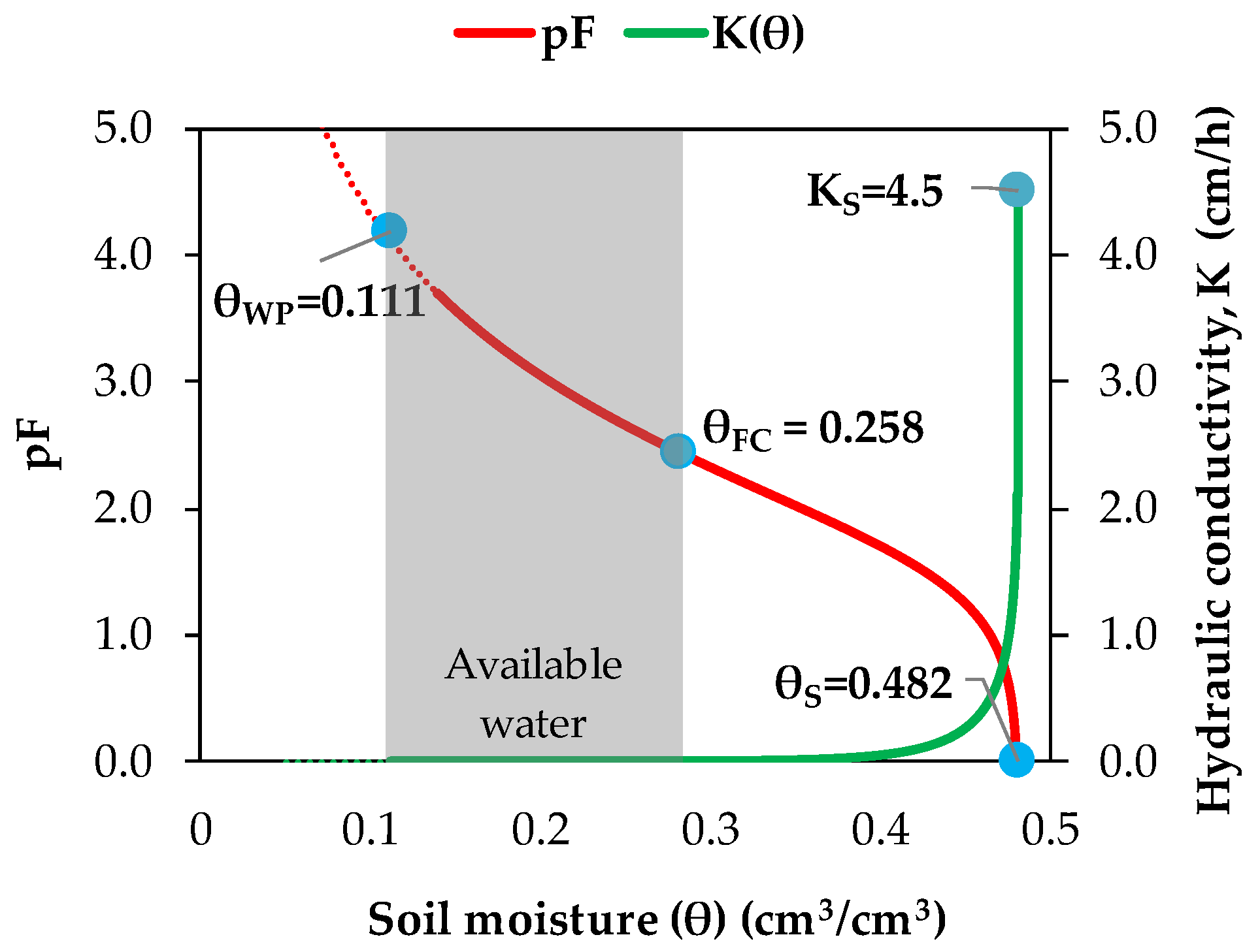
3.1. Soil Texture, Nutrient Status and Soil Hydraulic Properties

The soil is silty loam, and its reaction is slightly acidic (

Table 1. Average values of texture fractions (%), pH and concentrations of C and Ν (g/kg). Values of coefficient of variations (%) are shown inside parenthesis.

Soil layer	Clay	Silt	Sand	pH (CaCl2)	C (g/kg)	N (g/kg)	C/N
L					494.3 (2.84)	11.2 (8.46)	44.3 (11.18)
FH				6.09	259.7	13.6	19.1
				(1.82)	(7.13)	(8.19)	(1.39)
0–10 cm	23.63	56.07	20.30	5.60	49.5	3.0	16.3
	(6.24)	(2.41)	(8.91)	(1.15)	(13.98)	(13.39)	(2.21)
10–20 cm	24.20	54.23	21.57	5.43	27.3	1.9	14.4
	(14.48)	(0.56)	(14.85)	(7.81)	(16.74)	(13.73)	(3.61)
20–40 cm	25.97	52.83	21.20	5.26	14.4	1.2	12.5
	(15.81)	(1.52)	(21.56)	(2.52)	(17.19)	(14.37)	(3.34)
40–80 cm	29.27	50.67	20.07	5.71	8.6	0.8	10.4
	(15.18)	(4.90)	(21.64)	(10.56)	(14.48)	(11.00)	(5.45)

). The coefficients of variation (CV—defined as percentage of standard deviation over the mean) given in the parentheses of Table 1 show a small spatial variation (<15%) for all soil properties [61]. Moderate spatial variation exists only in 20–40 cm (21.56%) and 40–80 cm (21.64%) layers for the sand texture fraction, which does not affect the texture class (silty loam) at any measurement point [62]. According to B.A.I. [63], the nitrogen and organic carbon concentrations are satisfactory for plant demands. The ratio C/N is rather high in the litter (L) layer, but it goes down abruptly in the FH and mineral layers. This means that the decomposition rates are satisfactory. Michopoulos et al. [64] found that the soil organic matter in the maquis plot under consideration had a higher decomposition rate than that in a mountain fir forest in central Greece despite the fact that the fir forest had higher SM but lower ST. This suggests that ST is more important than SM regarding microbial activity when comparing different ecosystems.

Soil hydraulic behaviour is important for the assessment of soil–plant–atmosphere relations. The soil water availability and the water retention in soil profile are critical for plants and for the design and implementation of adaptation strategies to mitigate the impacts of climate change, especially in natural ecosystems. The soil water retention pF (fitted and extrapolated), the hydraulic conductivity K(θ) (predicted) curves derived from RETC software (R² = 0.995) and the main hydraulic characteristics are presented in Figure 3. Important values for the pF curve are SMs in field capacity (θ_FC = 0.258 cm³/cm³, pF = 2.525), in wilting point (θ_WP = 0.111 cm³/cm³, pF = 4.18) and in saturation (θ_s = 0.482 cm³/cm³). According to these values, the soil profile down to −70 cm can potentially hold 337.0 mm of water in saturation conditions, which is much greater than the amount of water available for vegetation (102.9 mm). It should also be stated that the fitted residual water content (θ_r) is in line with the findings of Dexter and Richard [65] who reported that the amount of adsorbed water on soil particle surfaces is zero at pF = 6.6. The resulting Van Genuchten parameters from the application of RETC, for the pF curve and their standard error, are a = 0.0260 ± 0.0023, n = 1.2777 ± 0.0105 and m = 0.2174. The results of the prediction of the K(θ) curve (green line) show, as expected, that K is decreasing very abruptly from K_s (4.5 cm/h) to the value of Κ = 0.05 cm/h (θ = 0.400 cm³/cm³) which results in extreme small velocities.

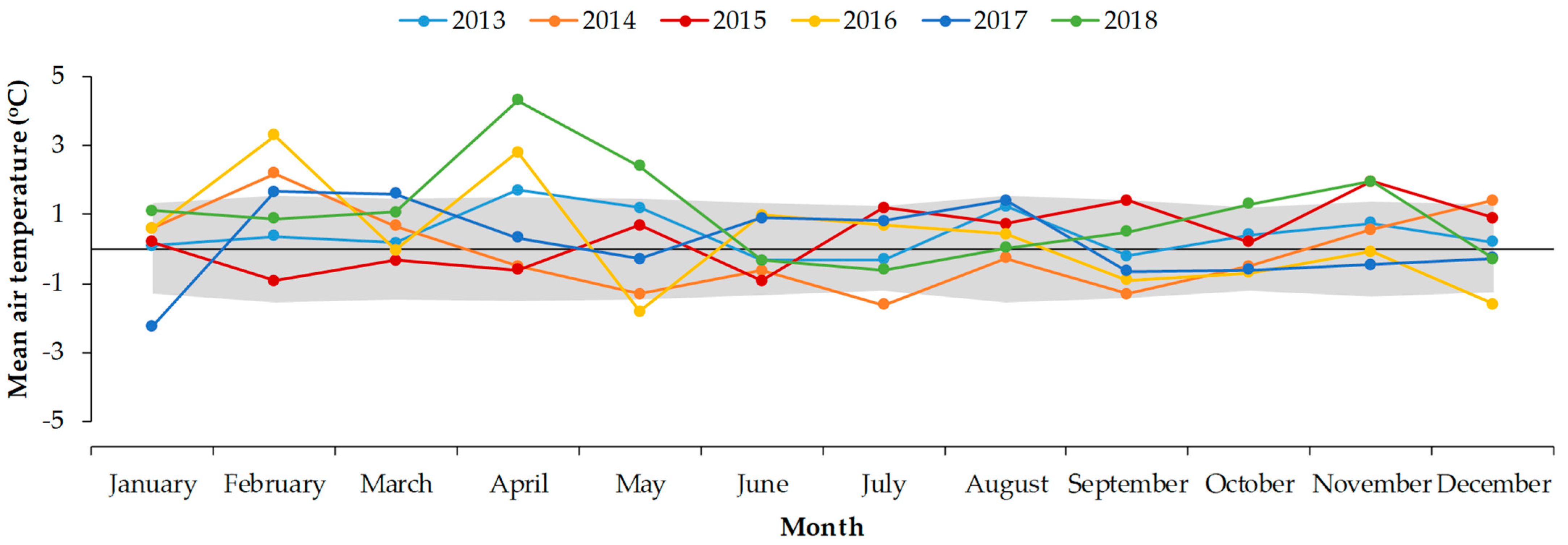
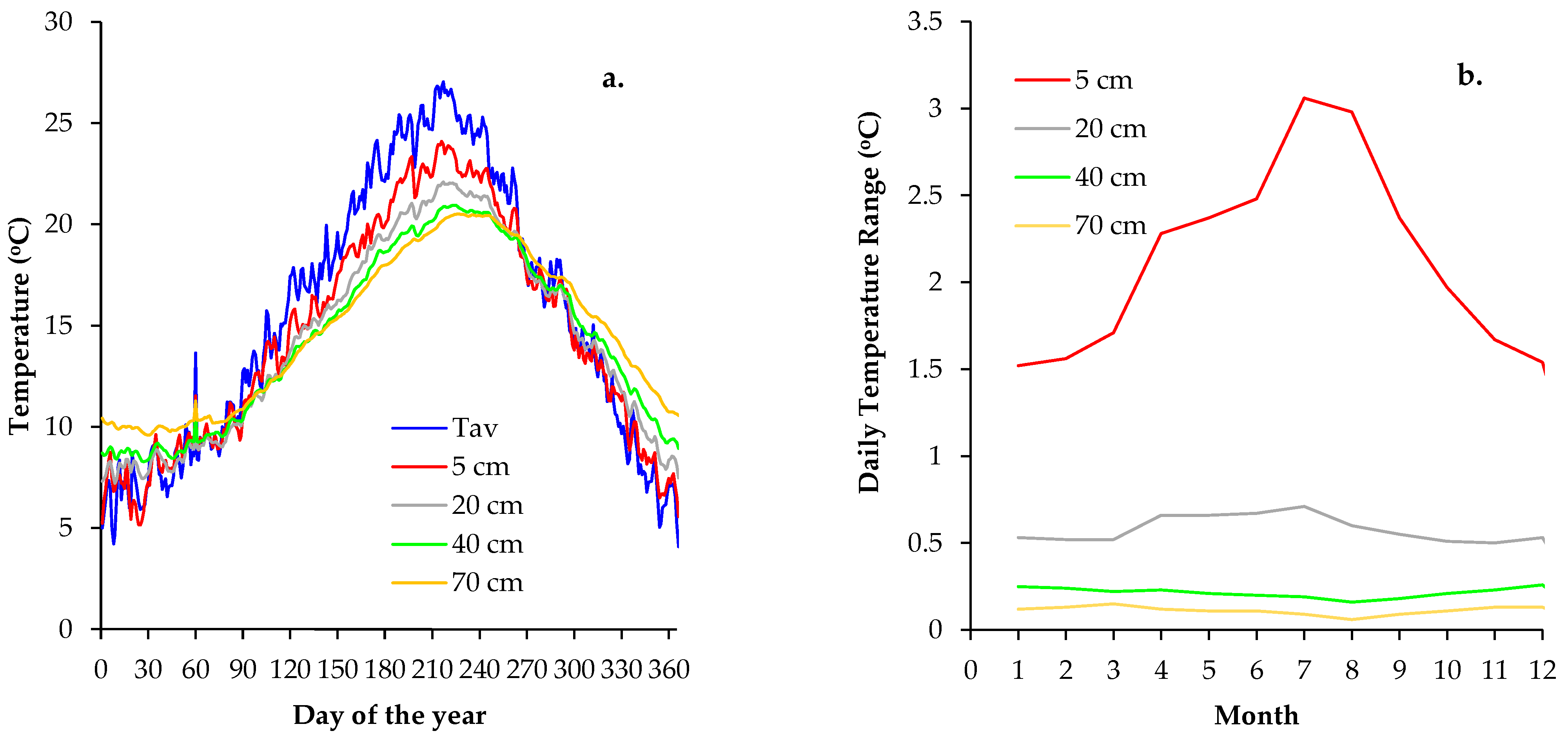
3.2. Temporal Variations of Air Temperature

The annual average air temperature (T_av) for the 6-year study (15.7 °C) is quite similar with its long-term respective value for the climatic period 1973–2020 (15.4 °C), ranging on an inter-annual basis from 15.3 °C in 2014 to 16.4 °C in 2018. The air temperature variability is even more sound monthly, and specific months were much warmer or cooler from what was expected based on the climatic profile of the region. The deviations from the local long-term climatic mean for every month are depicted in Figure 4 along with the standard deviations (SD) of the monthly T_av of the 1973–2020 climatic period.

Results indicate that all monthly air temperatures of the years 2013 and 2015 are within the limit value chosen by the authors of “mean ± 1SD” from the climatic means, suggesting normal meteorological conditions in terms of temperature. Similarly, the year 2014 had the expected monthly temperatures for all months, except for February, when slightly warmer conditions (by +2.2 °C) prevailed. In 2016, February and April were also warmer (by +3.3 and +2.8 °C, respectively), whereas in 2017, January temperatures were cooler (by −2.2 °C). Finally, in 2018, April, May and November temperatures have exceeded the climatic normal by +4.3, +2.4 and 2.0 °C, respectively. The above pattern indicates that during our study period the temperatures of the environment were rather normal for the area and in some cases warmer.

The general intra-annual pattern of temperature is coherent with the typical distribution of the Mediterranean climate presenting seasonal variability: higher values in summer (+24.1 ± 0.84 °C), lower in winter (+7.9 ± 1.23 °C) and intermediate values of +14.3 ± 1.42 °C and +16.6 ± 0.93 °C for the transitional seasons of spring and autumn, respectively (

Table 2. Monthly T_av, average monthly PR and PR_ef (mm) for the study period 2013–2018.

Month	Tav			PR			PRef
	Values (°C)	SD (mm)	CV (%)	Volume (mm)	SD (mm)	CV (%)	Volume (mm)	SD (mm)	CV (%)
January	6.9	1.2	17.2	210.9	73.9	35.0	152.8	54.8	35.9
February	8.7	1.5	16.9	196.9	121.9	61.9	139.8	100.5	71.9
March	10.4	0.7	7.0	147.7	60.5	41.0	106.5	49.2	46.2
April	14.4	2.0	13.6	61.8	63.5	102.8	38.9	41.5	106.8
May	18.0	1.6	8.8	75.8	68.6	90.5	56.1	57.6	102.7
June	21.8	0.8	3.7	49.5	36.7	74.1	34.1	28.1	82.5
July	24.8	1.1	4.3	7.1	7.6	107.0	3.5	3.9	110.5
August	25.7	0.7	2.6	6.0	13.0	216.7	4.7	10.5	222.9
September	21.0	1.0	4.7	86.2	87.5	101.5	60.8	65.9	108.3
October	16.8	0.8	4.6	96.6	75.7	87.8	69.8	62.8	90.0
November	12.5	1.0	8.0	220.5	84.4	38.2	176.0	76.2	43.3
December	8.1	1.1	13.0	141.3	172.9	122.4	106.9	138.9	129.9

). The warmest month is August (25.7 ± 0.66 °C) and the coolest is January (6.9 ± 1.18 °C).

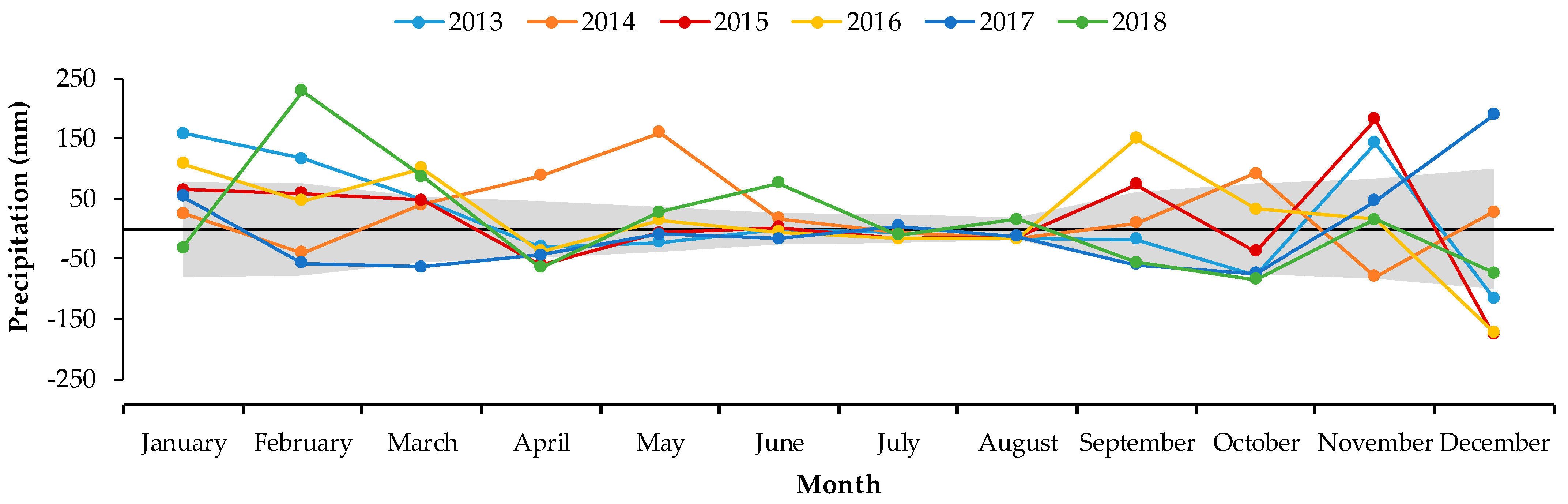
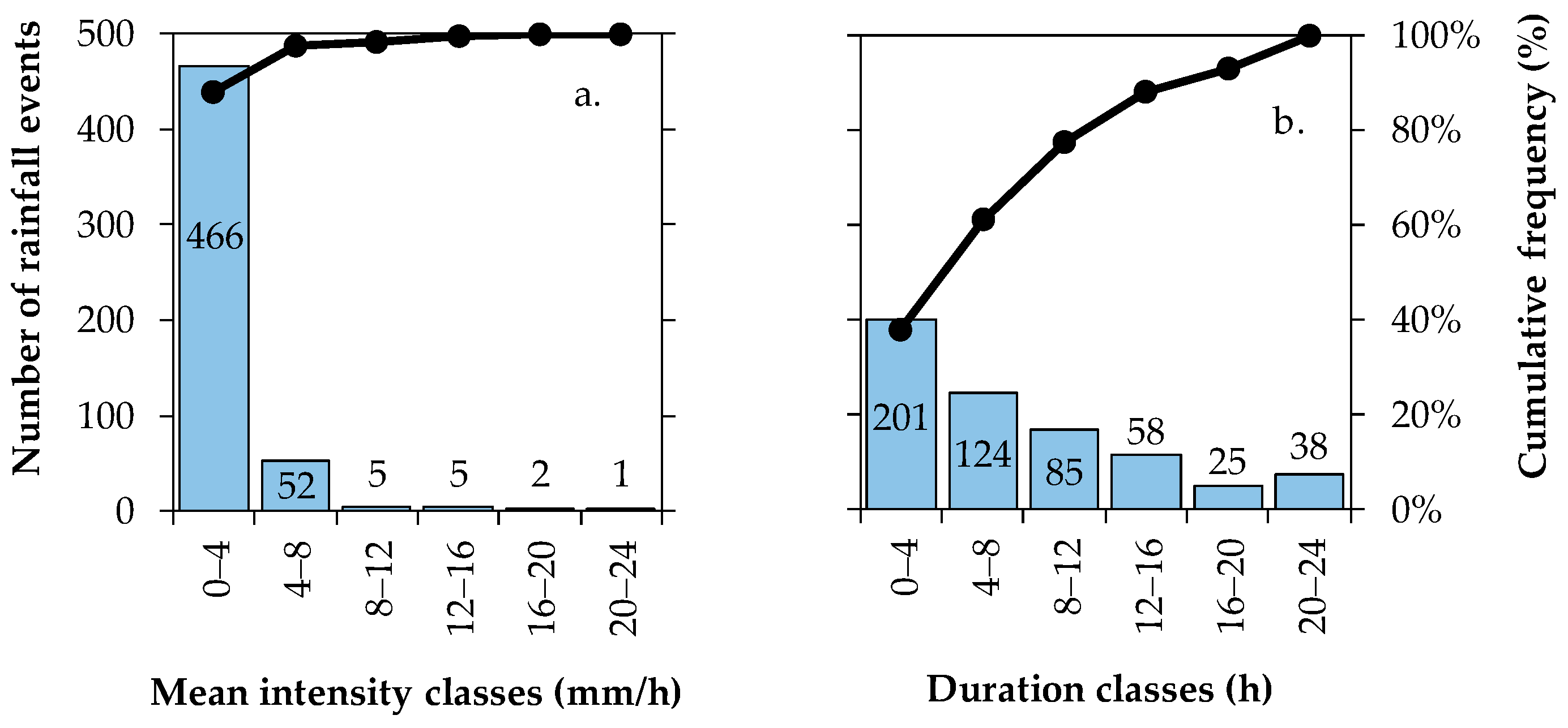
3.3. Precipitation Variations and Characteristics

The total rainfall events that occurred in the 6-year period of the study were 531. Annual PR ranged from 1090.4 mm in 2017 to 1525.0 mm in 2014, suggesting that all years of the study are wetter compared to the long-term annual PR average of the 1973–2020 period (1049 mm) with percentages ranging from +4% in 2017 to +45% in 2014. The monthly PR values during the study period (2013–2018) showed that November was the wettest month of the year (221 mm) and August the driest one (6 mm). In general, the annual PR yield mainly occurred in winter (549 mm) and autumn (403 mm), and to a lower degree, in spring (285 mm) and summer (63 mm).

The monthly PR deviations from the respective long-term means are shown in Figure 5, along with the SD of the monthly PR of the 1973–2020 climatic period. In 2013, January (+128.3%), February (+95.0%) and November (+82.9%) received higher and December (−65.7%) lower amounts of PR since their respective PR values are out of the threshold of “mean PR ± 1SD”. In 2014, only wetter months were recorded, and these were April (+113.1%), May (+344.6%) and October (+82.7%), whereas in 2015, September (+112.5%) and November (+105.5%) were wetter and April (−75.2%) and December (no rain) drier. In 2016, January (+87.2%), September (+231.1%) and March (+109.1%) had a higher PR and December (no rain) a lower one. Finally, December 2017 (+107.9%) and February (+186.3%), March (+94.0%) and June (+272.3%) 2018 were wetter, while March (−67.7%) 2017 and April (−82.2) 2018 were drier. An increase in rainfall variability is one of the key findings of all anthropogenic scenarios in global climate model projections [66,67]. Our results indicate a high monthly variability in PR which is consistent with the findings of other studies implemented in the Mediterranean [35,68]. The above mentioned percentages refer to the percentage differences from the respective monthly climatic PR of the period 1973–2020.

To investigate the rainfall characteristics, the 531 rainfall events that occurred during the study period were grouped into categories based on their mean intensity and duration (Figure 6). The great majority (87.8%) of the incidents was of low intensity (<4 mm/h). These are associated with 74.4% of the total PR, and their low intensity enhances the ability of the soil to store water in the root zone and/or to infiltrate water deeper. The extreme intense rainfall events are rather scarce, considering that in our 6-year study only 13 incidents were recorded with an average intensity greater than 8 mm/h and only one of these had an intensity higher than 20 mm/h. The 13 relatively high-intensity rainfall events accumulated only 5.2% of the incoming total PR in the ecosystem, and 10 of them had small durations (<4 h) that could result in risks to the forest soil matrix (erosion or increased runoff).

Regarding event duration, in most cases (62%) rainfall lasts more than 4 h. For the rest of the events (duration with less than 4 h), it should be mentioned that, in general, they provided 15.4% of the total PR to the ecosystem and in most cases are characterized by low mean intensities (83.5% on average). The effective part of precipitation (PR_ef) also presents similar variability.

The average monthly PR_ef for the study period (Table 2) ranges from 3.5 ± 3.9 mm (49.3% of PR) in July to 176.0 ± 76.2 mm (79.8% of PR) in November. It is also perceived that the wettest month is November followed by January, while summer months August (6.0 mm) and July (7.1 mm) are the driest ones. Both monthly SD and coefficients of variation (CV) presented similar variations during the year in both PR and PR_ef. It is worth noting that extreme values of CV for August are due to the occurrence of only one rainfall event in 2017 (3.8 mm PR) and four rainfall events in 2018 (32.4 mm PR), while the other four years of observation no rainfall events occurred. In general, the annual PR_ef ranged in our study from 843.8 mm in 2017 to 1046.8 mm in 2014, representing 77.4% and 68.6% of PR, respectively. Similar percentages were also presented by other studies. Baloutsos et al. [69] measured PR_ef values of 68.0% ± 3.2% in the same forest plot for a seven-year period. Llorens et al. [10] measured a bulk interception of 24% of PR in a Pinus sylvestris forest patch in a Mediterranean mountainous area, which indicates that 76% is attributed to PR_ef. Avila and Rodrigo [70] estimated in two Quercus ilex stands in Spain PR_ef percentages of 79.1% and 77.5%, respectively. Vicente et al. [36] simulated PR_ef values in four mixed Mediterranean forests in Spain which ranged from 56.8% to 75.9% of PR.

In the forest environment, the complex interactions between the canopy and rainfall characteristics determine the throughfall inputs [71] and therefore the interception rates [8]. As rainwater drips through the forest canopy, the droplets’ diameter, velocity and kinetic energy change [8], thus introducing higher variability of the water distribution on the forest soil surface and highly affecting the soil’s moisture and temperature profiles as well as the soil’s infiltration properties, both spatially and temporally. In our study site, the kinetic energy of PR_ef (mainly THR) is expected to be small due to the rather dense canopy (LAI = 5.84) in conjunction with the rainfall events that are mainly of high duration and low intensity. This enhances the ecosystem’s ability to infiltrate water with higher rates and limits the possibility for surface runoff formation, even if hydraulic conductivity is relatively low.

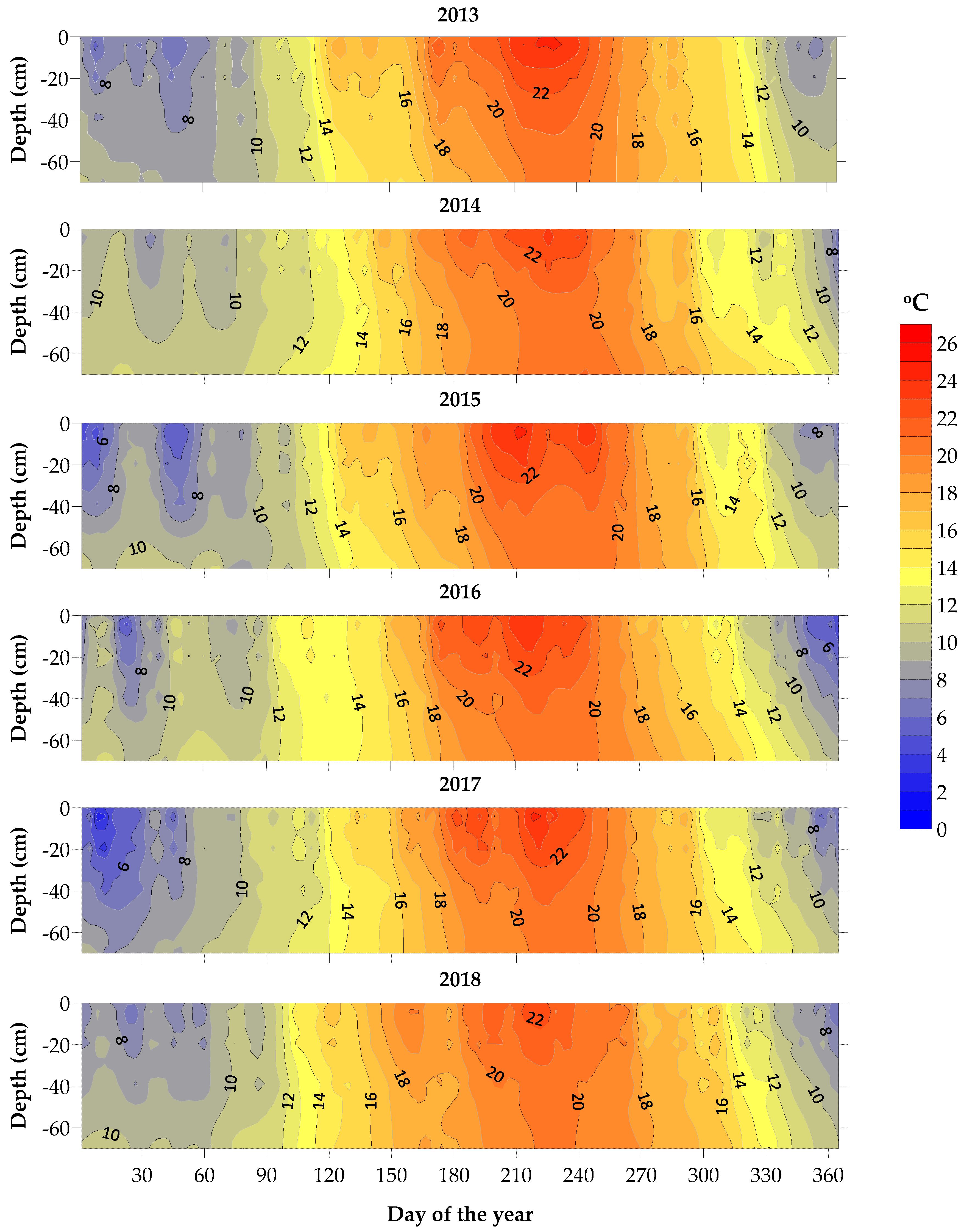
3.4. Temporal Variations of Soil Temperature

Annually, ST showed a mean value in −5 cm of 14.5 ± 1.64 °C, in −20 cm of 14.4 ± 1.30 °C, in −40 cm of 14.3 ± 0.99 °C and in −70 cm of 14.7 ± 0.87 °C. The general pattern of ST at all depths depicts the same distribution with air temperature (see Table 2, T_av), also presenting a seasonal variability with higher values in summer, lower in winter and intermediate values for the transitional seasons of spring and autumn (

Table 3. Soil temperature (ST) variations with depth for the period 2013–2018.

Month	ST (°C)				SD (°C)				CV (%)
	5 cm	20 cm	40 cm	70 cm	5 cm	20 cm	40 cm	70 cm	5 cm	20 cm	40 cm	70 cm
January	7.4	7.9	8.6	10.0	2.08	1.73	1.33	0.96	28.26	21.84	15.43	9.61
February	8.2	8.6	8.9	10.0	1.80	1.39	1.11	0.83	21.96	16.26	12.49	8.31
March	9.5	9.7	9.8	10.5	1.18	0.98	0.75	0.89	12.33	10.12	7.66	8.52
April	12.6	12.4	12.1	12.1	1.68	1.42	1.06	1.05	13.32	11.40	8.73	8.66
May	16.0	15.5	14.9	14.6	1.49	1.23	1.07	0.90	9.33	7.91	7.16	6.15
June	19.0	18.4	17.5	16.9	1.70	1.42	1.14	1.06	8.97	7.68	6.52	6.27
July	21.8	20.9	19.8	19.1	1.26	1.00	0.72	0.70	5.78	4.77	3.64	3.68
August	22.9	21.9	20.8	20.4	1.01	0.66	0.41	0.31	4.41	3.01	1.96	1.54
September	19.6	19.5	19.2	19.5	1.71	1.32	0.94	0.75	8.71	6.77	4.88	3.83
October	16.0	16.3	16.5	17.2	1.65	1.28	0.94	0.77	10.35	7.85	5.68	4.45
November	12.3	13.0	13.7	14.7	1.97	1.56	1.20	0.98	16.03	12.00	8.75	6.69
December	8.5	9.3	10.3	11.7	2.08	1.62	1.29	1.21	24.42	17.56	12.52	10.30

). Results from previous studies showed that ST memory increases with soil depth and varies seasonally [30,72].

Soil temperature memory varies with season, and deep soil layers have more significant seasonal differences than subsurface soil. The CV index showed a downward trend with depth but with a steeper decline up to the −40 cm. The ST varies inside the soil profile, presenting values with differences among the various depths that range from 0.4 ± 0.96 °C in September to 3.2 ± 0.87 °C in December. With respect to CV and depth, results show larger values in winter months (18.6% in January, 14.1% in December and 13.6% in February). Both SD and CV decrease their values with depth during all months; the warmest month is August with an ST range with depth 2.5 ± 0.60 °C, while the coolest one is January (range 2.6 ± 1.52 °C).

Figure 7a illustrates the mean daily time of ST at four different depths (−5 cm, −20 cm, −40 cm and −70 cm) along with the mean daily T_av for the study period. Compared to T_av, the soil profile is warmer in the lower depths at the beginning of the year (January, February). It is notable that the diurnal range of ST is highly variable with depth, presenting high diurnal changes at the topsoil zone that rapidly decrease with depth, as is clearly depicted in Figure 7b. The rather stable ST throughout the 24 h day period is mainly observed for the −40 cm and −70 cm soil zones regardless of the season, whereas at the upper soil layers (−5 cm and −20 cm) the diurnal ST ranges maximize in summer.

In March, the temperature differences between T_av and the four sensors (at four depths) decrease and tend to equalize; hence, the soil profile shows the same ST throughout its depth which is similar with T_av. However, for a few days (during April), the temperature profile reverses, presenting higher values in the surface that decrease with depth. During this period, the differences between T_av and STs become positive and maximized in August, decreasing thereafter until the end of September when all STs and T_av become equal. By October, the ST profile reverses again and for the next months until the end of February the soil is warmer when compared with the air above, and ST increases with depth in the soil profile. In general, the decreasing rate of ST with depth in winter is about 0.036 °C/cm, whereas in summer the respective rate is of the same magnitude (0.035 °C/cm) but decreasing.

August is the month when the smallest SD and CV values of ST in −70 cm appeared. This strengthens the conclusion that the lack of precipitation and the high temperatures for this month stabilize ST values in the soil profile [72]. Thus, until the beginning of September, ST shows its greatest values, as expected, at −5 cm and then at −20 cm, −40 cm and −70 cm. In September and until the end of the year, the shape of ST in the soil profile shows the shape it had in the first two months of the year. Regarding the fluctuations of ST with soil depth, results show high values at the depth of −5 cm and gradually smoothing out from −20 cm to −70 cm where ST fluctuations are very small. The results clearly show that ST is affected by T_av at different depths, but less so as depth increases. This is due to the stronger persistence effects that prevail in the deeper soil layers originating from previous conditions. According to Bilgili [73], these ST reversals are very important, especially during the winter period, as they generate soil biological activities. Zhang et al. [30] found a significant impact of air temperature on the ST values of the shallower soil layers. Finally, compared to daily T_av, the whole soil profile has a higher temperature from the beginning of the year until March and from October until the end of the year.

The simulation in Figure 8 confirms the temporal variation in ST. The values of ST at least at the depth of −5 cm were clearly affected more intensely by air temperature. However, the rates of change both on a daily and annual basis are noticeably smaller compared to T_av.

The simulation also confirms the finding that the largest ST variation occurs up to the depth of about 40 cm. According to Terradas and Save [39], transpiration rates showed a linear significant decline with decreasing soil temperature, and Lloyd and Taylor [27] found that the effective activation energy for respiration varies inversely with T_av. Combining these findings with our results we can conclude that respiration rates are higher in the upper layers, independently from the root mass. Nevertheless, this is a case for further investigation. Even though the shading of the soil due to the presence of vegetation is strong (LAI = 5.84), at least in the first 20 cm the temperature response is significantly affected.

Until the end of March, the temperature of the soil profile does not exceed 12.0 °C. The transitional period of the quarter April–June presents many fluctuations in the soil temperature values, both in relation to depth and over time. Indicatively, year 2013 shows from the beginning of April until the middle of May a higher temperature by at least 1.0 °C in the first 25–30 cm compared to the lowest depths. Meanwhile, the year 2016 shows from the beginning of April until the middle of June a gradual increase in ST with approximately parallel lines for the entire soil profile. Despite all the different daily fluctuations, the temperature of the soil profile does not exceed, at the end of June in any year, 20.0 °C, except in the upper layers (up to −20 cm) in 2013, 2014, 2016 and 2017, presenting within this quarter an increase of approximately 8.0 °C.

Within the next quarter (July–September), for all years, the temperature rises to 24.0–25.0 °C, showing again the pattern of the first months of the year, i.e., only up to the depth of the first 40 cm. ST in the last 30 cm depth exceeded 20 °C in all years only for the very hot period from the beginning of August until the first days of September. By the end of September, the ST of the whole profile decreases to 18.0 °C with different rates at different depths for all years.

In the last quarter of each year, a gradual decrease in ST is observed throughout the profile. The strong variation in all years that appears from mid-November to mid-March, in the first 30–40 cm is mainly due to the occurrence of many PR rainfall events and the significant and rapid temporal storage of water in the soil. The same strong variation appears during the summer period when the high values of air temperature influence the ST values.

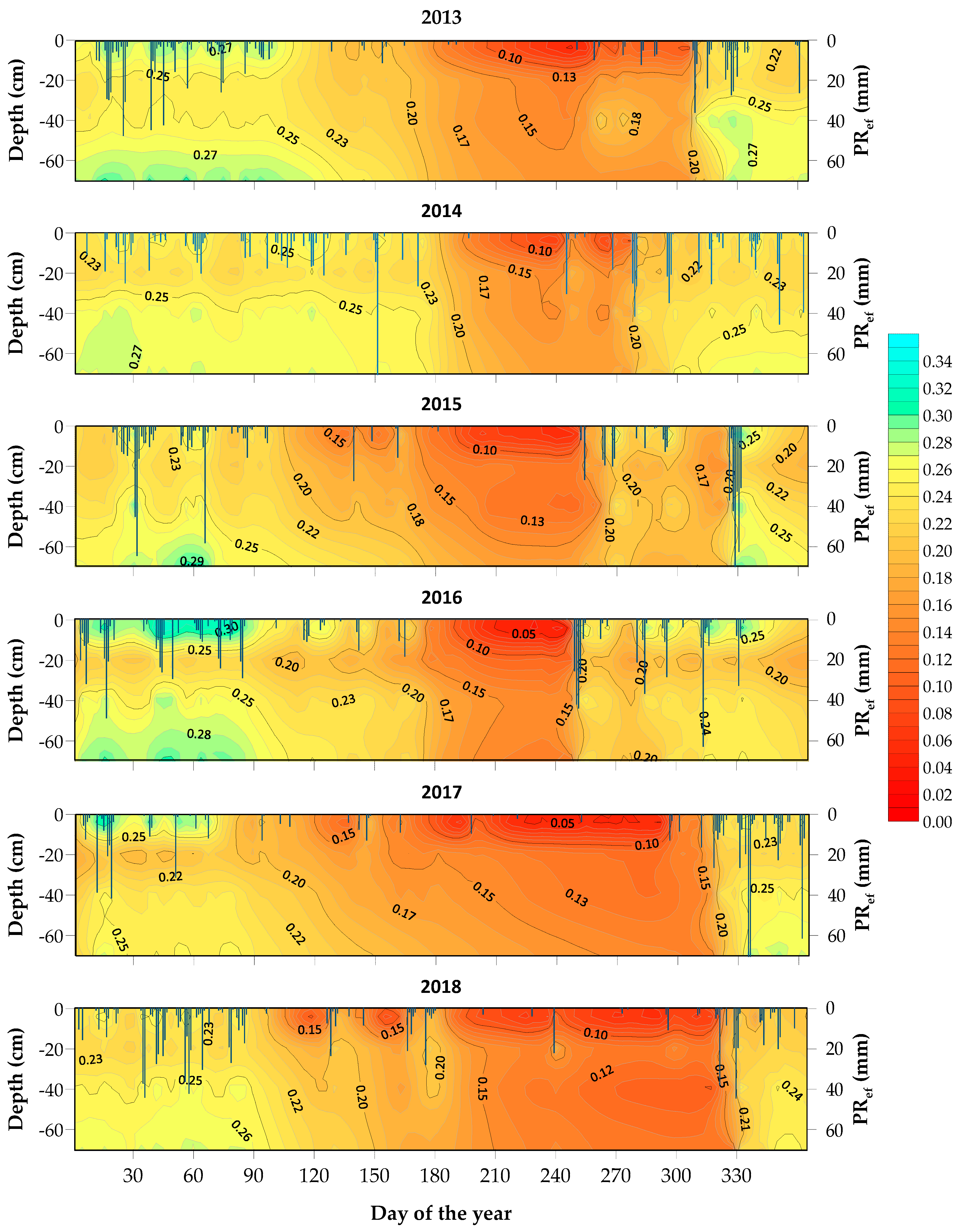
3.5. Temporal Variations in Soil Moisture

The results for the whole study period in monthly values are presented in

Table 4. Soil moisture (SM) variations with depth for the period 2013–2018.

Month	SM (cm3/cm3)				SD (cm3/cm3)				CV (%)
	5 cm	20 cm	40 cm	70 cm	5 cm	20 cm	40 cm	70 cm	5 cm	20 cm	40 cm	70 cm
January	0.257	0.221	0.251	0.271	0.032	0.017	0.018	0.017	12.2	7.9	7.5	6.2
February	0.268	0.224	0.253	0.275	0.030	0.017	0.016	0.018	11.2	7.7	6.3	6.4
March	0.254	0.224	0.250	0.271	0.037	0.015	0.015	0.017	14.5	6.6	6.2	6.3
April	0.215	0.211	0.233	0.254	0.048	0.020	0.019	0.019	22.4	9.7	8.4	7.3
May	0.186	0.196	0.214	0.234	0.051	0.022	0.026	0.021	27.5	11.1	11.1	8.8
June	0.168	0.179	0.198	0.211	0.047	0.029	0.031	0.026	28.3	16.4	15.8	12.4
July	0.102	0.153	0.162	0.174	0.033	0.022	0.019	0.018	32.6	14.8	11.7	10.4
August	0.065	0.136	0.139	0.156	0.018	0.015	0.012	0.013	29.0	11.3	8.7	8.3
September	0.115	0.152	0.159	0.165	0.077	0.029	0.044	0.030	66.5	19.1	28.1	18.1
October	0.152	0.166	0.177	0.172	0.080	0.032	0.051	0.037	52.8	19.5	28.8	21.5
November	0.209	0.193	0.213	0.212	0.066	0.035	0.058	0.054	31.7	18.2	27.3	25.4
December	0.229	0.212	0.243	0.260	0.025	0.017	0.017	0.016	10.9	8.1	6.9	6.2

. Overall, annual SM at −5 cm had a mean value 0.185 ± 0.203 cm³/cm³; at −20 cm 0.174 ± 0.205 cm³/cm³; at −40 cm 0.208 ± 0.114 cm³/cm³; and at −70 cm 0.221± 0.119 cm³/cm³.

Seasonal variability was also observed with higher values in winter (0.247 ± 0.020), lower ones in summer (0.154 ± 0.024) and intermediate values in spring (0.229 ± 0.026) and autumn (0.174 ± 0.049) (Table 4). Spring is the crucial season during which water needs are high for tree growth and determines the duration and the severity of water stress [37]. According to Barbeta et al. [31], maquis vegetation with dominant species such as Quercus ilex, Arbutus unedo and Phillyrea latifolia form a dimorphic root system, which has the ability to differentiate soil water uptake, depending on the soil moisture content. Therefore, vegetation adapts to the prevailing meteorological conditions, thus shaping water absorbing conditions at different depths. This could be the reason that explains decreasing SM values (due to hydraulic decrease) during the transitional spring season. Additionally, it could be attributed to the fact that quick drainage may promote aeration in surface soil, hence optimizing the occurred conditions in the upper layers’ roots [74].

The monthly CV displays, according to depth (0–70 cm), a range from 48.4% in September and 31.3% in October to 4.7% in December and 4.8% in February. This is because the dry soil profile is moistened with the water of autumn’s rainfall events but at rates inextricably linked to their intensities which in our study are bigger during the autumn months (2.6 and 2.3 mm/h, respectively) than in the winter (both 2.0 mm/h) ones. Overall, the smallest values of CV at all depths are recorded in December for −5 cm (10.9%), in March for −20 cm (6.6%) and −40 cm (6.2%), and in January for −70 cm (6.2%). To the contrary, the highest CV values are recorded in the autumn months. This behaviour could be attributed to the fact that during the winter months the soil moisture has higher values due to many rainfall events, while during the autumn months, even though it rains, the infiltrated water mainly moistens the soil profile because this season follows the dry summer period [30]. Additionally, it has also been established from previous studies that the existence of more roots in the upper layers of the soil increase and decrease the soil’s moisture more intensely, while the lower layers are usually wetter, showing smaller variations in their soil moisture values [43,75].

During the period of June to early of September, vegetation is in water stress due to low PR values (<20 mm), higher ST values (>18 °C) and solar radiation, and therefore, gradually increased values of evapotranspiration. This situation leads of course to an increase in respiration rates, mainly due to an increase in decomposers’ respiration activity depending on their composition, litterfall amounts and quality [26,76]. This is very important because it is strongly establishing the relationship between carbon and nitrogen contents [77,78]. Hence, transpiration needs for tree vitality are served by water availability at lower depths, and therefore, SM values continuously decrease at all depths.

The seasonal SM variation indicated that, in general, drier conditions persisted in winter 2015 and 2018 and wetter ones in 2013, whereas spring of 2017 was the driest season and 2014 the wettest. During the critical summer periods of 2015, 2016, 2017 and 2018, dry conditions persisted, but the wettest summer was in 2014. In addition, autumn 2018 was the driest and the wettest in 2016. However, the above patterns varied highly with respect to soil depth.

The daily temporal variations in depth-wise soil moisture are presented in Figure 9 along with rainfall events, suggesting that SM in the upper soil zone (0–20 cm) presents high fluctuations and quick responses to PR [12,43], while in the −70 cm depth the range of the soil moisture is smaller and characterized by temporal stability with depth [79,80]. In general, the process of increasing moisture in the soil profile follows the distribution of PR. The prevailing low temperatures during the winter months and the occurrence of many rainfall events increase SM values. Nevertheless, the inclination of vertical isothermic curves (Figure 9) in spring varies, which leads us to the conclusion that the response in ST is very rapid down to 70 cm, while in SM, the response is slower mainly under 20 cm and could last until the beginning of the summer [45,74]. The SM and ST patterns are inversed during summer compared to winter, and the respective curves display similar but opposite inclinations. In autumn, following the dry summer period when SM minimizes, rainfall events impact highly on SM and ST, which present rapid responses. Their isolines become vertical, with similar SM and ST for the total soil profile (regardless of the soil depth), indicating that the soil profile is uniformly wetting and cooling. Such distribution is generally observed when the soil is rather dry and PR_ef amounts exceed 51.9 mm for 3–6 consecutive rainy days (e.g., 252–257 days of the year in 2016 and 321–327 days of the year in 2018).

Additionally, from the start of the growing season (April), a gradual decrease in SM values has been observed. This downward trend was interrupted only with the occurrence of precipitation [45,55]. It is worth noting that the lack of PR during the growing season (14 PR_ef rainfall events, 71.9 mm, 2.3 mm/h mean intensity) in 2017 formed a special water-stressed soil profile for vegetation’s needs from mid-April until late October. SM values at all depths for this period did not exceed 0.200 cm³/cm³ for at least 5.5 months (late May until late of November) during each monitoring year. Only in 2014, a very wet growing season (34 PR_ef rainfall events, 384.7 mm, 2.0 mm/h mean intensity) limited the water-stressed period to only 3 months (mid-June to early September) and with lower intensity (higher SM values). This situation indicates that the occurrence of rainfall events during the growing season is very important for the eco-hydrology of the study area since it increases water availability, and therefore, the capability of vegetation to overcome the dry summer season or an even larger drought period.

In terms of the water availability for the vegetation, daily SM values revealed that the whole soil profile is in general inside the range between field capacity (θ_FC) and wilting point (θ_WP) for all years. The results showed that during the wet semester, from October to March of the next year, daily SM values at the depth of −70 cm are above θ_FC which indicates the occurrence of soil water percolation. The percentages of these days are ranging from 71.4% (October 2013–March 2014) to 65.4% (October 2015–March 2016) but only 10.4% for the dry semester October 2017–March 2018). To the contrary, SM values at the depth of 5 cm from June to late September are below θ_WP, which indicates the important role of air temperature increase especially in the top layer of the soil profile.

The combination of phenological observations with the SM and ST patterns described above can enhance our knowledge about the vegetation’s behaviour. For example, in our study we detected that the magnitudes of SM were minimized (0.106 on average of all depths) in October 2018 compared to all other months of all years, indicating that the natural vegetation was facing strong water stress. Similarly, a low SM value was also recorded in October 2017 (0.115). The water stress and the warmer conditions, especially in 2018, have probably affected the flowering of Arbutus unedo that generally occurs in our site during October and November. Based on our phenological observations in 2017 and 2018, the beginning of flowering was delayed and started in December.

4. Conclusions

This study focuses on understanding the dynamics of soil moisture (SM) and soil temperature (ST) on a temporal basis in an experimental evergreen broadleaved mixed maquis plot in Greece by employing six years (2013–2018) of data for the continuous monitoring of the soil profile (0–70 cm) along with aerial meteorological attributes.

Air temperature influences more intensely the ST at the superficial soil depth (0–40 cm). Depth-wise ST changes are more pronounced in winter, when the average ST increases with depth, presenting a maximum difference of +2.5 °C at −70 cm compared to the superficial soil layer (0–5 cm). Of similar magnitude, though negative (−2.4 °C), is the respective ST difference in summer, indicating cooler soil conditions at greater depths. In contrast, the soil profile appears to be uniformly heated at all soil depths during spring, presenting negligible ST differences (indicatively −0.3 °C between −70 cm to 0 cm), whereas in autumn the soil profile pattern for ST is similar to winter but with smaller differences (maximum +1.2 °C between −70 cm to 0 cm).

The increase in SM is closely related to PR_ef. During the wet half of the year (October to March), SM at the upper soil layers (−5 cm, −20 cm) shows greater fluctuations compared to the rest of the year. In contrast, SM decreases continuously at all depths during the dry semester (April to September); this is due to the increased water demand of the vegetation and the correspondingly developed dimorphic root system. In spring, which is associated with the beginning of the growing season, the amount of precipitation could lead to limiting the length of the water stress period by up to 2.5 months, considering that summer precipitation in the region is generally scarce or not adequate to significantly increase the amounts of stored soil water in the root zone. This is very important for vegetation to be viable and sustain high growth rates. Before the beginning of the rainy season (in autumn), the soil profile presents minimum SM values (0.065 in August) quite lower than the wilting point (0.111). Thereafter, the impact of precipitation on the formation of the SM profile is critical. It was found that a period of three to six consecutive rainy days, with cumulative PR_ef greater than 51.9 mm, is sufficient to uniformly moisten the entire profile.

The above patterns of SM and ST are even more variable monthly, imposing the need for continuous monitoring of the soil profile. They also underline the importance of each of the time steps adopted for the analysis to produce reliable assessments of the effects of SM and ST on natural vegetation growth development and forest soil micrometeorological properties. The mean soil moisture content, computed for 6 years of the study period in the forest stand, was 0.201 cm³/cm³. This value and the value of 337.0 mm of water that the soil holds under saturated conditions indicate a sufficient potential for soil water storage to sustain local evergreen vegetation. In addition, the current study suggests that the SM and ST temporal variations may be useful tools for identifying the changes in phenology in rainfed ecosystems, especially in the Mediterranean region, but further research is required. In future work we will investigate the role of vegetation on the formation of SM and ST profiles in terms of their phenology and water requirements.

References

1. Berthet, L.; Andréassian, V.; Perrin, C.; Javelle, P. How crucial is it to account for the antecedent moisture conditions in flood forecasting? Comparison of event-based and continuous approaches on 178 catchments. Hydrol. Earth Syst. Sci. 2009, 13, 819–831. [Google Scholar] [CrossRef] [Green Version]
2. Peel, M.C.; McMahon, T.A. Historical development of rainfall-runoff modeling. Wiley Interdiscip. Rev. Water 2020, 7, e1471. [Google Scholar] [CrossRef]
3. Blöschl, G.; Bierkens, M.F.; Chambel, A.; Cudennec, C.; Destouni, G.; Fiori, A.; Kirchner, J.W.; McDonnell, J.J.; Savenije, H.H.; Sivapalan, M. Twenty-three unsolved problems in hydrology (UPH)—A community perspective. Hydrol. Sci. J. 2019, 64, 1141–1158. [Google Scholar] [CrossRef] [Green Version]
4. Vergarechea, M.; del Río, M.; Gordo, J.; Martín, R.; Cubero, D.; Calama, R. Spatio-temporal variation of natural regeneration in Pinus pinea and Pinus pinaster Mediterranean forests in Spain. Eur. J. For. Res. 2019, 138, 313–326. [Google Scholar] [CrossRef]
5. Bruijnzeel, L.A. Hydrological functions of tropical forests: Not seeing the soil for the trees? Agric. Ecosyst. Environ. 2004, 104, 185–228. [Google Scholar] [CrossRef]
6. Chen, S.; Wen, Z.; Jiang, H.; Zhao, Q.; Zhang, X.; Chen, Y. Temperature vegetation dryness index estimation of soil moisture under different tree species. Sustainability 2015, 7, 11401–11417. [Google Scholar] [CrossRef] [Green Version]
7. Wang, X.; Hao, Z.; Zhang, J.; Lian, J.; Li, B.; Ye, J.; Yao, X. Tree size distributions in an old-growth temperate forest. Oikos 2009, 118, 25–36. [Google Scholar] [CrossRef]
8. Levia, D.F.; Nanko, K.; Amasaki, H.; Giambelluca, T.W.; Hotta, N.; Iida, S.i.; Mudd, R.G.; Nullet, M.A.; Sakai, N.; Shinohara, Y. Throughfall partitioning by trees. Hydrol. Process. 2019, 33, 1698–1708. [Google Scholar] [CrossRef] [Green Version]
9. Limousin, J.-M.; Rambal, S.; Ourcival, J.-M.; Joffre, R. Modelling rainfall interception in a Mediterranean Quercus ilex ecosystem: Lesson from a throughfall exclusion experiment. J. Hydrol. 2008, 357, 57–66. [Google Scholar] [CrossRef]
10. Llorens, P.; Poch, R.; Latron, J.; Gallart, F. Rainfall interception by a Pinus sylvestris forest patch overgrown in a Mediterranean mountainous abandoned area I. Monitoring design and results down to the event scale. J. Hydrol. 1997, 199, 331–345. [Google Scholar] [CrossRef]
11. Qian, Y.; Shi, C.; Zhao, T.; Lu, J.; Bi, B.; Luo, G. Canopy Interception of Different Rainfall Patterns in the Rocky Mountain Areas of Northern China: An Application of the Revised Gash Model. Forests 2022, 13, 1666. [Google Scholar] [CrossRef]
12. Sun, F.; Lü, Y.; Wang, J.; Hu, J.; Fu, B. Soil moisture dynamics of typical ecosystems in response to precipitation: A monitoring-based analysis of hydrological service in the Qilian Mountains. Catena 2015, 129, 63–75. [Google Scholar] [CrossRef]
13. Brocca, L.; Morbidelli, R.; Melone, F.; Moramarco, T. Soil moisture spatial variability in experimental areas of central Italy. J. Hydrol. 2007, 333, 356–373. [Google Scholar] [CrossRef]
14. Silva, B.M.; Silva, S.H.G.; Oliveira, G.C.d.; Peters, P.H.C.R.; Santos, W.J.R.d.; Curi, N. Soil moisture assessed by digital mapping techniques and its field validation. Ciência E Agrotecnol. 2014, 38, 140–148. [Google Scholar] [CrossRef] [Green Version]
15. Albergel, C.; De Rosnay, P.; Gruhier, C.; Muñoz-Sabater, J.; Hasenauer, S.; Isaksen, L.; Kerr, Y.; Wagner, W. Evaluation of remotely sensed and modelled soil moisture products using global ground-based in situ observations. Remote Sens. Environ. 2012, 118, 215–226. [Google Scholar] [CrossRef]
16. Vereecken, H.; Huisman, J.; Pachepsky, Y.; Montzka, C.; Van Der Kruk, J.; Bogena, H.; Weihermüller, L.; Herbst, M.; Martinez, G.; Vanderborght, J. On the spatio-temporal dynamics of soil moisture at the field scale. J. Hydrol. 2014, 516, 76–96. [Google Scholar] [CrossRef]
17. Zhou, L.; Zhang, J.; Wu, J.; Zhao, L.; Liu, M.; Lü, A.; Wu, Z. Comparison of remotely sensed and meteorological data-derived drought indices in mid-eastern China. Int. J. Remote Sens. 2012, 33, 1755–1779. [Google Scholar] [CrossRef]
18. Kumar, M.; Denis, D.M.; Singh, S.K.; Szabó, S.; Suryavanshi, S. Landscape metrics for assessment of land cover change and fragmentation of a heterogeneous watershed. Remote Sens. Appl. Soc. Environ. 2018, 10, 224–233. [Google Scholar] [CrossRef] [Green Version]
19. Beltrami, H.; Ferguson, G.; Harris, R.N. Long-term tracking of climate change by underground temperatures. Geophys. Res. Lett. 2005, 32. [Google Scholar] [CrossRef] [Green Version]
20. Zhang, L.; Dawes, W.; Walker, G. Response of mean annual evapotranspiration to vegetation changes at catchment scale. Water Resour. Res. 2001, 37, 701–708. [Google Scholar] [CrossRef]
21. Sławiński, C.; Sobczuk, H. Soil–Plant–Atmosphere Continuum. In Encyclopedia of Agrophysics; Encyclopedia of Earth Sciences Series; Springer: Dordrecht, The Netherlands, 2011. [Google Scholar]
22. Søe, A.R.; Buchmann, N. Spatial and temporal variations in soil respiration in relation to stand structure and soil parameters in an unmanaged beech forest. Tree Physiol. 2005, 25, 1427–1436. [Google Scholar] [CrossRef] [PubMed]
23. Davidson, E.A.; Janssens, I.A.; Luo, Y. On the variability of respiration in terrestrial ecosystems: Moving beyond Q10. Glob. Chang. Biol. 2006, 12, 154–164. [Google Scholar] [CrossRef]
24. Costa, A.; Madeira, M.; Santos, J.L.; Oliveira, Â. Change and dynamics in Mediterranean evergreen oak woodlands landscapes of Southwestern Iberian Peninsula. Landsc. Urban Plan. 2011, 102, 164–176. [Google Scholar] [CrossRef]
25. Oogathoo, S.; Houle, D.; Duchesne, L.; Kneeshaw, D. Evaluation of simulated soil moisture and temperature for a Canadian boreal forest. Agric. For. Meteorol. 2022, 323, 109078. [Google Scholar] [CrossRef]
26. Conant, R.T.; Dalla-Betta, P.; Klopatek, C.C.; Klopatek, J.M. Controls on soil respiration in semiarid soils. Soil Biol. Biochem. 2004, 36, 945–951. [Google Scholar] [CrossRef]
27. Lloyd, J.; Taylor, J. On the temperature dependence of soil respiration. Funct. Ecol. 1994, 8, 315–323. [Google Scholar] [CrossRef]
28. Qi, J.; Zhang, X.; Cosh, M.H. Modeling soil temperature in a temperate region: A comparison between empirical and physically based methods in SWAT. Ecol. Eng. 2019, 129, 134–143. [Google Scholar] [CrossRef]
29. Hu, Q.; Feng, S. How have soil temperatures been affected by the surface temperature and precipitation in the Eurasian continent? Geophys. Res. Lett. 2005, 32. [Google Scholar] [CrossRef]
30. Zhang, H.; Yuan, N.; Ma, Z.; Huang, Y. Understanding the soil temperature variability at different depths: Effects of surface air temperature, snow cover, and the soil memory. Adv. Atmos. Sci. 2021, 38, 493–503. [Google Scholar] [CrossRef]
31. Barbeta, A.; Mejía-Chang, M.; Ogaya, R.; Voltas, J.; Dawson, T.E.; Peñuelas, J. The combined effects of a long-term experimental drought and an extreme drought on the use of plant-water sources in a Mediterranean forest. Glob. Chang. Biol. 2014, 21, 1213–1225. [Google Scholar] [CrossRef] [Green Version]
32. Ogaya, R.; Penuelas, J. Contrasting foliar responses to drought in Quercus ilex and Phillyrea latifolia. Biol. Plant. 2006, 50, 373–382. [Google Scholar] [CrossRef]
33. Proutsos, N.; Liakatas, A.; Alexandris, S.; Tsiros, I. Carbon fluxes above a deciduous forest in Greece. Atmósfera 2017, 30, 311–322. [Google Scholar] [CrossRef] [Green Version]
34. Proutsos, N.; Tigkas, D. Growth response of endemic black pine trees to meteorological variations and drought episodes in a Mediterranean region. Atmosphere 2020, 11, 554. [Google Scholar] [CrossRef]
35. Ruffault, J.; Martin-StPaul, N.K.; Rambal, S.; Mouillot, F. Differential regional responses in drought length, intensity and timing to recent climate changes in a Mediterranean forested ecosystem. Clim. Chang. 2013, 117, 103–117. [Google Scholar] [CrossRef]
36. Vicente, E.; Vilagrosa, A.; Ruiz-Yanetti, S.; Manrique-Alba, À.; González-Sanchís, M.; Moutahir, H.; Chirino, E.; Del Campo, A.; Bellot, J. Water balance of Mediterranean Quercus ilex L. and Pinus halepensis Mill. Forests in semiarid climates: A review in a climate change context. Forests 2018, 9, 426. [Google Scholar] [CrossRef] [Green Version]
37. Viola, F.; Daly, E.; Vico, G.; Cannarozzo, M.; Porporato, A. Transient soil-moisture dynamics and climate change in Mediterranean ecosystems. Water Resour. Res. 2008, 44. [Google Scholar] [CrossRef]
38. Lempereur, M.; Limousin, J.M.; Guibal, F.; Ourcival, J.M.; Rambal, S.; Ruffault, J.; Mouillot, F. Recent climate hiatus revealed dual control by temperature and drought on the stem growth of Mediterranean Quercus ilex. Glob. Chang. Biol. 2017, 23, 42–55. [Google Scholar] [CrossRef] [Green Version]
39. Terradas, J.; Savé, R. The influence of summer and winter stress and water relationships on the distribution of Quercus ilex L. In Quercus ilex L. Ecosystems: Function, Dynamics and Management; Springer: Dordrecht, The Netherlands, 1992; pp. 137–145. [Google Scholar] [CrossRef]
40. Sarris, D.; Christodoulakis, D.; Körner, C. Impact of recent climatic change on growth of low elevation eastern Mediterranean forest trees. Clim. Chang. 2011, 106, 203–223. [Google Scholar] [CrossRef]
41. Tsiros, I.X.; Nastos, P.; Proutsos, N.D.; Tsaousidis, A. Variability of the aridity index and related drought parameters in Greece using climatological data over the last century (1900–1997). Atmos. Res. 2020, 240, 104914. [Google Scholar] [CrossRef]
42. Gaona, J.; Quintana-Seguí, P.; Escorihuela, M.J.; Boone, A.; Llasat, M.C. Interactions between precipitation, evapotranspiration and soil-moisture-based indices to characterize drought with high-resolution remote sensing and land-surface model data. Nat. Hazards Earth Syst. Sci. 2022, 22, 3461–3485. [Google Scholar] [CrossRef]
43. Garcia-Estringana, P.; Latron, J.; Llorens, P.; Gallart, F. Spatial and temporal dynamics of soil moisture in a Mediterranean mountain area (Vallcebre, NE Spain). Ecohydrology 2013, 6, 741–753. [Google Scholar] [CrossRef]
44. Tramblay, Y.; Koutroulis, A.; Samaniego, L.; Vicente-Serrano, S.M.; Volaire, F.; Boone, A.; Le Page, M.; Llasat, M.C.; Albergel, C.; Burak, S. Challenges for drought assessment in the Mediterranean region under future climate scenarios. Earth-Sci. Rev. 2020, 210, 103348. [Google Scholar] [CrossRef]
45. Dinca, L.; Badea, O.; Guiman, G.; Braga, C.; Crisan, V.; Greavu, V.; Murariu, G.; Georgescu, L. Monitoring of soil moisture in long-term ecological research (LTER) sites of Romanian Carpathians. Ann. For. Res. 2018, 61, 171–188. [Google Scholar] [CrossRef]
46. FAO-UNESCO; ISRIC. Soil Map of the World, Revised Legend; FAO: Rome, Italy, 1988; 119p. [Google Scholar]
47. Kottek, M.; Grieser, J.; Beck, C.; Rudolf, B.; Rubel, F. World map of the Köppen-Geiger climate classification updated. Meteorol. Z. 2006, 15, 259–263. [Google Scholar] [CrossRef] [PubMed]
48. Arnold, E. World Atlas of Desertification; UNEP: London, UK, 1992. [Google Scholar]
49. Proutsos, N.D.; Tsiros, I.X.; Nastos, P.; Tsaousidis, A. A note on some uncertainties associated with Thornthwaite’s aridity index introduced by using different potential evapotranspiration methods. Atmos. Res. 2021, 260, 105727. [Google Scholar] [CrossRef]
50. Thornthwaite, C. Una aproximación para una clasificación racional del clima. Geogr. Rev. 1948, 38, 85–94. [Google Scholar] [CrossRef]
51. Rodrigo, A.; Avila, A. Influence of sampling size in the estimation of mean throughfall in two Mediterranean holm oak forests. J. Hydrol. 2001, 243, 216–227. [Google Scholar] [CrossRef]
52. Llorens, P.; Domingo, F. Rainfall partitioning by vegetation under Mediterranean conditions. A review of studies in Europe. J. Hydrol. 2007, 335, 37–54. [Google Scholar] [CrossRef]
53. Baloutsos, G.; Bourletsikas, A.; Baltas, E. Development of a simplified model for the estimation of hydrological components in areas of maquis vegetation in Greece. WSEAS Trans. Environ. Dev. 2009, 5, 310–320. [Google Scholar]
54. Baloutsos, G.; Bourletsikas, A.; Kaoukis, K. Investigation of rainfall partitioned into interception, throughfall and stemflow in a maquis stand of the southern-western Greece. For. Res. 2005, 19, 23–40, (in Greek with abstract in English). [Google Scholar]
55. Bell, J.E.; Palecki, M.A.; Baker, C.B.; Collins, W.G.; Lawrimore, J.H.; Leeper, R.D.; Hall, M.E.; Kochendorfer, J.; Meyers, T.P.; Wilson, T. US Climate Reference Network soil moisture and temperature observations. J. Hydrometeorol. 2013, 14, 977–988. [Google Scholar] [CrossRef]
56. Salvati, L.; Zitti, M.; Di Bartolomei, R.; Perini, L. Climate aridity under changing conditions and implications for the agricultural sector: Italy as a case study. Geogr. J. 2012, 2013, 923173. [Google Scholar] [CrossRef]
57. Panagos, P.; Meusburger, K.; Ballabio, C.; Borrelli, P.; Alewell, C. Soil erodibility in Europe: A high-resolution dataset based on LUCAS. Sci. Total Environ. 2014, 479, 189–200. [Google Scholar] [CrossRef]
58. Van Genuchten, M.T. A closed-form equation for predicting the hydraulic conductivity of unsaturated soils. Soil Sci. Soc. Am. J. 1980, 44, 892–898. [Google Scholar] [CrossRef] [Green Version]
59. Bouyoucos, G.J. A recalibration of the hydrometer method for making mechanical analysis of soils 1. Agron. J. 1951, 43, 434–438. [Google Scholar] [CrossRef] [Green Version]
60. Farina, A.; Piergallini, R.; Doldo, A.; Salsano, E.; Abballe, F. The determination of CHN by an automated elemental analyzer. Microchem. J. 1991, 43, 181–190. [Google Scholar] [CrossRef]
61. Wilding, L. Spatial variability: Its documentation, accomodation and implication to soil surveys. In Proceedings of the Soil Spatial Variability, Las Vegas, NV, USA, 30 November–1 December 1984; pp. 166–194. [Google Scholar]
62. Saxton, K.E.; Rawls, W.J. Soil water characteristic estimates by texture and organic matter for hydrologic solutions. Soil Sci. Soc. Am. J. 2006, 70, 1569–1578. [Google Scholar] [CrossRef] [Green Version]
63. Landon, J. Booker Tropical Manual: A Handbook for Soil Survey and Agricultural Land Evaluation in the Tropics and Subtropics; Booker Agriculture International Limited: London, UK, 1984; pp. 106–156. [Google Scholar]
64. Michopoulos, P.; Bourletsikas, A.; Kaoukis, K. Fluxes, stocks and availability of nitrogen in evergreen broadleaf and fir forests: Similarities and differences. J. For. Res. 2021, 32, 2059–2066. [Google Scholar] [CrossRef]
65. Dexter, A.R.; Richard, G. Water Potentials Produced by Oven-Drying of Soil Samples. Soil Sci. Soc. Am. J. 2009, 73, 1646–1651. [Google Scholar] [CrossRef]
66. Beniston, M.; Stephenson, D.B.; Christensen, O.B.; Ferro, C.A.; Frei, C.; Goyette, S.; Halsnaes, K.; Holt, T.; Jylhä, K.; Koffi, B. Future extreme events in European climate: An exploration of regional climate model projections. Clim. Chang. 2007, 81, 71–95. [Google Scholar] [CrossRef] [Green Version]
67. Giorgi, F.; Lionello, P. Climate change projections for the Mediterranean region. Glob. Planet. Chang. 2008, 63, 90–104. [Google Scholar] [CrossRef]
68. Beldjazia, A.; Alatou, D. Precipitation variability on the massif Forest of Mahouna (North Eastern-Algeria) from 1986 to 2010. Int. J. Manag. Sci. Bus. Res. 2016, 5, 21–28. [Google Scholar]
69. Baloutsos, G.; Bourletsikas, A.; Baltas, E. Interception, throughfall and stemflow of maquis vegetation in Greece. WSEAS Trans. Environ. Dev. 2010, 1, 21. [Google Scholar]
70. Avila, A.; Rodrigo, A. Trace metal fluxes in bulk deposition, throughfall and stemflow at two evergreen oak stands in NE Spain subject to different exposure to the industrial environment. Atmos. Environ. 2004, 38, 171–180. [Google Scholar] [CrossRef]
71. Zimmermann, A.; Zimmermann, B. Requirements for throughfall monitoring: The roles of temporal scale and canopy complexity. Agric. For. Meteorol. 2014, 189, 125–139. [Google Scholar] [CrossRef]
72. Yang, K.; Zhang, J. Spatiotemporal characteristics of soil temperature memory in China from observation. Theor. Appl. Climatol. 2016, 126, 739–749. [Google Scholar] [CrossRef]
73. Bilgili, M. Prediction of soil temperature using regression and artificial neural network models. Meteorol. Atmos. Phys. 2010, 110, 59–70. [Google Scholar] [CrossRef]
74. David, T.S.; Pinto, C.A.; Nadezhdina, N.; Kurz-Besson, C.; Henriques, M.O.; Quilhó, T.; Cermak, J.; Chaves, M.M.; Pereira, J.S.; David, J.S. Root functioning, tree water use and hydraulic redistribution in Quercus suber trees: A modeling approach based on root sap flow. For. Ecol. Manag. 2013, 307, 136–146. [Google Scholar] [CrossRef] [Green Version]
75. Krounbi, L.; Lazarovitch, N.; Gliński, J. Soil hydraulic properties affecting root water uptake. In Encyclopedia of Agrophysics; Springer: Dordrecht, The Netherlands; Heidelberg, Germany, 2011; pp. 748–754. [Google Scholar]
76. Chang, C.; Sabaté, S.; Sperlich, D.; Poblador, S.; Sabater, F.; Gracia, C. Does soil moisture overrule temperature dependency of soil respiration in Mediterranean riparian forests. Biogeosci. Discuss. 2014, 11, 7991–8022. [Google Scholar] [CrossRef]
77. Song, Y.; Song, C.; Shi, F.; Wang, M.; Ren, J.; Wang, X.; Jiang, L. Linking plant community composition with the soil C pool, N availability and enzyme activity in boreal peatlands of Northeast China. Appl. Soil Ecol. 2019, 140, 144–154. [Google Scholar] [CrossRef]
78. Vasbieva, M. Effect of long-term application of organic and mineral fertilizers on the organic carbon content and nitrogen regime of soddy-podzolic soil. Eurasian Soil Sci. 2019, 52, 1422–1428. [Google Scholar] [CrossRef]
79. Jia, Y.-H.; Shao, M.-A.; Jia, X.-X. Spatial pattern of soil moisture and its temporal stability within profiles on a loessial slope in northwestern China. J. Hydrol. 2013, 495, 150–161. [Google Scholar] [CrossRef]
80. Venkatesh, B.; Nandagiri, L.; Purandara, B. Analysis of Temporal Stability of Observed Soil Moisture under plantation forest in Western Ghats of India. Aquat. Procedia 2015, 4, 601–608. [Google Scholar] [CrossRef]
Figure 1. Experimental plot and installed monitoring equipment. The red dot of the map in the right corner indicates the study site.
Hydrology 10 00093 g001
Figure 2. The pluviothermic diagram of the 1973–2020 period indicating air temperature Tav (left axis) and bulk precipitation PR (right axis) average monthly values.
Hydrology 10 00093 g002
Figure 3. Soil moisture relation curves against pressure head, h (red line), and hydraulic conductivity, K (green line), as derived from laboratory results and RETC software. Shaded area depicts the soil layer that includes available water for the plants. The continuous red line indicates the fitted pF curve produced by using measured retention data for pressures up to 5 bars, whereas the dashed red line is constructed after extrapolation and refers to higher pressures (θWP was estimated for 15 bars pressure).
Hydrology 10 00093 g003
Figure 4. Deviations of mean monthly Tav (°C) from the monthly means of the climatic period 1973–2020 (black line in value 0 on the y axis). Shaded areas depict the ± standard deviation (SD) of the same period (confidence interval ±95%).
Hydrology 10 00093 g004
Figure 5. Deviations of total monthly precipitation (mm) from the monthly means of the climatic period 1973–2020. (Shaded areas depict the ± standard deviation (SD) of the same period (confidence interval ±95%)).
Hydrology 10 00093 g005
Figure 6. Distribution frequencies of the total 531 rainfall events in bin classes of (a) mean intensity and (b) duration. The lines are the cumulative frequencies of the classes.
Hydrology 10 00093 g006
Figure 7. Average (a) daily values of soil and air temperatures Tav and (b) monthly diurnal temperature range, at the four depths for an annual period.
Hydrology 10 00093 g007
Figure 8. Soil profile temperatures (ST) in °C for the years 2013–2018 based on daily values.
Hydrology 10 00093 g008
Figure 9. Changes in soil moisture SM profile in cm3/cm3 based on daily values (left axis) and daily effective precipitation PRef (right axis), for the years 2013–2018.
Hydrology 10 00093 g009