Article

Modeling a Metamorphic Aquifer through a Hydro-Geophysical Approach: The Gap between Field Data and System Complexity

by
Francesco Chidichimo
1,*,
Michele De Biase
1,
Francesco Muto
2 and
Salvatore Straface
1
1
DIAm, Department of Environmental Engineering, University of Calabria, 87036 Rende, Italy
2
DIBEST, Department of Biology, Ecology and Earth Sciences, University of Calabria, 87036 Rende, Italy
*
Author to whom correspondence should be addressed.
Hydrology 2023, 10(4), 80; https://doi.org/10.3390/hydrology10040080
Submission received: 28 February 2023 / Revised: 25 March 2023 / Accepted: 30 March 2023 / Published: 31 March 2023
(This article belongs to the Topic Groundwater Pollution Control and Groundwater Management)

Abstract

:
The productivity of metamorphic aquifers is generally lower than that of the more common alluvial and carbonates ones. However, in some Mediterranean areas, such as the Calabria region (Italy), water scarcity combined with the presence of extensive metamorphic water bodies requires the development of further studies to characterize the hydrodynamic properties of these groundwater systems in order to achieve their sustainable exploitation. The interest in this goal becomes even greater if climate change effects are considered. The purpose of this study was to provide the geological-structural and hydrogeological numerical modeling of a metamorphic aquifer, using direct and indirect data measurement, in a large area of the Sila Piccola in Calabria. The hydrodynamic characterization of the crystalline-metamorphic aquifer, constituted by granite and metamorphic rocks, is extremely complex. The MODFLOW-2005 groundwater model was used to simulate flow phenomena in the aquifer, obtaining hydraulic conductivity values of 2.7 × 10⁻⁶ m/s, which turned out to be two orders of magnitude higher than those obtained from the interpretation of the slug-tests performed in the study area. The mathematical model was also able to estimate the presence of a lateral recharge from a neighboring deep aquifer providing a significant water supply to the system under investigation.

1. Introduction

Groundwater in altered and fractured metamorphic aquifers represents the only water resource for many areas, especially in arid and semi-arid regions [1,2]. These aquifers are generally characterized by low water productivity due to their low permeability and porosity. However, the presence of water in these formations depends on various factors such as lithology, tectonics, geodynamics, and climatic conditions. Many studies have shown that their presence is inside the surface mantle and in fissured rocks where the groundwater flow takes place. Moreover, geochemical alteration, tectonic activity, and lithostatic decompression processes are the cause of the generation of cracks inside metamorphic rocks [3,4,5,6]. Geodynamic and geomorphic processes affecting the presence of groundwater also have an important influence on the hydraulic conductivity of these geological formations. In crystalline rocks, for example, the hydraulic conductivity can vary up to 12 orders of magnitude [7,8,9,10].
The estimate of these parameters, at the aquifer scale, is not the only problem to face for a correct modeling of groundwater flow and transport processes, but also the reconstruction of their spatial pattern is not an easy task. Several methods for the regionalization of hydraulic conductivity or transmissivity, at the aquifer scale, have been proposed, but most of them have been applied to sedimentary or alluvial aquifers. These methods use extensive hydrodynamic parameter datasets, deduced from pumping or slug tests, to obtain their spatial distribution through geostatistical approaches [11,12,13,14,15,16,17]. Geostatistical techniques can be combined with geological facies information to reconstruct the aquifer, as a multiple continuum or a composite medium, providing promising results for the up-scaling of hydrodynamic parameters [18,19,20,21,22,23,24,25]. Further methods based on hydro-geophysical approaches were developed, e.g., [26,27,28,29,30], leading to transmissivity regionalization by combining them with geostatistical techniques, e.g., [31,32]. Such a setup, however, requires thorough field investigations [33].
The characterization of the hydrodynamic properties in hard-rock aquifers, i.e., made up of granite and metamorphic rocks, is a complex problem due to the strong heterogeneity of the system. A network of secondary connections, of different order and degree, takes place among the main fractures, generating a continuous variation in the hydrodynamic properties at different scales and defining the modulus and direction of the groundwater flow, e.g., [34,35,36,37]. The field data amount that would be necessary to properly define such systems is difficult to achieve, so the continuum approach is often used in order to deal with large-scale hydrodynamic parameter spatial distributions [38,39]. Although several studies have concluded that the approximation of a fractured medium into a porous one is only valid in densely fractured aquifers [40,41,42], the scientific debate on this topic is still very open, especially regarding the scale at which this approximation is still suitable [43,44,45,46,47].
In Italy, large areas of the country are covered by metamorphic rocks, and yet the hydrogeological properties of these formations are not well known. Some of the few studies, carried out in the national territory through injection tests, clearly showed the extreme heterogeneity of the rock mass, highlighted by the wide range of values determined for the hydraulic conductivity (10−8 ÷ 10−6 m/s) [3,48]. The knowledge of this parameter is of fundamental importance given the extreme variability and heterogeneity of the lithologies with which an aquifer may be constituted. Figure 1 shows representative values of hydraulic conductivity for selected unconsolidated sedimentary materials, and sedimentary and crystalline rocks [49,50].
In some Mediterranean areas such as in Calabria region, the scarcity of water resources and the considerable extension of metamorphic aquifers (39% of the regional area) would require further studies either on their hydrodynamic properties and their hydraulic behavior in order to achieve their sustainable exploitation.
Interest in these metamorphic aquifers becomes even greater if climate change effects are considered. Many climatic scenarios relating to the Mediterranean area foresee a reduction in rainfall and an increase in storm water events; this will lead to a lower infiltration recharge for aquifers and a higher hydrogeological hazard for the territory [51].
This is the context of our work focusing on the study of a metamorphic aquifer in the Calabrian Arc where a reduction in the average water availability, from one side, and a high risk of landslides in the wettest periods, on the other, represent a major challenge to deal with [52].
The purposes of the study are: (i) to contextualize the geological and structural setting and the gravitational phenomena occurring in a large area of Sila Piccola, Calabria; (ii) to recognize and characterize the geometries of the metamorphic aquifer, located in that zone, using field data derived from springs, wells, and boreholes; (iii) to define the geometric-structural relationships of the geological and lithological units.

2. Materials and Methods

The basin including the slope on the inhabited center of Gimigliano was the object of in-depth study through the realization of continuous-core boreholes. Inclinometers and piezometers were installed at different depths. The obtained data were continuously processed for a significant time interval. Mass movements of variable size and depth were mapped. Particular attention was paid to large landslides, together with other geomorphological processes, which have conditioned the morphology of the entire area.
Geological and regional-scale literature reviews, together with acquired site-specific data, were considered as a starting point. Surface surveys were implemented by geoelectric tomography profiles and by geognostic investigations performed at various depths. A preliminary geological model allowed the planning of these geophysical and geognostic surveys, intended for the support of direct subsurface data and the elaboration of the final geological and hydrogeological models.
The recognition of the geometries and the stratigraphic relationships between the outcropping rocks and the lithological units around the town of Gimigliano, and more generally in the valleys of the Corace and Melito Rivers, were accompanied by macrostructural and meso-structural analysis to better evaluate the level of fracturing of the rock mass.

2.1. Geological Setting

The study area lies within a large sector of the Calabrian chain in the junction zone of the Sila Massif and the Catanzaro Strait (Figure 2). It is located along tectonic lines of a regional extension transversely crossing northern Calabria from the Tyrrhenian to the Ionian margin. The action of these transverse systems of regional faults is more evident in the sector just south of the study area, where the Lamezia-Catanzaro fault zone, e.g., [53,54,55], represents the master fault of a larger and more extensive system (e.g., Amantea-Gimigliano Fault). In this area, the chain is made up of Paleozoic crystalline rocks, Mesozoic metamorphic ophiolithiferous rocks, and Tertiary-Quaternary deposits (Figure 2). This group of metamorphic units, organized in numerous superimposed lithology associations, belong to the regional geological structure of Northern Calabria [54,56,57,58] (Figure 2).
The geometrically lowest units are represented by Apennine Meso-Cenozoic carbonate sequences, overthrusted by alpine and prealpine crystalline and metamorphic rocks of low-mid-high metamorphic grade [59] (Figure 2 and Figure 3). The group of tectonic units in the intermediate position includes mesozoic metaophiolites with metasedimentary cover and sedimentary rocks (Figure 3).
The geolithological and structural analysis is the result of an original geological survey performed at a scale of 1:5000 after the photo-interpretative analysis of a significant portion of the hydrographic basin where the town of Gimigliano is located. In particular, the lithotype out-cropping in the Gimigliano area belongs to a tectonic-metamorphic unit package. From bottom to top, metamorphic rocks consisting of metapelites, metarenites, quartzites, and metalimestones are recognized in a small tectonic window and in boreholes at variable depth (ca., 60 m from surface) (Figure 3). The unit corresponds to the Frido Formation and lies on the carbonate Apennine units.
These rocks are tectonically covered by a complete ophiolitic sequence consisting of serpentinites and metabasites that overlap phyllites, metarenites, and locally thick intervals of crystalline limestones (Gimigliano-Monte Reventino Ophiolitic Unit, Figure 3 and, thanks to the interpretation of the results shown in Figure 4, see also the geological reconstruction of Figure 5). The ophiolite sequences are overthrusted by older metamorphic rocks, schists, and phyllites (Bagni Unit) and by paragneiss (Castagna Unit) (Figure 3 and Figure 5). The reconstruction of the stratigraphic succession is complex because of polydeformed units in a ductile and then brittle environment. However, good superficial exposures of the various lithologies have allowed the identification of the main contacts between the rock associations and their state of deformation (i.e., texture, structure, fracturing, and faulting).
To better investigate the geometries of the lithological units and the most important tectonic structures detected in the field survey, geoelectric tomography profiles were performed. The orientation is shown in Figure 3 and varies between mainly N–S trending and longitudinal to the slope.
The longest longitudinal profile (B-B’ in Figure 3 and Figure 4) is about 1 km for a maximum investigation depth of about 200 m. The resistivity model highlights a chaotic and medium-high resistivity distribution of the electro layers (Figure 4). The thickness of this “chaotic” horizon varies between 55 and 60 m, corresponding to the gravitational sliding surface. Below this interval, a resistivity distribution showing sub-vertical geometries with a lateral alternation of low- and high-resistivity rock volumes can be observed.
The interpretation of the geophysical data, together with the field geological analysis and the stratigraphic characterization of boreholes, allowed the implementation of the two-dimensional geological-structural model of Figure 5. The section describes the geometries of vertical succession of the various lithologies, the antiformal fold, the major faults, the depth, and the geometry of the sliding surfaces of gravitational origin.

2.2. Hydrogeological Setting

A series of geognostic investigations were carried out to reconstruct the conceptual hydrogeological model of the study area, according to the indications provided by the geological model. Thirteen boreholes were drilled into the metamorphic aquifer at different depths and locations. During the spring season, the water table depths were measured. They are reported in Table 1 together with the geometrical characteristics of the drilled boreholes.
The phreatic aquifer, characterized by low-sodium groundwater rich in calcium and magnesium bicarbonates, flows above the schists’ formation, which constitutes the bottom of the groundwater body, whereas the main water circulation occurs within the serpentinites and metabasites formations (Figure 5). Its thickness varies in a range between 10 and 50 m, and the average water table depth stands at around 13 m with respect to the ground level. The aquifer is fed by superficial infiltration provided by rainfall and by a possible underground supply from a neighboring aquifer to the north. This last point is one of the key aspects of the study. The natural aquifer discharge is represented by the Corace river, a permanent water course flowing in the southern boundary of the area under investigation.
Slug tests were performed in no-dry piezometers in order to estimate the value of the hydraulic conductivity of the hard-rock Gimigliano aquifer (Table 2, Figure 3). The acquired data were interpreted using the Bouwer–Rice Method [60] because of the unconfined nature of the aquifer (Figure 6). This method is based on the mathematical model defined as follows:
2 h r 2 + 1 r h r + K v K r 2 h t 2 = 0
where h is the hydraulic head (L), r is the generic radial distance (L), and K v and K r are the vertical and horizontal components of the hydraulic conductivity (L/T), respectively. For the initial and boundary conditions, see [60].
The analytical solution for the mathematical model defined by Equation (1), with the prescribed initial and boundary conditions [60], can be written as [61,62]:
l n   H t H 0 = 2 K r b t r c 2 l n R e r w *  
where r w * = r w K z / K r , H is the variation in the hydraulic head in the well with respect to the static condition (L), t is the total time from the start of the test (T), H 0 is the measurement of the initial displacement due to the slug immediately after the start of the test (L), b is the length of the well screen (L), r c is the radius of the well casing (L), R e is the effective radius parameter (L), r w is the effective radius of the well-filter section (L), and K z is the vertical component of the hydraulic conductivity (L/T).
If the slug test is performed in boreholes screened across the water table, Bouwer and Rice [61] recommend using an effective casing radius r c given by the following formula:
r c = r n c 2 + n r w 2 r n c 2 2
where r n c is the nominal radius of the well screen (L) and n is the drainable porosity of the filter pack (dimensionless).
The springs falling in the study area were surveyed by cartographic analysis, field campaigns, and published studies. IGM cartography and geological maps of the Calabria region were used [63] along with technical cartography [64]. Among all the emergencies identified at the cartographic level, those with greater importance (more conspicuous water flows provided with continuity throughout the year) were sought in the area as relevant for the research.
Water sources were mostly distributed in the central sector of the slope and landslide area, and according to their conspicuous frequency, the presence of a phreatic aquifer can be confirmed (Figure 7 and Figure 8). The following springs were considered in the study as they are perennials and abundant (Table 3).
The aquifer under investigation is mainly located in metabasite, serpentinite, and schist formations. The sources listed in Table 3, some of which have seasonal flowrate variations, are fed by the groundwater flowing in the aforementioned lithologies. Most of them, on the other hand, together with drainage galleries, have a quite constant flowrate during the year.
Two major draining systems were identified during the field campaigns consisting of underground tunnels.
The first one was built around the middle of the last century (in metabasites blocks inside the landslide body). It has a linear envelope with some small branches, likely built to intercept the aquifer. The tunnel is built in reinforced concrete, with the terminal parts (lateral branches and final branch) in stone. The intercepted flow is collected at the beginning of the tunnel toward the Corace river. The tunnel, for safety reasons, is not directly accessible. Finally, an important drainage element, even if made for another purpose, is the tunnel of the railway line (below the downtown), which crosses the landslide slope below the groundwater level, allowing consistent drainage and therefore not negligible for the global water balance. It was verified that the water is conveyed into the Fosso Scavone stream, often dry upstream, with a flowrate in the order of 10 L/s.

2.3. Mathematical Modeling

The mathematical model used to simulate the flow in the Gimigliano aquifer is based on the groundwater flow equation for a three-dimensional case [65]:
d i v K ¯ g r a d h = n t + Q
where K ¯ is the hydraulic conductivity tensor (LT−1), h is the hydraulic head (L), n is the porosity (-), and Q represents the incoming/outgoing flow rate per unit volume of the aquifer (T−1). The universal groundwater model MODFLOW-2005 [66] was used to simulate flow phenomena into the aquifer.
The lateral recharge coming from the north domain boundary was estimated by implementing an iterative optimization procedure working in the following way: once all the model parameters were set, a first attempt value of the lateral recharge was defined on the boundary where the recharge is assumed to exist. The iterative optimization procedure was led by the Levenberg–Marquardt algorithm, used to solve non-linear least squares problems, and implemented with the model-independent parameter estimation and uncertainty analysis UCODE-2005 [67]. This algorithm takes full control of the model, running it as many times as necessary to optimize the values of the desired parameter. Thus, the procedure modifies the initial value of the flow rate, assigned to the boundary, until the summation of deviation between calculated and observed hydraulic heads is minimized.

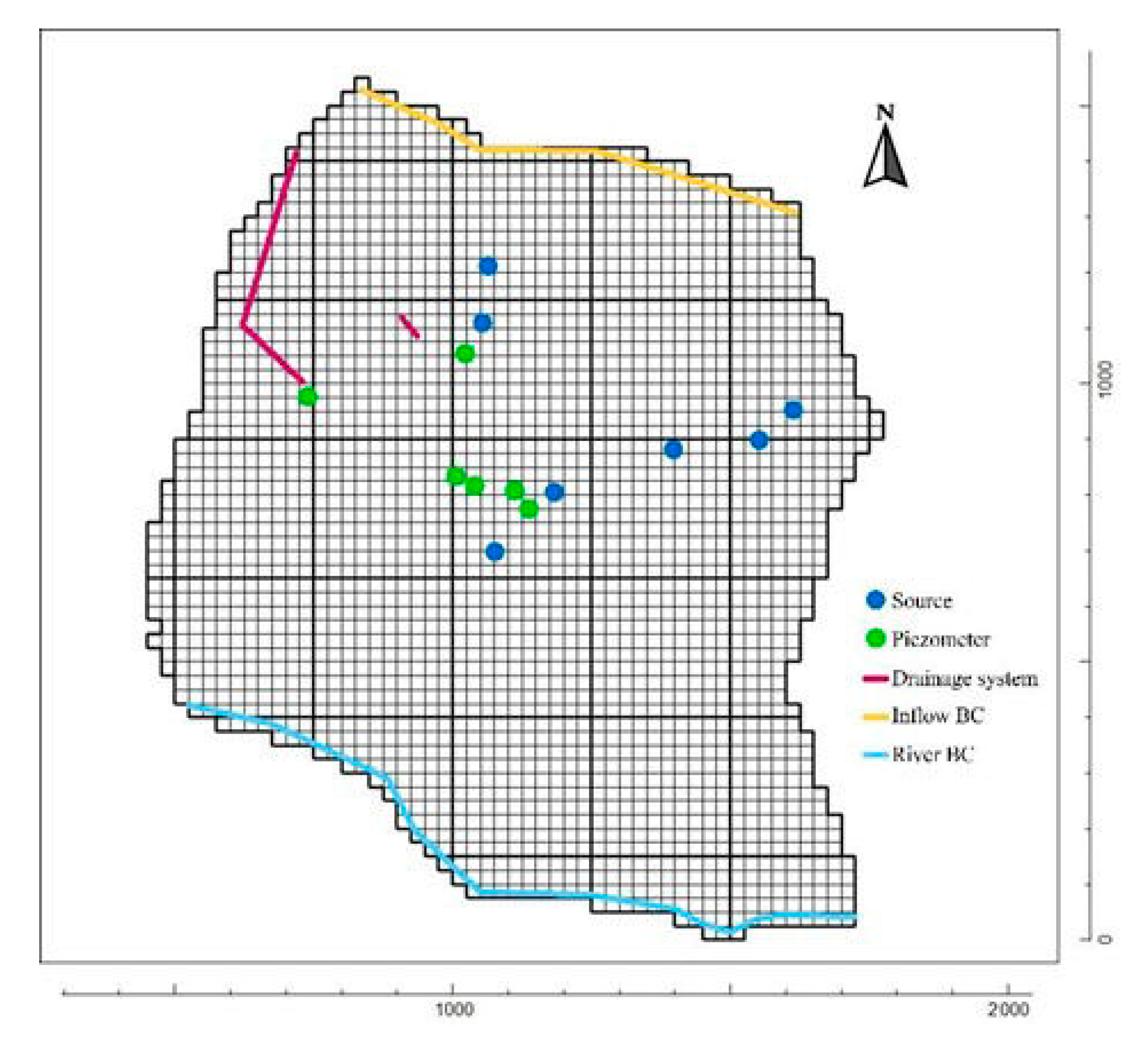
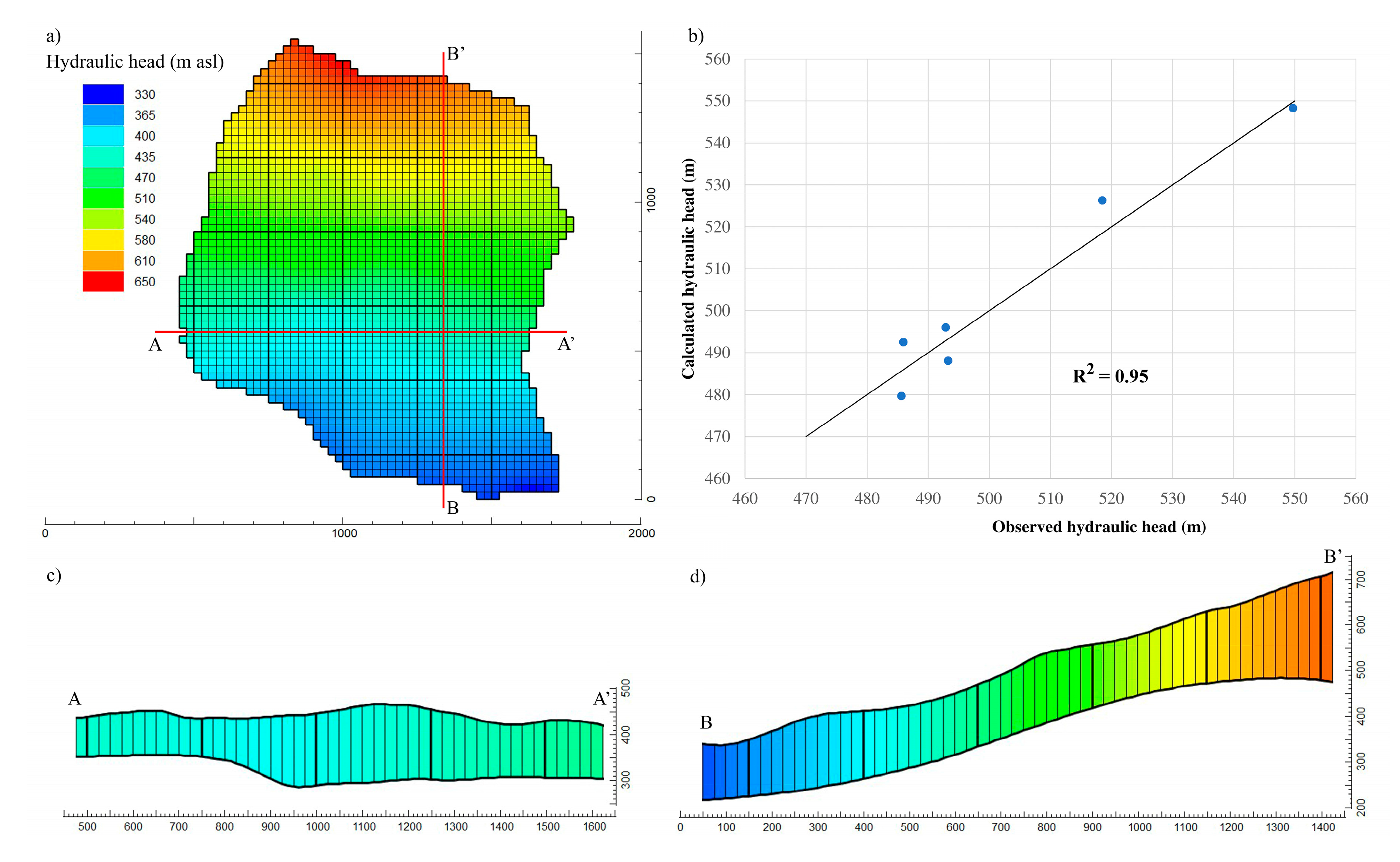
2.3.1. Hydrogeological Model

A three-dimensional heterogeneous model of the phreatic aquifer flowing into the study area, and working in steady state conditions, was developed. The model domain covers an area of about 1.5 km2 and is based on the morphological and geological reconstruction of the hillside affected by the landslide (Figure 3 and Figure 5). The 3-D geological model was compiled by integrating the surface geological map, with recently acquired and reconstructed vertical cross-sections (Section 2.1). These latter were used to recreate the layout of the aquifer bottom via an ordinary kriging approach. The ground level profile, instead, was realized using DEM data. The whole domain was horizontally discretized by a mesh of 25 × 25 m2 square elements. The vertical extent of the model is covered by a single layer, it has a variable thickness (in a range between 10 to 50 m) that follows the trend of the impermeable formation constituting the bottom of the superficial aquifer, and it is designed to replicate the heterogeneity created by the permeable geological formations across the area (Figure 7). The horizontal hydraulic conductivities of the geological formations (Figure 3 and Figure 5) are derived from Table 2. The vertical hydraulic conductivities were set to be a tenth of the horizontal ones, as has been done in many modeling applications, e.g., [68,69,70,71]. Faults, and their influence on groundwater flow, were been considered in the model, as their occurrence in the circumscribed model domain is minor, and furthermore, detailed information on their characteristics is not available.
No flow conditions were assigned to the east and west boundaries, while an inlet flow condition was set at the north boundary. The MODFLOW River Package was then used to simulate the surface water/groundwater interaction at the south boundary (Figure 8). The permanent water course, involved as a boundary condition in the modeling process, is the Corace river. Its monthly average flowrate ranges between a maximum of 9.71 m3/s, in the winter season, and a minimum of 0.446 m3/s during the summertime [72]. So, the variable flowrate will be proportional to the difference between the river stage and the hydraulic head in the aquifer, i.e., groundwater can leave the aquifer through the river boundary when the hydraulic head in the cell is higher than the river stage; otherwise, surface water can enter the aquifer through the river boundary when the head in the cell is below the river stage.
A natural aquifer recharge from rainfall N = 41 mm/y was homogeneously distributed on the model top according to the results of the water balance for the area under investigation.
The water balance can be described using the formula:
P i = E t i + R i + N i + Δ S i
where P i is the precipitation (L), E t i is the evapotranspiration (L), N i is the infiltration toward the aquifer (L), R i is the runoff (L), and Δ S i is the variation in the water storage of the soil (L). All the above-described quantities refer to the i-th month. The evapotranspiration E t i can be calculated with the method of Thornthwaite [73] based on the relationship existing between potential evapotranspiration and the average monthly temperature. The runoff R i was obtained using the infiltration curve method based on the Curve Number Method [74]. The water capacity of the ground, or field capacity, can be figuratively represented by a water-soaked sponge retaining its water content as long as the forces at play prevent its runoff. The water amount that does not runoff or evaporate seeps into the ground. If the ground is dry, the first part of this water is used to replenish the water reserve. This water asset will then be used by plants during the periods in which rain is not able to meet their water demand. The water reserve grows, until reaching the field capacity, during the rainy season while yielding the stored water when the net rain ( P i R i ) is less than evapotranspiration. When the water availability exceeds the potential evapotranspiration, and the water reserve reaches the maximum field capacity, the aquifer is recharged. Under these conditions, the variation in the water storage Δ S i is zero, and the value of the net vertical infiltration comes from the following relation:
N i = P i R i E t i
Drainage systems and springs, described in Section 2.2 and falling within the domain, were included into the model. Monitored wells and piezometers were also placed within the model and taken into consideration during the calibration procedure initially set-up to estimate the flowrate entering the system from the north inflow boundary condition (Figure 8).
As already said in the previous section, the automatic iterative optimization procedure was driven by UCODE-2005 [68]. The hydraulic head values, calculated at the model observation points and representing the monitoring wells and piezometers, were compared with the measured data. The procedure changed the values of the flowrate until the deviation between calculated and observed values reached a minimum value.

3. Results and Discussion

The first modeling stage, represented by the inversion of the hydraulic head data, was performed to quantify the possible inlet of a flowrate from the northern boundary. The outcomes of the model at the end of the iterative optimization procedure depict a situation in which the calculated hydraulic head distribution always overcomes the observed one by several meters. The sole contribution provided by the rain is sufficient to create conditions for which the entire domain is completely flooded. This unrealistic scenario can only be attributed to the adopted hydraulic conductivity values, which are too low to allow the model to manage even only those forcings of known entity (i.e., rain recharge).
For this reason, the optimization procedure, described in the previous section, was run again to evaluate both the flow rate entering the northern boundary and the value of an equivalent hydraulic conductivity for the aquifer capable of ensuring the compliance with the observed hydraulic heads and even an incoming flow rate at least comparable to that measured at the springs. In this second modeling phase, the aquifer was then turned into a homogeneous medium, without changing the geometrical layout, as the number of available observed data samples was not sufficient to guide and constrain the estimation of the parameters of the previous heterogeneous system. The estimated hydraulic conductivity of the equivalent homogeneous system resulted in a value of 2.7 × 10⁻⁶ m/s, which was two orders of magnitude higher than the previous permeabilities. This result, obtained for the homogeneous configuration, indirectly took also into account the effect of faults in the observed hydraulic head distribution adopted in the inversion process.
The reason of this difference between the slug tests’ estimation and the numerical model inversion can be ascribed to different observation scales of the two estimates, local for the first and regional for the second. Metamorphic aquifers, in fact, are characterized by a network of secondary connections of diverse orders and degrees that, among the main fractures, realizes a continuous variation in the hydrodynamic properties at different scales defining the modulus and direction of the groundwater flow. Moreover, the slug tests were all carried out in the landslide body resulting in close permeability values for all of them.
The estimated equivalent hydraulic conductivity value (2.7 × 10⁻⁶ m/s) enables a flow rate of 39.7 L/s entering the Northern boundary. This entry flow rate contemporarily fits the hydraulic heads of the monitored wells and piezometers and provides a groundwater flow even after the springs’ feed (Figure 9a). In fact, the estimated entering flow rate is of the same order of magnitude as that of the measured springs outlets (Section 2.3.1). The goodness of the fit is shown in the scatterplot having a determination coefficient R2 equal to 0.95 (Figure 9b).

4. Conclusions

In this work, an extensive campaign of field (hydro-geo-physical) measurements and a first modeling attempt of the Gimigliano aquifer are presented. The mathematical model was able to estimate the equivalent permeability of the Gimigliano aquifer and the presence of a lateral recharge from a deep confining aquifer. The adopted inverse approach provided a hydraulic conductivity of 2.7 × 10⁻⁶ m/s and a flow rate entering the northern boundary of 39.7 L/s.
The estimated hydraulic conductivity was almost one order of magnitude higher than the permeabilities estimated by means of slug tests. The reason for this discrepancy between the slug tests’ estimation and the numerical model inversion can be found in the different observation scales of the two estimates, very small for the first and regional for the latter. In fact, aquifers made up of metamorphic rocks include, among the main fractures, a network of secondary connections of different order and degree that determines, at different observation scales, a variation in the aquifer hydraulic properties defining the modulus and direction of the groundwater flow. Moreover, as a validation of our findings, the estimated lateral flow rate feeding the aquifer with a contribution of 39.7 L/s was of the same order of magnitude as the measured springs outlets.
So, as a conclusion, we argue that the hydraulic conductivity of metamorphic aquifers cannot be estimated only by field tests having a local investigation extent, but an inverse modeling approach is required, at a regional scale, which also takes into account the hydrological balance of the aquifer.

Author Contributions

All the authors contributed, in equal measures, to the implementation of the research, to the analysis of the results, and to the drafting the manuscript. All authors have read and agreed to the published version of the manuscript.

Funding

This research was funded by Regione Calabria: Convenzione per lo svolgimento di attività di consulenza tecnico-scientifica e di monitoraggio per i comuni di Gimigliano e Maierato (O.P.C.M. n.3862 del 31/03/2010).

Data Availability Statement

The data presented in this study are available on request from the corresponding author.

Conflicts of Interest

The authors declare no conflict of interest.

References

  1. Gustafson, G.; Krásny, J. Crystalline rock aquifers: Their occurrence, use and importance. Appl. Hydrogeol. 1994, 2, 64–75. [Google Scholar] [CrossRef]
  2. Wright, E.P.; Burgess, W.G. The Hydrogeology of Crystalline Basement Aquifers in Africa. Geol. Soc. Spec. Publ. 1992, 66, 264. [Google Scholar] [CrossRef]
  3. Baiocchi, A.; Dragoni, W.; Lotti, F.; Piacentini, S.M.; Piscopo, V. A Multi-Scale Approach in Hydraulic Characterization of a Metamorphic Aquifer: What Can Be Inferred about the Groundwater Abstraction Possibilities. Water 2015, 7, 4638–4656. [Google Scholar] [CrossRef] [Green Version]
  4. Stober, I.; Bucher, K. Hydrogeology of Crystalline Rocks; Kluwer Academic Publishers: Dordrecht, The Netherlands, 2003. [Google Scholar]
  5. Dewandel, B.; Lachassagne, P.; Wyns, R.; Maréchal, J.C.; Krishnamurthy, N.S. A generalized 3-D geological and hydrogeological conceptual model of granite aquifers controller by single or multiphase weathering. J. Hydrol. 2006, 320, 260–284. [Google Scholar] [CrossRef]
  6. Sharp, J.M. Fractured Rock Hydrogeology; Taylor & Francis: London, UK, 2014. [Google Scholar]
  7. Tsang, Y.W.; Tsang, C.F.; Hale, F.V.; Dverstorp, B. Tracer transport in a stochastic continuum model of fractured media. Water Resour. Res. 1996, 32, 3077–3092. [Google Scholar] [CrossRef]
  8. Hsieh, P.A. Scale effects in fluid flow through fractured geological media. In Scale Dependence and Scale Invariance in Hydrology; Sposito, G., Ed.; Cambridge Univ. Press: Cambridge, UK, 1998; pp. 35–353. [Google Scholar]
  9. Howard, K.W.K.; Hughes, M.; Charlesworth, D.L.; Ngobi, G. Hydrogeologic evaluation of fracture permeability in crystalline basement aquifers of Uganda. Hydrogeol. J. 1992, 1, 55–65. [Google Scholar] [CrossRef]
  10. Maréchal, J.C.; Dewandel, B.; Subrahmanyam, K. Use of hydraulic tests at different scales to characterize fracture network properties in the weathered-fractured layer of a hard rock aquifer. Water Resour. Res. 2004, 40, W11508. [Google Scholar] [CrossRef] [Green Version]
  11. de Marsily, G.; Lavedan, G.; Boucher, M.; Fasanino, G. Interpretation of interference tests in a well field using geostatistical techniques to fit the permeability distribution in a reservoir model. In Geostatistics for Natural Resources Characterization, Part 2; NATO Advanced Study Institute: Dordrecht, The Netherlands, 1984; pp. 831–849. [Google Scholar]
  12. Ahmed, S.; de Marsily, G. Comparison of geostatistical methods for estimating transmissivity using data on transmissivity and specific capacity. Water Resour. Res. 1987, 23, 1717–1737. [Google Scholar] [CrossRef]
  13. Nastev, M.; Savard, M.; Lapcevic, P.; Lefebvre, R.; Martel, R. Hydraulic properties and scale effects investigation in regional rock aquifers, southwestern, Quebec, Canada. Hydrogeol. J. 2004, 12, 257–269. [Google Scholar] [CrossRef]
  14. Patriarche, D.; Castro, M.C.; Goovaerts, P. Estimating regional hydraulic conductivity fields—A comparative study of geostatistical methods. Math. Geol. 2005, 37, 587–613. [Google Scholar] [CrossRef]
  15. Razack, M.; Lasm, T. Geostatistical estimation of the transmissivity in a highly fractured metamorphic and crystalline aquifer (Man-Danane Region, Western Ivory Coast). J. Hydrol. 2006, 325, 164–178. [Google Scholar] [CrossRef]
  16. Li, W.; Englert, A.; Cirpka, O.A.; Vanderborght, J.; Vereecken, H. Twodimensional characterization of hydraulic heterogeneity by multiple pumping tests. Water Resour. Res. 2007, 43, W04433. [Google Scholar] [CrossRef] [Green Version]
  17. Straface, S.; Yeh, T.C.J.; Zhu, J.; Troisi, S.; Lee, C.H. Sequential aquifer tests at a well field, Montalto Uffugo Scalo, Italy. Water Resour. Res. 2007, 43, W07432. [Google Scholar] [CrossRef]
  18. Kolterman, C.E.; Gorelick, S.M. Heterogeneity in sedimentary deposits: A review of structure-imitating, process-imitating, and descriptive approaches. Water Resour. Res. 1996, 32, 2617–2658. [Google Scholar] [CrossRef]
  19. de Marsily, G.; Delay, F.; Gonçalvès, J.; Renard, P.H.; Teles, V.; Violette, S. Dealing with spatial heterogeneity. Hydrogeol. J. 2005, 13, 161–183. [Google Scholar] [CrossRef]
  20. Straface, S.; Chidichimo, F.; Rizzo, E.; Riva, M.; Barrash, W.; Revil, A.; Cardiff, M.; Guadagnini, A. Joint inversion of steady-state hydrologic and self-potential data for 3D hydraulic conductivity distribution at the Boise Hydrogeophysical Research Site. J. Hydrol. 2011, 407, 115–128. [Google Scholar] [CrossRef]
  21. Neuman, S.P. Calibration of distributed parameter groundwater flow models viewed as a multiple-objective decision process under uncertainty. Water Resour. Res. 1973, 9, 1006–1021. [Google Scholar] [CrossRef]
  22. Yeh, W.W.G. Review of parameter estimation procedures in groundwater hydrology: The inverse problem. Water Resour. Res. 1986, 22, 95–108. [Google Scholar] [CrossRef]
  23. de Marsily, G.; Delhomme, J.P.; Delay, F.; Buoro, A. 40 years of inverse problems in hydrogeology. C. R. L’academie Sci. Ser. IIA—Earth Planet Sci. 1999, 329, 73–87. [Google Scholar] [CrossRef]
  24. Carrera, J.; Alcolea, A.; Medina, A.; Hidalgo, J.; Slooten, L.J. Inverse problem in hydrogeology. Hydrogeol. J. 2005, 13, 206–222. [Google Scholar] [CrossRef]
  25. Straface, S. Estimation of transmissivity and storage coefficient by means of a derivative method using the early-time drawdown. Hydrogeol. J. 2009, 17, 1679–1687. [Google Scholar] [CrossRef]
  26. Kelley, W.E. Geoelectrical sounding for estimating hydraulic conductivity. Groundwater 1977, 15, 420–425. [Google Scholar] [CrossRef]
  27. Urish, D.W. Electrical resistivity-hydraulic conductivity relationship in glacial outwash aquifers. Water Resour. Res. 1981, 17, 1401–1408. [Google Scholar] [CrossRef]
  28. Vouillamoz, J.M.; Descloitres, M.; Toe, G.; Legchenko, A. Characterization of crystalline basement aquifers with MRS: Comparison with boreholes and pumping tests data in Burkina Faso. Near Surf. Geophys. 2005, 3, 205–213. [Google Scholar] [CrossRef]
  29. Straface, S.; Rizzo, E.; Chidichimo, F. Estimation of hydraulic conductivity and water table map in a large scale laboratory model by means of the self-potential method. J. Geophys. Res. 2010, 115, B06105. [Google Scholar] [CrossRef]
  30. Chidichimo, F.; De Biase, M.; Rizzo, E.; Masi, S.; Straface, S. Hydrodynamic parameters estimation from self-potential data in a controlled full scale site. J. Hydrol. 2015, 522, 572–581. [Google Scholar] [CrossRef]
  31. Ahmed, S.; de Marsily, G.; Talbot, A. Combined use of hydraulic and electrical properties of an aquifer in a geostatistical estimation of transmissivity. Groundwater 1988, 26, 78–86. [Google Scholar] [CrossRef]
  32. Fallico, C.; Vita, M.C.; De Bartolo, S.; Straface, S. Scaling Effect of the Hydraulic Conductivity in a Confined Aquifer. Soil Sci. 2012, 177, 385–391. [Google Scholar] [CrossRef]
  33. Dewandel, B.; Maréchal, J.C.; Bour, O.; Ladouche, B.; Ahmed, S.; Chandra, S.; Pauwels, H. Upscaling and regionalizing hydraulic conductivity and effective porosity at watershed scale in deeply weathered crystalline aquifers. J. Hydrol. 2012, 416–417, 83–97. [Google Scholar] [CrossRef]
  34. Paillet, F.L. Flow modeling and permeability estimation using borehole flow logs in heterogeneous fractured formations. Water Resour. Res. 1998, 34, 997–1010. [Google Scholar] [CrossRef]
  35. Maréchal, J.C.; Dewandel, B.; Ahmed, S.; Galeazzi, L.; Zaidi, F.K. Combined estimation of specific yield and natural recharge in a semi-arid groundwater basin with irrigated agriculture. J. Hydrol. 2006, 329, 281–293. [Google Scholar] [CrossRef] [Green Version]
  36. Le Borgne, T.; Bour, O.; de Dreuzy, J.; Davy, P.; Touchard, F. Equivalent mean flow models for fractured aquifers: Insights from a pumping test scaling interpretation. Water Resour. Res. 2004, 40, W03512. [Google Scholar] [CrossRef]
  37. Le Borgne, T.; Bour, O.; Paillet, F.L.; Caudal, J.P. Assessment of preferential flow path connectivity, and hydraulic properties at single-borehole and crossborehole scales in a fractured aquifer. J. Hydrol. 2006, 328, 347–359. [Google Scholar] [CrossRef]
  38. Courtois, N.; Lachassagne, P.; Wyns, R.; Blanchin, R.; Bougaïré, F.D.; Somé, S.; Tapsoba, A. Large-Scale Mapping of Hard-Rock Aquifer Properties Applied to Burkina Faso. Groundwater 2010, 48, 269–283. [Google Scholar] [CrossRef]
  39. Guihéneuf, N.; Boisson, N.; Bour, O.; Dewandel, B.; Perrin, J.; Dausse, A.; Viossanges, M.; Chandra, S.; Ahmed, S.; Maréchal, J.C. Groundwater flows in weathered crystalline rocks: Impact of piezometric variations and depth-dependent fracture connectivity. J. Hydrol. 2014, 511, 320–334. [Google Scholar] [CrossRef]
  40. Lee, C.H.; Chang, J.L.; Deng, B.W. A continuum approach for estimating permeability in naturally fractured rocks. Eng. Geol. 1995, 39, 71–85. [Google Scholar] [CrossRef]
  41. Scanlon, B.R.; Mace, R.E.; Barrett, M.E.; Smith, B. Can we simulate regional groundwater flow in a karst system using equivalent porous media models? Case study, Barton Springs Edwards aquifer, USA. J. Hydrol. 2003, 276, 135–158. [Google Scholar] [CrossRef]
  42. Lemieux, J.M.; Therrien, R.; Kirkwood, D. Small scale study of groundwater flow in a fractured carbonate-rock aquifer at the St-Eustache quarry, Québec, Canada. Hydrogeol. J. 2006, 14, 603–612. [Google Scholar] [CrossRef]
  43. Long, J.C.S.; Remer, J.S.; Wilson, C.R.; Witherspoon, P.A. Porous media equivalents for networks of discontinuous fractures. Water Resour. Res. 1982, 18, 645–658. [Google Scholar] [CrossRef] [Green Version]
  44. Hsieh, P.A.; Neuman, S.P.; Stiles, G.K.; Simpson, E.S. Field determination of the three-dimensional hydraulic conductivity tensor of anisotropic media: 2 Methodology and application to fractured rocks. Water Resour. Res. 1985, 21, 1667–1676. [Google Scholar] [CrossRef]
  45. Neuman, S.P. Stochastic Continuum Representation of Fractured Rock Permeability as an Alternative to the Rev and Fracture Network Concepts. In Proceedings of the 28th US Symposium on Rock Mechanics, Tucson, AZ, USA, 29 June–1 July 1987. [Google Scholar]
  46. Neuman, S.P. Trends, prospects and challenge in quantifying flow and transport through fractured aquifer. Hydrogeol. J. 2005, 13, 124–147. [Google Scholar] [CrossRef]
  47. Bradbury, K.R.; Muldoon, M.A.; Zaporec, A.; Levy, J. Delineation of Wellhead Protection Areas in Fractured Rocks; US EPA Technical Guidance Document, EPA 570/9-91-009; EPA: Washington, DC, USA, 1991. [Google Scholar]
  48. Baiocchi, A.; Dragoni, W.; Lotti, F.; Piscopo, V. Sustainable yield of fractured rock aquifers: The case of crystalline rocks of Serre Massif (Calabria, Southern Italy). In Fractured Rock Hydrogeology; Sharp, J.M., Ed.; Taylor &Francis Group: London, UK, 2014; pp. 79–97. [Google Scholar]
  49. Domenico, P.A.; Schwartz, F.W. Physical and Chemical Hydrogeology; John Wiley & Sons: New York, NY, USA, 1990; 824p. [Google Scholar]
  50. Heath, R.C. Basic Groundwater Hydrology; U.S. Geological Survey Water-Supply Paper 2220: Washington, DC, USA, 1983; 86p. [Google Scholar]
  51. Dragoni, W. Some considerations on climatic changes, water resources and water needs in the Italian region south of the 43° N. In Water, Environment and Society in Times of Climatic Change; Issar, A., Brown, N., Eds.; Kluwer Academic Publishers: Dordrecht, The Netherlands, 1998; pp. 241–271. [Google Scholar]
  52. Bianchini, S.; Cigna, F.; Del Ventisette, C.; Moretti, S.; Casagli, N. Monitoring Landslide-Induced Displacements with TerraSAR-X Persistent Scatterer Interferometry (PSI): Gimigliano Case Study in Calabria Region (Italy). Int. J. Geosci. 2013, 4, 1467–1482. [Google Scholar] [CrossRef] [Green Version]
  53. Van Dijk, J.P.; Bello, M.; Brancaleoni, G.P.; Cantarella, G.; Costa, V.; Frixa, A.; Golfetto, F.; Merlini, S.; Riva, M.; Torricelli, S.; et al. A regional structural model for the northern sector of the Calabrian Arc (southern Italy). Tectonophysics 2000, 324, 267–320. [Google Scholar] [CrossRef]
  54. Tansi, C.; Muto, F.; Critelli, S.; Iovine, G. Neogene-Quaternary strike-slip tectonics in the central Calabrian Arc (Southern Italy). J. Geodyn. 2007, 43, 393–414. [Google Scholar] [CrossRef]
  55. Brutto, F.; Muto, F.; Loreto, M.F.; De Paola, N.; Tripodi, V.; Critelli, S.; Facchin, L. The Neogene-Quaternary geodynamic evolution of the central Calabrian Arc: A case study from the western Catanzaro Trough basin. J. Geodyn. 2016, 102, 95–114. [Google Scholar] [CrossRef] [Green Version]
  56. Bonardi, G.; Cello, G.; Perrone, V.; Tortorici, L.; Turco, E.; Zupetta, A. Palinspastic restoration of the northern sector of the Calabro-Peloritani arc in a semiquantitative model. Boll. Soc. Geol. Ital. 1982, 101, 259–274. [Google Scholar]
  57. Tortorici, L. Lineamenti geologico-strutturali dell’Arco Calabro Peloritano (Geologic structural lineaments of the Calabrian-Peloritan Arc). Soc. Ital. Mineral. Petrogr. 1982, 38, 927940. [Google Scholar]
  58. Critelli, S.; Muto, F.; Perri, F.; Tripodi, V. Interpreting provenance relations from sandstone detrital modes, southern Italy foreland region: Stratigraphic record of the Miocene tectonic evolution. Mar. Petrol. Geol. 2017, 87, 47–59. [Google Scholar] [CrossRef]
  59. Amodio-Morelli, L.; Bonardi, G.; Colonna, V.; Dietrich, D.; Giunta, G.; Ippolito, F.; Liguori, V.; Lorenzoni, S.; Paglionico, A.; Perrone, V.; et al. L’arco Calabro-Peloritano nell’orogene appenninico Maghrebide. Mem. Soc. Geol. Ital. 1976, 17, 1–60. [Google Scholar]
  60. Bouwer, H.; Rice, R.C. A slug test for determining hydraulic conductivity of unconfined aquifers with completely or partially penetrating wells. Water Resour. Res. 1976, 12, 423. [Google Scholar] [CrossRef] [Green Version]
  61. Zlotnik, V. Interpretation of slug and packer tests in anisotropic aquifers. Groundwater 1994, 32, 761. [Google Scholar] [CrossRef]
  62. Butler, J.J. The Design, Performance, and Analysis of Slug Tests; Lewis Publisher CRC Press: Lawrence, KS, USA, 1998; ISBN 1566702305. [Google Scholar]
  63. Pezzotta, G.; Burton, A.N.; Hughes, D.O. Carta Geologica della Calabria: Nota Illustrativa delle Tavolette Appartenenti al Foglio 242 della Carta Topografica D’italia; Cassa del Mezzogiorno: Roma, Italy, 1973. [Google Scholar]
  64. Repertorio Nazionale dei Dati Territoriali (RNDT). Available online: https://geodati.gov.it/geoportale/geoviewer/ (accessed on 14 September 2022).
  65. Bear, J. Hydraulics of Groundwater; McGraw-Hill Publishing: New York, NY, USA, 1979. [Google Scholar]
  66. Harbaugh, A.W. MODFLOW-2005: The U.S. Geological Survey modular ground-water model—The ground-water flow process. In Book 6: Modeling Techniques, Section A. Ground-Water; US Geological Survey: Reston, VI, USA, 2005; p. 6-A16. [Google Scholar]
  67. Poeter, E.P.; Hill, M.C.; Banta, E.R.; Steffen, M.; Steen, C. UCODE-2005 and six other computer codes for universal sensitivity analysis, calibration, and uncertainty evaluation constructed using the JUPITER API. In U.S. Geological Survey Techniques and Methods; US Geological Survey: Reston, VI, USA, 2008; p. 6-A11. [Google Scholar]
  68. De Biase, M.; Chidichimo, F.; Maiolo, M.; Micallef, A. The Impact of Predicted Climate Change on Groundwater Resources in a Mediterranean Archipelago: A Modelling Study of the Maltese Islands. Water 2021, 13, 3046. [Google Scholar] [CrossRef]
  69. De Biase, M.; Chidichimo, F.; Micallef, A.; Cohen, D.; Gable, C.; Zwinger, T. Past and future evolution of the onshore-offshore groundwater system of a carbonate archipelago: The case of the Maltese Islands, central Mediterranean Sea. Front. Water 2023, 4, 1068971. [Google Scholar] [CrossRef]
  70. Haroon, A.; Micallef, A.; Jegen, M.; Schwalenberg, K.; Karstens, J.; Berndt, C.; Garcia, X.; Kühn, M.; Rizzo, E.; Fusi, N.C.; et al. Electrical resistivity anomalies offshore a carbonate coastline: Evidence for freshened groundwater? Geophys. Res. Lett. 2021, 48, e2020GL091909. [Google Scholar] [CrossRef]
  71. Lemieux, J.M.; Hassaoui, J.; Molson, J.; Therrien, R.; Therrien, P.; Chouteau, M.; Ouellet, M. Simulating the impact of climate change on the groundwater resources of the Magdalen Islands, Québec, Canada. J. Hydrol. Reg. Stud. 2015, 3, 400–423. [Google Scholar] [CrossRef] [Green Version]
  72. ARPACAL—Centro Funzionale Multirischi. Available online: https://www.cfd.calabria.it/index.php (accessed on 27 February 2023).
  73. Thornthwaite, C.W. An Approach toward a Rational Classification of Climate. Geogr. Rev. 1948, 38, 55–94. [Google Scholar] [CrossRef]
  74. Cronshey, R.; McCuen, R.H.; Miller, N.; Rawls, W.; Robbins, S.; Woodward, D.; Chenoweth, J.; Hamilton, S.; Merkel, W.; Rallison, R.; et al. Urban Hydrology for Small Watersheds—Technical Release 55, 2nd ed.; United States Department of Agriculture (USDA): Washington, DC, USA, 1986; p. 164. [Google Scholar]
Figure 1. Hydraulic conductivity of selected consolidated and unconsolidated geologic materials (from [49,50]).
Hydrology 10 00080 g001
Figure 2. Schematic geological map of the northern Calabria. The black square in the southeastern sector indicates the location of the study area. Modified after Dijk et al. ii 2000 [53] and Tansi et al. ii 2007 [54].
Hydrology 10 00080 g002
Figure 3. Detailed geological map of the Corace River-Gimigliano village area. A-A’ is the geological cross-section trace. In the central sector (white color), the landslide and slope deposits are mapped.
Hydrology 10 00080 g003
Figure 4. Model of resistivity of the B-B’ (ERT) longitudinal section.
Hydrology 10 00080 g004
Figure 5. Geological cross-section along the longitudinal A-A’ trace (Figure 3). The 2D geological-structural model is the result of the field survey, borehole stratigraphies, and ERT interpretation.
Hydrology 10 00080 g005
Figure 6. Logarithm of hydraulic head displacement (H) and measurement error bars vs. time plot of slug tests performed in boreholes S2a (a), S2b (b), S2c (c), S3b (d), and S3c (e) at the Gimigliano study area.
Hydrology 10 00080 g006aHydrology 10 00080 g006b
Figure 7. (a) Surface geological formations included into the model domain depicting zones with different hydrodynamic parameters; (b) 3D view of the model; (c) cross-section A-A’ and (d) cross-section B-B’ depicting the thickness layout of the model.
Hydrology 10 00080 g007
Figure 8. Boundary conditions together with relevant elements included in the model.
Hydrology 10 00080 g008
Figure 9. (a) Hydraulic head distribution at the end of the optimization procedure; (b) scattergraph of the observed and calculated hydraulic head values; (c) hydraulic distribution in cross sections A-A’ and (d) B-B’ also displayed in Figure 7.
Hydrology 10 00080 g009
Table 1. Geometrical characteristics of the boreholes drilled into the aquifer and water table depths measured during the spring season.
BoreholeDiameter (mm)Borehole Depth (m)Filter Depth (m)Water Table Depth (m)
S1a2208.003.00–8.00Dry
S1b16038.0033.00–38.00Dry
S1c16051.0043.00–50.00Dry
S2a16013.006.00–13.008.75
S2b16025.0016.00–25.008.75
S2c16042.0030.00–42.008.75
S3a1608.002.00–8.00Dry
S3b16030.0014.00–30.0020.30
S3c16048.0038.00–47.0033.60
SITa16040.0015.00–25.0011.95
SITb16040.000.00–10.00Dry
SITc10840.000.00–40.0010.05
SP16060.000.00–60.0032.73
Table 2. Summary of the Slug Tests’ results carried out in different piezometers. The table shows the lithology and the hydraulic conductivity obtained with the Bouwer–Rice method.
BoreholeLithologyHydraulic Conductivity (m/s)
S1aHighly weathered metabasitesna (dry)
S1bHighly fractured schistsna (dry)
S1cWeathered and locally intact metabasitesna (dry)
S2aHighly weathered phyllites9.90 × 10−8
S2bHighly weathered metabasites6.77 × 10−8
S2cHighly weathered serpentinites7.51 × 10−8
S3aHighly weathered metabasitesna (dry)
S3bMetabasites with quartz vein1.80 × 10−7
S3cWeathered metabasites reduced to coarse sands7.44 × 10−8
Table 3. Springs/Sources (S) detected in the study area. The reported values were observed in February 2011.
NameTypeFlowrate (L/s)
CalvarioS1.0
SS Maria di PortoS0.1
San Giorgio 1S1.0
San Giorgio 2S2.0
AgoniaS1.0
IannuliS2.0
LoccoS3.5
Disclaimer/Publisher’s Note: The statements, opinions and data contained in all publications are solely those of the individual author(s) and contributor(s) and not of MDPI and/or the editor(s). MDPI and/or the editor(s) disclaim responsibility for any injury to people or property resulting from any ideas, methods, instructions or products referred to in the content.

