Article

Modeling Surface Water–Groundwater Interactions: Evidence from Borkena Catchment, Awash River Basin, Ethiopia

by
Wallelegn Jene Gobezie
1,
Ermias Teferi
2,3,
Yihun T. Dile
4,
Haimanote K. Bayabil
5,
Gebiaw T. Ayele
6,* and
Girma Y. Ebrahim
7
1
Ethiopian Institute of Water Resources, Addis Ababa University, Addis Ababa P.O. Box 1176, Ethiopia
2
Center for Environment and Development Studies, Addis Ababa University, Addis Ababa P.O. Box 1176, Ethiopia
3
Water and Land Resource Center (WLRC), Addis Ababa University, Addis Ababa P.O. Box 3880, Ethiopia
4
Spatial Sciences Laboratory in the Development of Ecosystem Sciences and Management, Texas A&M University, College Station, TX 77843, USA
5
Agricultural and Biological Engineering, Tropical Research and Education Centre, Institute of Food and Agricultural Sciences, University of Florida, Homestead, FL 33031, USA
6
Australia River Institute and School of Engineering, Griffith University, Nathan, QLD 4111, Australia
7
International Water Management Institute, Addis Ababa P.O. Box 5689, Ethiopia
*
Author to whom correspondence should be addressed.
Hydrology 2023, 10(2), 42; https://doi.org/10.3390/hydrology10020042
Submission received: 19 November 2022 / Revised: 22 January 2023 / Accepted: 29 January 2023 / Published: 3 February 2023

Abstract

:
The availability of sufficient water resources is critical for sustainable social and economic development globally. However, recurrent drought has been a precursor to inadequate water supply in the case of Borkena Catchment, Awash River Basin, Ethiopia. To support the conjunctive use and management of surface water and groundwater in Borkena Catchment, an integrated model was developed using the SWAT–MODFLOW model. The model was designed to operate on a monthly time scale. The change in the water balance obtained from the SWAT–MODFLOW model provides a quantitative means to assess the effect of the climate variability and changes, as well as the impact of human activities, on water resources. To advance the understanding at the regional and local scales, surface water–groundwater interactions in the Borkena Catchment geochemical information and piezometer maps were integrated. The results show that the groundwater recharge in the study area is approximately 122 mm/a. The surface water–groundwater interaction results show that the areas around Harbu and Dessie are characterized as losing rivers, while the areas around Kemisse-Chefa and the highlands of Kutaber, where the Borkena River originates, are characterized as gaining rivers. A geochemical analysis indicated that there is an inter-basin groundwater transfer from the Abbay to the Awash basin. The integrated model generated key temporal and spatial information that is useful for the sustainable conjunctive management of surface and groundwater in Borkena Catchment for climate resilience in the face of climate variability and increasing demand.

1. Introduction

Groundwater and surface water are in continuous hydraulic interactions [1,2]. This interaction has practical consequences in the quantity and quality of water in either system [3]. The depletion and/or contamination of one of the systems will eventually affect the other.
Therefore, understanding groundwater and surface water interactions, hydrological processes, and hydrogeological systems of catchments and their vulnerability to natural stressors are very essential for proper water resource utilization and management [4]. Particularly, the interaction between groundwater and surface water is crucial in hydrological systems that rely on limited freshwater resources, such as the Borkena River Catchment [5]. Recently, the integrated management of groundwater (GW) and surface water (SW) resources is growing to meet the social and ecological flow requirements of both water resources. Such integrated GW and SW management requires information concerning the effects of groundwater on surface water systems and vice versa [6]. GW and SW interactions are often studied using models, which help to establish locations, characterize aquifer boundaries, and assess the amount of water within the systems, including recharge to the groundwater aquifer and flow to surface water [7]. These models are used to calculate the rate and direction of the movement of groundwater through aquifers and confining units in the subsurface, the exchange of surface and groundwater between aquifers, sources, and sinks, including other groundwater infusion and removal from an aquifer.
Modeling approaches that account for surface and groundwater modeling as one complex system are often known as integrated models. Integrated models are useful for solving complex water resources problems and contribute substantially to our understanding of the hydrology of watersheds, rivers, and aquifers. However, GW and SW modeling is not without a challenge. One of the challenges, for example, is the significant time scale differences between GW and SW processes [8]. Groundwater flow is in the order of magnitude slower than SW flow, as the groundwater response to natural and artificial drivers, such as climate variability, land use change, and groundwater extraction, can be damped [9,10,11,12]. Hence, such dynamics should be well captured in the GW and SW interactions modeling.
Few studies have assessed GW and SW interactions in catchments in Ethiopia [13,14,15]. The groundwater abstraction is considerably increasing without consistent quantification of surface water components and the extent available for extraction [16]. Therefore, the main objective of this study was to develop an integrated model to support conjunctive use and management of the surface and groundwater Borkena Catchment. The primary focus is to improve the understanding of the GW–SW interactions and their dynamics, as well as to provide the scientific information needed for water resources management.

2. Materials and Methods

2.1. Study Area

This study was conducted in the Borkena Catchment, which is located in the Awash River Basin in Ethiopia (Figure 1). The catchment covers a total area of ~1606 km2. It is geographically bounded between 39.3° and 39.7° longitude and 10.2° and 11.3° latitude.
The hydrogeological map of the study area is shown in Figure 2. The western volcanic escarpments and the eastern ridge that bound the alluvial valley aquifers are highly dissected by stream networks, often with the rugged topography of the study area. The valley plain alluvial aquifers often gently roll to the south with isolated hills as observed in the southern extreme part of the area. The elevation reaches 3500 m above sea level (m.a.s.l.) on the escarpment, whereas the wide Borkena graben lies at an average elevation of 1400 m.a.s.l.
A large area of the Borkena Catchment is under cultivation, dominantly covered by agricultural land (49.6%). Brush land and range land cover 20% and 15% of the watershed, respectively. The remaining part of the watershed is covered by barren land, wetlands, plantations, and forests (Table 1). The major soil types in the Borkena Catchment are lithic Leptosols and Eutric Vertisols (Table 2). The soil and land use/land cover maps of the study area were collected from the Ethiopian Ministry of Water and Energy (MoWE).

2.2. SWAT–MODFLOW Model Setup

2.2.1. SWAT Model Setup and Input Data

The SWAT model requires spatial and temporal data to simulate various hydrological processes. The required spatial data include the digital elevation model (DEM), land use, and soil. The DEM data had a resolution of 30 m, and it was used to discretize watershed characteristics. The DEM data were obtained from the Shuttle Radar Topographic Mission (SRTM) (https://earthexplorer.usgs.gov) (accessed on 15 September 2021). The land use and soil data were necessary to define the hydrological response units (HRUs), which are the smallest units in the SWAT model. The watershed delineation resulted in 12 sub-basins and 187 hydrological response units (HRUs). The multiple HRU option was selected to represent the different land use, soil, and slope classes in the catchment.
The daily rainfall, maximum/minimum temperatures, solar radiation, relative humidity, and wind speed data for the period 1979–2017 were obtained from the Ethiopian National Meteorological Services Agency (NMSA) for Combolcha and Kemisse stations. The stream flow data used for the SWAT model calibration and validation were obtained from the Ministry of Water and Energy (MoWE). The potential evapotranspiration was estimated using the Penman–Monteith method.

2.2.2. SWAT Model Calibration and Validation

The SWAT model was calibrated and validated using monthly observed stream flow for the period 2000–2007 and 2008–2014, respectively. The observed stream flow data for the period 1979–1981 were used for the model warm-up, which is important for balancing the different stocks in the catchment [17,18,19]. Initially, the parameters were manually calibrated, and thereafter automatic calibration with the SWAT–CUP was employed. The automatic calibration was conducted using the sequential uncertainty fitting (SUFI-2) algorithm. The SUFI-2 algorithm provides satisfactory model [20] performance while converging in a relatively smaller number of iterations. The SWAT model calibration and validation performances were assessed using three statistical parameters. These are coefficient of determination (R2), Nash–Sutcliff efficiency (NSE), and percent bias. The NSE is a normalized statistic that determines the relative magnitude of the residual variance compared to the observed data variance [21]. According to [22], the NSE can range from −∞ to 1. The PBIAS compares the volumetric difference between simulated and observed data. This study considered a simulation with a calibrated model satisfactory when an R2 > 0.6, NSE > 0.5, and PBIAS < ±15%.
The model performance before the model calibration was poor, with a coefficient of determination (R2) of 0.33, Nash–Sutcliffe efficiency (NSE) of 0.33, and PBIAS of −3.9%. This necessitated the need for model calibration, which provided a coefficient of determination (R2) of 0.68, Nash–Sutcliffe efficiency (NSE) of 0.66, and PBIAS of −2.7%. The validation of the model using independent monthly observed stream flow data for the period 2008–2014 showed an acceptable performance with an R2, NSE, and PBIAS of 0.64, 0.61, and 2.48%, respectively (Table 3). According to model evaluation guidelines [22], the model calibration provided an acceptable performance. The fitted values of the parameters for the calibration are presented in Table 4. The hydrograph results of the calibrated and validation periods of the observed and simulated flow in monthly estimation indicates similar trends in different seasons with acceptable ranges (Figure 3).

2.2.3. MODFLOW Model Setup

Conceptual Model

A hydrogeological map and cross-section were prepared to conceptualize the Borkena Catchment alluvial aquifer and tertiary volcanic aquifers. The groundwater flow in the alluvial aquifer is governed by the configuration of low to moderate permeable tertiary volcanic rocks that surround the alluvial formation from all directions, the high hydraulic conductivity of the aquifer material, the areal extent and thickness of the aquifer, and the groundwater recharge and groundwater discharge. Such information was used to construct the conceptual model (developed cross-sections and groundwater flow map) that describes the internal and external boundaries of the groundwater flow system, the inflow and outflow of water at these boundaries, and the overall effect of these boundaries on the groundwater flow in the aquifer. The Borkena Catchment alluvial aquifer is a natural subsurface reservoir filled by the runoff infiltration of large numbers of rivers mainly at the western and northern periphery of the alluvial aquifer and dammed by the low to moderate permeable tertiary volcanic formation in all directions.
Such a geological formation causes distributed discharge along the central and lower parts of the Borkena River through the confining thin (10 m) layer of clay [23]. Based on the KCVTW-02-19 and KCVTW-03-19 well completion reports [23,24,25,26], three boreholes were drilled 500, 600, and 512 m deep, and the alluvial aquifer thickness was found from 230 to 250 m. As of the data from the KCVTW-01-19 and KCVTW-02-19 well completion reports, the hydraulic conductivities of the volcanic aquifers in the two boreholes were calculated and were nearly similar and large enough to transfer water from one region to another region [23,24,25,26]. These unpublished report data were used for this study to process the existing borehole data for the calculation of the aquifer properties and the physicochemical analysis using aquifer test and aquacheme software, analyzed and discussed in the Section 3. The borehole data were collected from the Ethiopian Construction Design and Supervision Works Corporation, Water and Energy Design and Supervision Works Sector [23,24,25,26], and via field monitoring. Moreover, this study measured the additional water level of the boreholes using a deep meter to develop the hydrogeological, cross-section, and groundwater contour and flow maps.
The hydrogeological cross-section maps were developed to show the regional and local groundwater flows in the system and from out of the system. The borehole data observations indicated that the aquifers, especially at the middle, center, and southern center (along the Borkena River), appeared to be artesian (overflowing), providing a distributed groundwater discharge to the river. Some of the evidence that supports the aquifers in the Borkena Catchment being artesian and the groundwater contributing to the river flow include:
  • The base flow of the Borkena River increases after passing through the alluvial aquifers as it flows through the volcanic rock channel.
  • The boreholes drilled along the lowest elevation areas were artesian.
  • A large swamp developed at the southern part of the Borkena Catchment

Model Discretization

The model domain was divided into 47 rows and 23 columns, with a uniform grid size of 2000 × 2000 m. This resulted in 1081 grid cells. In designing the grid, the length-to-width ratio (aspect ratio) of the cells was kept close to one as much as possible to avoid numerical instabilities or errors. The model was discretized vertically into one layer. Since MODFLOW needs the ground surface elevation for the grid cell, the DEM that was used to set-up the SWAT model was used to define the top layer of the aquifer. The aquifer thickness of the Borkena Catchment was determined from the pumping test result of the existing boreholes’ static water level and the elevation difference with the borehole depth. The aquifer thickness, which includes both the alluvial and tertiary volcanic aquifers, was estimated to be ~280 m.

Aquifer Hydraulic Properties

The magnitude and spatial distribution of the aquifer properties, such as hydraulic conductivity and storage coefficient (specific storage and specific yield), are required for the MODFLOW model. Hydraulic conductivity is one of the highly variable parameters in space. Most of the studied drilled wells are located in the central part of the alluvial aquifers. Boreholes from 80 to 600 m in depth were found drilled mainly in Kutaber, Dessie, Combolcha, Harbu, Kemisse, and Chefa towns, and some of the boreholes fully penetrated the alluvial aquifer, which has a depth of 248 m, while the rest did not.
Hydraulic conductivity, which indicates the flow of water in an aquifer system, is one of the inputs to the MODFLOW model. The hydraulic conductivity of the area is highly variable due to the presence of different geologic structures. Pumping test data showed that acidic rocks, such as those in the Dessie area, have a hydraulic conductivity of 0.01 m/day, which increases to 36.6 m/day in the tertiary fractured volcanic aquifers and in the alluvial areas of Kombolcha, Kemisse, and Chefa. This study used an average hydraulic conductivity value of 3.38 m/day for the model. From the existing boreholes data, the transmissivity of the Borkena aquifer systems was calculated and ranged between 4.3 and 1895.6 m2/day. An average transmissivity value of 255.36 m2/day was used as input to the MODFLOW model.
The vertical-to-horizontal hydraulic conductivity anisotropy ratio is given by Kx/Kz in which Kz is the vertical hydraulic conductivity and Kx is the radial (horizontal) hydraulic conductivity [27]. The authors also reported that the values of Kx/Kz range between 0.1 and 10 for alluvial and volcanic aquifers, possibly as low as 0.01 when clay layers are present and from 0.01 to 1.5 for volcanic material, even if it is determined by the strata and fracture conditions of the geologic material. Therefore, this study used a Kx/Kz of 0.1 as input for MODFLOW.
The porosity of alluvial aquifers is reported in the range of 40–70% for clays, 35–50% for silts, 25–50% for sands, and 25–40% for gravels [27]. The porosity of fractured basalt rock is reported as 5–50% [28]. Since the alluvial aquifer in the Borkena Catchment is dominantly sand and gravel, a saturated average porosity of 30% or 0.3 was used in the MODFLOW model.
The specific yield determines the ratio of the volume of water that drains an aquifer because of gravity to the total volume of the saturated aquifer AA [29]. The specific yield of alluvial aquifers varies from 0.15 to 0.2. The alluvial aquifer for the Borkena Catchment was estimated to be ~0.15.
The specific storage of a saturated aquifer is the volume of water that a unit volume of aquifer releases from storage under a unit decline in hydraulic head. The specific storage of unconsolidated aquifers ranges from 0.00005 to 0.00168 [28,29]. This study used an average specific storage of 0.00015 for the MODFLOW model.

River–Aquifer Interactions

The flow between a river and an aquifer depends on the difference between the water level in the river and the groundwater head. The River Package of MODFLOW simulates stream–aquifer interactions based on three parameters: (i) river stage, (ii) river bed elevation, and (iii) conductance of the riverbed material. The river stages were determined using the median river elevation within the cell based on the observed river elevation and DEM data. The streambed conductance (Criv) controls the rate of water movement to or from a stream in response to the head gradient. Direct measurements of streambed conductance were not available, and it was fine-tuned during model calibration. Approximately 49 river cells were assigned using the river package after calculating the river conductance using Equation (1) (Table S2). The determination of the vertical hydraulic conductivity (Kv) of the entire riverbed has significant importance for the study of groundwater recharge [30]. Depending on the riverbed material, the hydraulic conductivity of the riverbed varies from 1 to 3 m/day. Therefore, an hydraulic conductivity of 1 m/d was used to represent the hydraulic conductivity of the riverbed material.
When the aquifer head is above the bottom of the streambed, the model assumes that the specific discharge through the streambed is proportional to the difference in the hydraulic head between the stream and the aquifer (Equation (2)), whereas when the groundwater level drops below the riverbed level, the head difference is calculated as the elevation of the riverbed minus the stage of the river (Equation (3)).
C r i v = K r i v * L * W r i v M r i v
Q r i v = C r i v * h r i v h h > B r i v
Q r i v = C r i v * h r i v B r i v     h B r i v
where Qriv is the rate of leakage between the river and the aquifer, hriv is the head in the river, h is the head in the aquifer directly below the river, Briv is the bottom of the streambed, Criv is the streambed conductance, which accounts for the length (L) and width (Wriv) of the river channel within the cell, Mriv is the thickness of the riverbed sediments and Kriv is the vertical hydraulic conductivity of the streambed material.

Groundwater Pumping

The abstraction of groundwater from boreholes was represented using the Well Package of MODFLOW. Most of the boreholes were drilled for domestic water supply to the residents in the Borkena Catchment. The abstraction from 34 boreholes was determined based on the yield of the boreholes and average pumping hours, which was 8 h. The pumping rate of a well is independent of both the cell area and the hydraulic head cell, and 16 observation wells were assigned (Table S3).

2.2.4. SWAT–MODFLOW Modeling

The SWAT–MODFLOW model developed in [31,32] was used in the present study. The calibrated SWAT model was coupled with the MODFLOW model following Bailey and Park’s [31,32] approach. A finite difference grid for a MODFLOW model was linked with the HRUs and sub-basins of the SWAT model to exchange inputs and outputs between the two models. Coupling between the SWAT and MODFLOW models was achieved by mapping variables from the SWAT model to the MODFLOW model and vice versa, including recharge to the groundwater (SWAT HRUs–MODFLOW grid cells), water table elevation (from MODFLOW grid cells to SWAT HRUs), sub-basin channel/stream stage (SWAT sub-basin channels–MODFLOW river cells), groundwater–stream exchange rates (MODFLOW river cells to SWAT sub-basin).
Since SWAT HRUs do not have a designated geographic location, HRUs are disaggregated in preprocessing GIS routines. The disaggregation splits apart an HRU into individual polygons that have a specific geographic location. These disaggregated HRUs (DHRUs) are then intersected with the MODFLOW grid cells to pass variables between SWAT and MODFLOW. Although MODFLOW river cells, for which the volumetric flow exchange rates between the aquifer and the stream are estimated, are intersected with SWAT sub-basins for transferring groundwater return flow rates to the correct sub-basin streams.
The already produced DHRUs are then intersected with the MODFLOW grid, with the resulting weighted areas used to pass information between SWAT and MODFLOW. The number of DHRUs produced for the current project was 38,431.

3. Result and Discussion

3.1. SWAT–MODFLOW

3.1.1. Water Balance Analysis

The simulation results showed that the stream flow in the Borkena Catchment was dominated by surface runoff (~240 mm), which contributed 62% of the total flow, while the groundwater recharge contribution (~122.1 mm) was 12% of the annual rainfall. The average long-term (1979–2017) annual rainfall over the catchment was approximately 1018 mm. The long-term average annual actual evapotranspiration in the catchment was 595 mm (Table 5). The average long-term monthly water balance is also shown in Table 6.

3.1.2. Recharge Estimation

The estimated annual recharge was 12% of the annual rainfall (Table 3). Other studies also reported that the average annual recharge of alluvial aquifers can range between 10% to 22% of the annual total rainfall [33,34]. According to [33], the average groundwater recharge at the Borkena Catchment is between 50 and 150 mm/year. Reference [34] also estimated the total annual groundwater recharge for the entirety of Ethiopia to be 36 billion m3. Based on this study, the average annual groundwater recharge for the Awash basin, where the Borkena Catchment is located, was 4074 mm3/year. Therefore, [34] estimated that the average annual groundwater recharge for Borkena catchment is 370 mm, which is higher than the estimates in this study. Unlike [34], we used a processed-based hydrological model, which provides a reliable estimate for groundwater recharge. Moreover, the groundwater recharge estimates are consistent with literature reports in other alluvial aquifers [35,36].

3.1.3. Surface Water–Groundwater Interactions

On the basis of the observed borehole data analysis (Table S1) and SWAT–MODFLOW model result (Table S4), approximately 42% of the river networks were gaining and 36% were losing, and the remaining 22% of the river networks showed equal piezometric levels to the nearby boreholes and were found either gaining or losing rivers.
The coupling simulation reinforced results were obtained from the borehole and river network data analysis. The model provided positive, negative, and zero groundwater flows (in m3/day) for the gaining, losing, and either gaining or losing rivers, respectively (Table S4).
Surface water–groundwater fluxes exchange can be estimated by applying Darcy’s law based on the point measurement of the water level in the boreholes and the river. This involves multiplying the hydraulic gradient by the hydraulic conductivity of the streambed material. However, owing to the variations in the hydraulic gradient and hydraulic conductivity (caused by heterogeneity), quantifying the flow exchange between groundwater and surface water is often complex.
The depth of the groundwater is highly variable in the study area. It ranges from zero (0) in the alluvial sediments, for example, in Combolcha, to 42.6 m below ground level in the tertiary volcanic aquifers (e.g., around the Dessie area). The surface elevations are highest in the northern part of the catchment, which is approximately 2720 m above sea level. The lowest surface elevation is located around the southern part of the catchment at 1440 m.a.s.l. In the alluvial sediments, around Chefa, the water level gradient is flat, and the groundwater level is close to the surface or even above the surface in some places. The piezometric map indicated that the river upstream of the catchment is gaining, and in the middle around the Combolcha area, it is either gaining or losing river and downstream near the outlet area is losing river.
The results from the borehole data (such as static water level, hydraulic conductivity, and transmissivity) showed that there is a west-to-east gradient, from Gerado to Combolcha, which also supports the existence of deep regional groundwater flow from the Grado/Abbay basin to Combolcha/Awash basin (Figure 4). Moreover, the hydraulic conductivity and transmissivity values (Table 7) of the boreholes at Kutaber, Combolcha, and Kemisse showed that the groundwater flows locally from the north (Kutaber) (where the Borkena River originates) to the south (Kemisse-Chefa) through Combolcha (Figure 5).
The positive values of the elevation differences in each river cell and the nearby borehole to the river indicated that there is river water seepage to aquifers, and negative values indicated groundwater flows from aquifer to river; when the elevation differences of each river cell and the nearby borehole are found to be zero, then the river is considered as either groundwater flows to rivers or river seepage to the aquifer. The correlations between the groundwater elevations (from selected boreholes that were 2 to 150 m from the Borkena River and its tributaries) and river elevation (to a nearby borehole) showed strong surface water–groundwater interactions (Table S1). If the difference in elevation between a borehole and a nearby surface water (river) elevation is negative, the river is considered as gaining river and losing river if vice versa. For example, the river at Kutaber was gaining, since the elevation difference was negative, as the static water level of the Kutaber borehole (3.2 m below ground level (m.b.g.l)) was 2666.8 m.a.s.l and the surface elevation of the closest river was 2680 m.a.s.l. Similarly, the river close to Boru Silasse is also gaining, since the groundwater elevation of the static water level for the borehole at Boru Silasse Kebele 02 (41.5 m.b.g.l) was 2568 m.a.s.l, and the surface elevation of the nearby river was 2602 m.a.s.l. The analysis of 34 borehole static water levels and the nearby Borkena River (and tributaries) surface water elevation analysis showed that the river in the highland parts of the Borkena watershed was found to be gaining river, while it was losing in the lowlands of the study area, such as Combolcha, Harbu, and Chefa (Table S1).

3.2. Aquifer Connectivity

This study explored the groundwater flow system of the Borkena Catchment locally and regionally, combining the capabilities of the hypothesis using existing deep borehole data and developing hydrogeological cross-section maps to meet the second objective. One of the hypotheses for the recharge mechanism of the deep alluvial and volcanic aquifers in Combolcha, Harbu, Kemisse, and Chefa is the inter-basin transfer of groundwater flow from the Abbay basin into the Awash basin, as well as local recharge from the Kutaber, Borumeda, and Dessie escarpments. This hypothesis was, therefore, studied based on data from three deep boreholes more than 500 m deep and with discharges of up to 80 l/s, which were drilled at Gerado/Abbay basin (KCTVW-01-19), Combolcha/Awash basin (KCTVW-02-19), and Kemisse/Awash basin (KCTVW-03-19). The alluvial aquifers were sealed or grouted up to 230 m in depth at Gerado (Abbay basin) and up to 251 m in depth at Combolcha (Awash basin) to assess the alluvial and volcanic aquifers in separate systems. whereas both the alluvial and tertiary volcanic aquifers at Kemisse (Awash basin) were screened together to see the two aquifers’ discharge results. However, the hydraulic conductivity, transmissivity, and discharges of the three boreholes were calculated as Gerado (KCVTW-01-19) = 9.09 m/d, 955 m2/d, and 80 liters per second; Combolcha (KCVTW-02-19) = 9.32 m/d, 978 m2/d, and 75.5 l/s; and Kemisse (KCVTW-03-19) = 9.41 m/d, 1030 m2/d, and 75 l/s, respectively (Table 5). The results suggest that the two basin aquifers (the alluvial and tertiary volcanic aquifers), as well as the tertiary volcanic aquifers in the Abbay and Awash basins, are hydrologically interconnected.

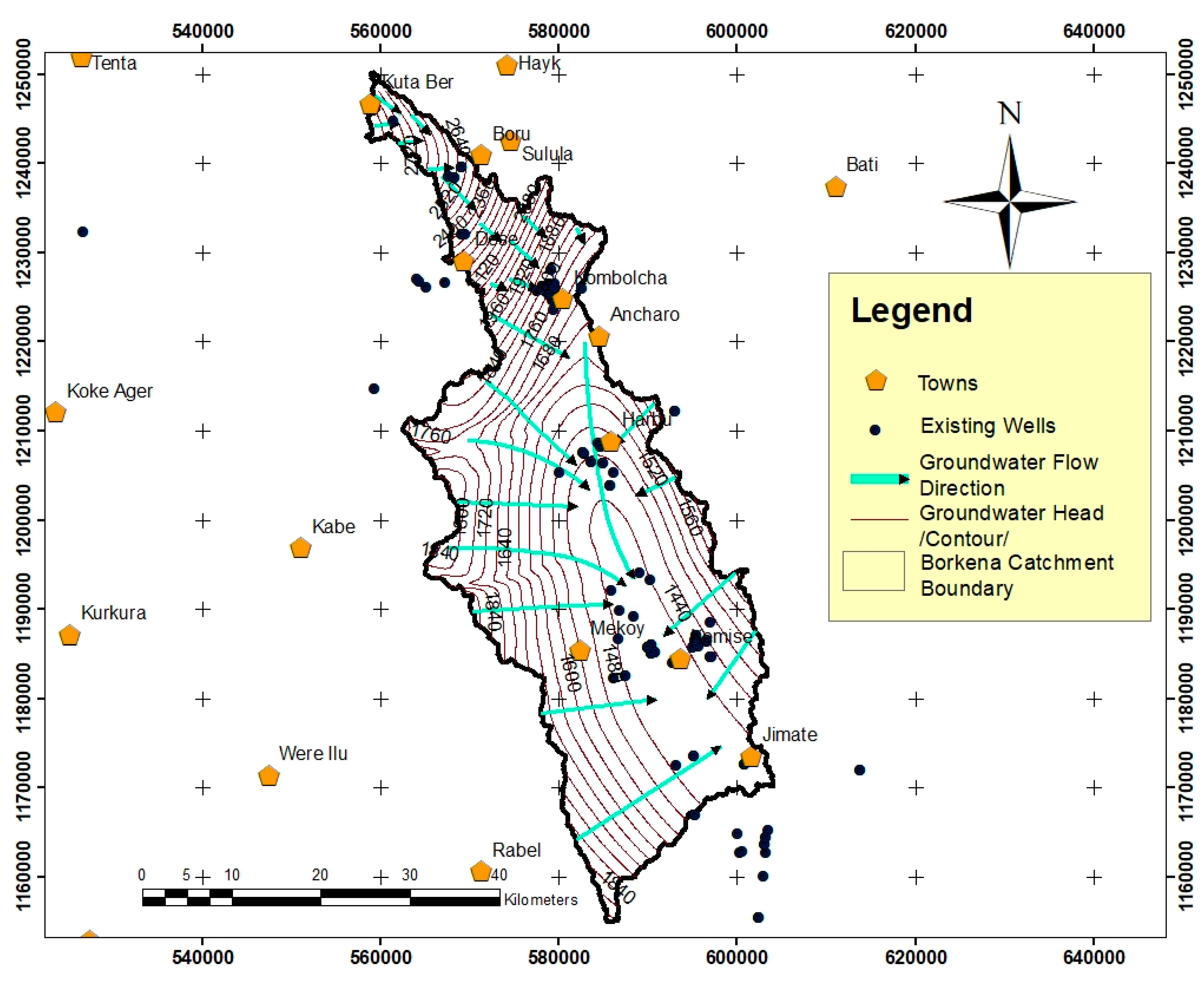
3.3. The Spatial Distribution of the Groundwater Head

The groundwater level and flow maps of the study area were produced using AutoCAD and ArcGIS software from existing borehole data. The groundwater level and contour maps showed that, generally, the groundwater flows from the tertiary volcanic aquifer at Kutaber toward the alluvial aquifer at Combolcha and Kemisse and then to Chefa Swamp (Figure 6). The groundwater movement is influenced by the elevation, geological structures, and faults in the study area. For example, the groundwater level was higher in the tertiary volcanic aquifer at Kutaber, Boru Sillasse, and Dessie relative to the alluvial aquifers at Combolcha and Chefa, as indicated in the hydrogeological map of the study area (Figure 2).

3.4. Inter-Basin Groundwater Transfer

Although the Gerado Catchment (Abbay basin) is located at a higher elevation and the Combolcha and Kemisse (Awash) aquifers are located at lower elevations, it was assumed that there was no inter-basin groundwater flow between the two basins due to the very low hydraulic conductivity of the tertiary volcanic rocks, but this study suggests that there is an inter-basin transfer of groundwater from the Abbay to the Awash basins. This was also confirmed by the results from the physicochemical analysis, which showed an HCO3 compound in all of the three deep boreholes, except for changes in chemical composition, which likely occur due to the evolution during the inter-basin transfer process. A piper diagram was used to identify the chemical relationships among the water samples from the different boreholes. The water type at Gerado/Abbay basin (KCVTW-01-19), Combolcha/Awash basin (KCVTW-02-19), and Kemisse/Awash basin were Na-HCO3, Mg-Ca-Na-HCO3, and Na-Ca-HCO3-SO4, respectively (Figure 7). Due to the geochemical process in the groundwater flow, the Na-HCO3 water type in the Gerado catchment was likely changed to the Mg-Ca-Na-HCO3 type when it reached the Combolcha Catchment and, subsequently, to Na-Ca-HCO3-SO4 as it reached the Kemisse Catchment.

4. Conclusions

This study applied the SWAT–MODFLOW modeling successfully to understand the hydrological processes and groundwater movement in the case study of the Borkena Catchment. The calibration and validation of the SWAT model provided satisfactory performance with a coefficient of determination (R2) and Nash–Sutcliffe efficiency (NSE) of more than 0.5. The groundwater data from the borehole and river topographic analysis helped to identify parts of the Borkena River that were gaining, losing, and both gaining and losing, which is useful for implementing sustainable water management and use practices. Furthermore, the outputs of the SWAT–MODFLOW helped to further understand the surface and groundwater interactions. Based on the deep borehole analysis and geochemical analysis (water type analysis), the results suggest that there could be an inter-basin groundwater flow from the Abbay basin (Gerado) to the Awash basin (Combolcha–Kemisse). However, an isotope analysis is recommended for future research to make a more conclusive statement. The presence of such regional groundwater flow into the inner tertiary volcanic aquifer in the semi-arid area is beneficial to the communities living in the downstream areas, since they may use the groundwater for domestic, municipal, and irrigation activities. Such a type of study helps to devise proper water management planning that ensures sustainable groundwater and surface water use. Therefore, these surface water–groundwater interaction investigation results are essential for adapting the climate variability in an arid region. Although the study is focused on a case study site of the Borkena Catchment, the methods used in this study can be applied to similar catchments to address the growing challenges of groundwater and surface water over extractions.

Supplementary Materials

The following supporting information can be downloaded at: https://www.mdpi.com/article/10.3390/hydrology10020042/s1.

Author Contributions

Conceptualization, W.J.G. and E.T.; methodology, W.J.G.; software, W.J.G.; validation, W.J.G., G.T.A., E.T. and G.Y.E.; formal analysis, W.J.G.; investigation, W.J.G.; resources, W.J.G., G.T.A. and E.T.; data curation, W.J.G.; writing—original draft preparation, W.J.G.; writing—review and editing, E.T., Y.T.D., H.K.B. and G.T.A.; visualization, W.J.G., G.T.A. and E.T.; supervision, E.T.; project administration, W.J.G.; funding acquisition, G.T.A. All authors have read and agreed to the published version of the manuscript.

Funding

Gebiaw T. Ayele received funding from Griffith Graduate Research School, the Australian Rivers Institute and School of Engineering and Built Environment, Griffith University, Queensland, Australia.

Data Availability Statement

Not applicable.

Acknowledgments

This study was made possible through material support on geology, boreholes, and completion reports and transportation facilities during field visits by the first author from the Ethiopian Construction Design and Supervision Corporation, Water and Energy Design and Supervision Works Sector (ECDSWC-WEDSWS). We are especially indebted to the Ethiopian National meteorological Agency (NMA) and Ministry of Water, Irrigation, and Electricity (MoIE), which kindly provided daily weather data and river flow data, respectively. We also acknowledge the Water and Land Resource Center of Addis Ababa University in the Water Security and Sustainable Development Hub project for the provision of biophysical data, research advice and guidance about the research work. Gebiaw T. Ayele acknowledges Griffith Graduate Research School, the Australian Rivers Institute and School of Engineering, Griffith University, Queensland, Australia.

Conflicts of Interest

The authors declare no conflict of interest.

References

  1. Sophocleous, M. Interactions between groundwater and surface water: The state of the science. Hydrogeol. J. 2002, 10, 52–67. [Google Scholar] [CrossRef]
  2. Winter, T.C.; Harvey, J.; Franke, O.; Alley, W. Ground Water and Surface Water: A Single Resource, Circular 1139; US Geological Survey: Grand Forks, ND, USA, 1998.
  3. Gleeson, T.; Richter, B. How much groundwater can we pump and protect environmental flows through time? Presumptive standards for conjunctive management of aquifers and rivers. River Res. Appl. 2018, 34, 83–92. [Google Scholar] [CrossRef]
  4. Stevenazzi, S.; Masetti, M.; Beretta, G.P. Groundwater vulnerability assessment: From overlay methods to statistical methods in the Lombardy Plain area. Acque Sotter. -Ital. J. Groundw. 2017, 6. [Google Scholar] [CrossRef]
  5. Li, M.; Liang, X.; Xiao, C.; Cao, Y. Quantitative evaluation of groundwater–Surface water interactions: Application of cumulative exchange fluxes method. Water 2020, 12, 259. [Google Scholar] [CrossRef]
  6. Malagò, A.; Pagliero, L.; Bouraoui, F.; Franchini, M. Comparing calibrated parameter sets of the SWAT model for the Scandinavian and Iberian peninsulas. Hydrol. Sci. J. 2015, 60, 949–967. [Google Scholar] [CrossRef]
  7. Anderson, M.; Woessner, W.; Hunt, R. Applied groundwater modeling: Simulation of flow and advective transport. J. Hydrol. 1992, 140, 393–395. [Google Scholar]
  8. Lewandowski, J.; Meinikmann, K.; Krause, S. Groundwater–surface water interactions: Recent advances and interdisciplinary challenges. Water 2020, 12, 296. [Google Scholar] [CrossRef]
  9. Arnold, J.G.; Srinivasan, R.; Muttiah, R.S.; Williams, J.R. Large area hydrologic modeling and assessment part I: Model development 1. J. Am. Water Resour. Assoc. 1998, 34, 73–89. [Google Scholar] [CrossRef]
  10. Arnold, J.G.; Moriasi, D.N.; Gassman, P.W.; Abbaspour, K.C.; White, M.J.; Srinivasan, R.; Santhi, C.; Harmel, R.; Van Griensven, A.; Van Liew, M.W. SWAT: Model use, calibration, and validation. Trans. ASABE 2012, 55, 1491–1508. [Google Scholar] [CrossRef]
  11. Langevin, C.D.; Hughes, J.D.; Banta, E.R.; Niswonger, R.G.; Panday, S.; Provost, A.M. Documentation for the MODFLOW 6 Groundwater Flow Model; No. 6-A55; US Geological Survey: Grand Forks, ND, USA, 2017.
  12. Namitha, M.; JS, D.K.; Sreelekshmi, H. Ground water flow modelling using visual modflow. J. Pharmacogn. Phytochem. 2019, 8, 2710–2714. [Google Scholar]
  13. Mohammed, M.; Ayalew, B. Modeling for Inter-Basin Groundwater Transfer Identification: The Case of Upper Rift Valley Lakes and Awash River Basins of Ethiopia. J. Water Resour. Prot. 2016, 8, 1222. [Google Scholar] [CrossRef]
  14. Wu, D.D.; Anagnostou, E.N.; Wang, G.; Moges, S.; Zampieri, M. Improving the surface-ground water interactions in the Community Land Model: Case study in the Blue Nile Basin. Water Resour. Res. 2014, 50, 8015–8033. [Google Scholar] [CrossRef] [Green Version]
  15. Taye, M.T.; Ebrahim, G.Y.; Nigussie, L.; Hagos, F.; Uhlenbrook, S.; Schmitter, P. Integrated water availability modelling to assess sustainable agricultural intensification options in the Meki catchment, Central Rift Valley, Ethiopia. Hydrol. Sci. J. 2022, 67, 2271–2293. [Google Scholar] [CrossRef]
  16. Walter, M.T.; Shaw, S.B.; Garen, D.C.; Moore, D.S. “Curve Number Hydrology in Water Quality Modeling: Uses, Abuses, and Future Directions,” by David C. Garen and Daniel S. Moore. J. Am. Water Resour. Assoc. 2005, 41, 1491. [Google Scholar] [CrossRef]
  17. Neitsch, S.L.; Arnold, J.G.; Kiniry, J.R.; Williams, J.R. Soil and Water Assessment Tool Theoretical Documentation; Version 2005; USDA-ARS Grassland, Soil and Water Research Laboratory: Temple, TX, USA, 2005. Available online: www.brc.tamus.edu/swat/doc.html (accessed on 15 January 2020).
  18. Daggupati, P.; Pai, N.; Ale, S.; Douglas-Mankin, K.R.; Zeckoski, R.W.; Jeong, J.; Parajuli, P.B.; Saraswat, D.; Youssef, M.A. A recommended calibration and validation strategy for hydrologic and water quality models. Trans. ASABE 2015, 58, 1705–1719. [Google Scholar]
  19. Abbaspour, K.C.; Yang, J.; Maximov, I.; Siber, R.; Bogner, K.; Mieleitner, J.; Zobrist, J.; Srinivasan, R. Modelling hydrology and water quality in the pre-alpine/alpine Thur watershed using SWAT. J. Hydrol. 2007, 333, 413–430. [Google Scholar] [CrossRef]
  20. Yang, J.; Reichert, P.; Abbaspour, K.C.; Xia, J.; Yang, H. Comparing uncertainty analysis techniques for a SWAT application to the Chaohe Basin in China. J. Hydrol. 2008, 358, 1–23. [Google Scholar] [CrossRef]
  21. Mathevet, T.; Michel, C.; Andréassian, V.; Perrin, C. A bounded version of the Nash-Sutcliffe criterion for better model assessment on large sets of basins. IAHS Publ. 2006, 307, 211. [Google Scholar]
  22. Moriasi, D.N.; Arnold, J.G.; Van Liew, M.W.; Bingner, R.L.; Harmel, R.D.; Veith, T.L. Model evaluation guidelines for systematic quantification of accuracy in watershed simulations. Trans. ASABE 2007, 50, 885–900. [Google Scholar] [CrossRef]
  23. ECDSWC-WEDSWS. Ethiopian Construction Design and Supervision Works Corporation, Water and Energy Design and Supervision Works Sector (ECDSWC-WEDSWS) Kobo-Chefa Groundwater Evaluation Report. V. III. 2019; Unpublished. [Google Scholar]
  24. ECDSWC-WEDSWS. Ethiopian Construction Design and Supervision Works Corporation, Water and Energy Design and Supervision Works Sector (ECDSWC-WEDSWS) (KCVTW-01-19) Well Completion Report. V. I. 2020; Unpublished. [Google Scholar]
  25. ECDSWC-WEDSWS. Ethiopian Construction Design and Supervision Works Corporation, Water and Energy Design and Supervision Works Sector (ECDSWC-WEDSWS) (KCVTW-02-19) Well Completion Report. V. II. 2020; Unpublished. [Google Scholar]
  26. ECDSWC-WEDSWS. ECDSWC-WEDSWS. Ethiopian Construction Design and Supervision Works Corporation, Water and Energy Design and Supervision Works Sector (ECDSWC-WEDSWS) (KCVTW-03-19) Well Completion Report. V. III. 2020; Unpublished. [Google Scholar]
  27. Freeze, R.A.; Cherry, J.A. Groundwater; Prentice-Hall Inc.: Eaglewood Cliffs, NJ, USA, 1979. [Google Scholar]
  28. Wilson, C.P. Groundwater Hydrology, 2nd ed.; Todd, D.K., Ed.; Wiley: New York, NY, USA, 1980; p. 552. ISBN 0 471 08641 X. [Google Scholar]
  29. Todd, D.K.; Mays, L.W. Groundwater Hydrology; John Wiley & Sons: Hoboken, NJ, USA, 2004. [Google Scholar]
  30. Unnikrishnan, M.; Sarda, V.K. Streambed Hydraulic conductivity: A state of art. Int. J. Mod. Trends Eng. Res. 2016, 3, 209–217. [Google Scholar]
  31. Bailey, R.T.; Wible, T.C.; Arabi, M.; Records, R.M.; Ditty, J. Assessing regional-scale spatio-temporal patterns of groundwater–surface water interactions using a coupled SWAT-MODFLOW model. Hydrol. Process. 2016, 30, 4420–4433. [Google Scholar] [CrossRef]
  32. Bailey, R.; Park, S. SWAT-MODFLOW Tutorial Version 3 Documentation for Preparing and Running SWAT-MODFLOW Simulations; Department of Civil and Environmental Engineering, Colorado State University: Fort Collins, CO, USA, 2019. [Google Scholar]
  33. Chernet, T. Hydrogeological Map of Ethiopia, 1:2.000.000; Ethiopian Institute of Geological Surveys: Addis Ababa, Ethiopia, 1988. [Google Scholar]
  34. Kebede, S. Groundwater in Ethiopia: Features, Numbers and Opportunities; Springer: Berlin/Heidelberg, Germany, 2012. [Google Scholar]
  35. Gidafie, D.; Tafesse, N.; Hagos, M. Estimation of Groundwater Recharge Using Water Balance Model: A Case Study in the Gerado Basin, North Central Ethiopia. Int. J. Earth Sci. Eng. 2016, 9, 942–950. [Google Scholar]
  36. Mechal, A.; Birk, S.; Dietzel, M.; Leis, A.; Winkler, G.; Mogessie, A.; Kebede, S. Groundwater flow dynamics in the complex aquifer system of Gidabo River Basin (Ethiopian Rift): A multi-proxy approach. Hydrogeol. J. 2017, 25, 519–538. [Google Scholar] [CrossRef] [Green Version]
Figure 1. Location map of Borkena Catchment.
Hydrology 10 00042 g001
Figure 2. A hydrogeological map of the study area produced (data source: ECDSWC-WEDSWS).
Hydrology 10 00042 g002
Figure 3. Monthly observed and simulated stream flow: (a) Calibration period, (b) validation period.
Hydrology 10 00042 g003
Figure 4. Gerado–Combolcha cross-section showing the regional and local groundwater flow produced.
Hydrology 10 00042 g004
Figure 5. Kutaber–Combolcha to Kemisse cross-section showing the local groundwater flow.
Hydrology 10 00042 g005
Figure 6. Groundwater contour and flow map of the study area.
Hydrology 10 00042 g006
Figure 7. Piper plot diagram showing the water types of the existing three boreholes, produced using acquacheme software (data source: ECDSWC-WEDSWS).
Hydrology 10 00042 g007
Table 1. Land use/land cover classes in the study catchment (source: Ministry of Water and Energy (MoWE)).
Land Use/CoverArea (km2)Area (%)
Agricultural796.0449.57
Rangeland237.3414.78
Brushland29718.49
Plantation Forest19.91.24
Bare Land/Barren160.319.98
Natural Forest0.170.01
Deciduous Forest/Wood0.010
Wetlands95.235.93
Total1606100
Table 2. Major soil types in Borkena Catchment (source: Ministry of Water and Energy (MoWE)).
ValueSOIL_IDArea (km2)Area (%)
1Lithic Leptosols886.6755.21
2Eutric Vertisols302.0918.81
3Eutric Leptosols262.2616.33
4Vertic Vertisol154.989.65
Total1606100
Table 3. Fitted values of calibrated flow parameters with absolute t-stat and p-value for the SWAT model.
Parameter NameDescriptionRangeFitted Valuest-Statp-Value
SOL_AWCSoil available water capacity (mm H2O)±25%0.070.020.98
CN2Curve number for moisture condition II±25%33.820.540.61
GWQMNThreshold depth of water in the shallow aquifer (mm H2O)0–5000−29.24−0.550.61
GW_DELAYGroundwater delay (days)0–50028.85−0.650.55
ESCOSoil evaporation compensation factor0.5–0.113.560.880.42
ALPHA_BFBaseflow alpha factor (1/days)0–10.60−1.240.27
REVAPMNThreshold depth of water in the shallow aquifer for “revap” or “percolation” to the deep aquifer to occur (mm H2O)0–50062.291.650.16
GW_REVAPGroundwater “revap” coefficient0.02–0.2−0.057−1.820.13
RCHRG_DPDeep aquifer percolation fraction0–5000.206−2.350.07
Table 4. Table showing the default values before calibration and the calibration and validation statistics for the monthly observed and simulated stream flow.
ParameterDefault ValueCalibrated (2000–2007)Validated (2008–2014)
R20.330.680.64
NSE0.330.660.63
PBIAS−3.90%−2.70%2.48%
Table 5. Average long-term annual water balance of the calibrated SWAT model in the study catchment.
ParameterValues (mm)% of Annual Rainfall
Precipitation1017.5
Surface Runoff Discharge out of the Total Flow241.5423
Lateral flow Soil Discharge out of the Total Flow67.316.6
Groundwater (Shallow Aquifer) Contribution to Stream Flow79.427.8
Groundwater (Deep Aquifer) Flow5.710.56
REVAP (Shallow Aquifer = Soil/Plants)29.99
Deep Aquifer Recharge5.7412
Total Aquifer Recharge114.75
Total Water Yield393.9938.7
Percolation out of Soil114.7611.2
Actual Evapotranspiration594.558.4
Potential Evapotranspiration1621
Table 6. Average long-term (1979–2017) monthly water balance estimates of the SWAT–MODFLOW model in the study area.
MONTHPREC (mm)SURQ (mm)LATQ (mm)GWQ (mm)PERCOLATE (mm)SW (mm)ET (mm)PET (mm)WATER YIELD (mm)
Jan.14.000.370.770.000.0029.2514.77174.822.00
Feb.0.300.000.090.000.0027.5610.99105.070.67
Mar.5.400.000.060.000.0024.4320.98160.870.55
Apr.149.8010.026.750.002.1877.8773.72141.2616.91
May4.400.003.580.040.4955.0526.59107.844.12
Jun.111.7018.356.810.644.9082.5952.97139.3726.02
Jul.236.1589.7613.314.3647.93123.79109.86161.39106.94
Aug.287.0092.2916.7317.8579.41123.1295.17125.16116.23
Sept.103.4013.7711.5338.5929.97106.1168.79118.3754.62
Oct.54.408.003.8835.721.0797.2051.20123.0734.03
Nov.51.208.983.0316.350.3892.9544.28134.0028.67
Dec.0.000.000.771.440.0067.7625.18129.783.23
Table 7. Aquifer parameter values calculated using Aquifer Test software, from existing boreholes’ raw data (Source ECDSWC-WEDSWS).
No.ParameterWell ID
KCTVW-01-19 (GERADO)KCTVW-02-19 (COMBOLCHA)KCTVW-03-19 (KEMISSE)
1Hydraulic Conductivity (Hk, m/d)9.099.329.41
2Transmissivity (T, m2/d)9559781030
3Static Water Level (m)0 (artesian)10.240 (artesian)
4Discharge (Q, l/s)8075.575
5Depth (m)500600512
6Surface Elevation (m)228218501444
7AquifersAlluvial Deposit; Weathered and Fractured Basalt and RhyoliteAlluvial Deposit; Moderately Weathered and Fractured BasaltAlluvial Deposit with Highly fractured Basalt
8Casing Designed0–230 m cased with blind steel casing and grouted with cement to isolate alluvial aquifer from the basaltic aquifer0–251 m cased with blind and grouted with cement to isolate the alluvial aquifer from the basaltic aquiferCased with screen and blind casing from top to bottom both the alluvial and basaltic aquifers
Disclaimer/Publisher’s Note: The statements, opinions and data contained in all publications are solely those of the individual author(s) and contributor(s) and not of MDPI and/or the editor(s). MDPI and/or the editor(s) disclaim responsibility for any injury to people or property resulting from any ideas, methods, instructions or products referred to in the content.

