

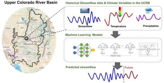
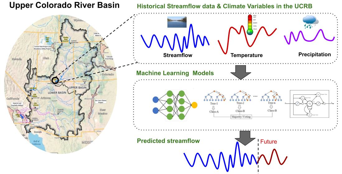
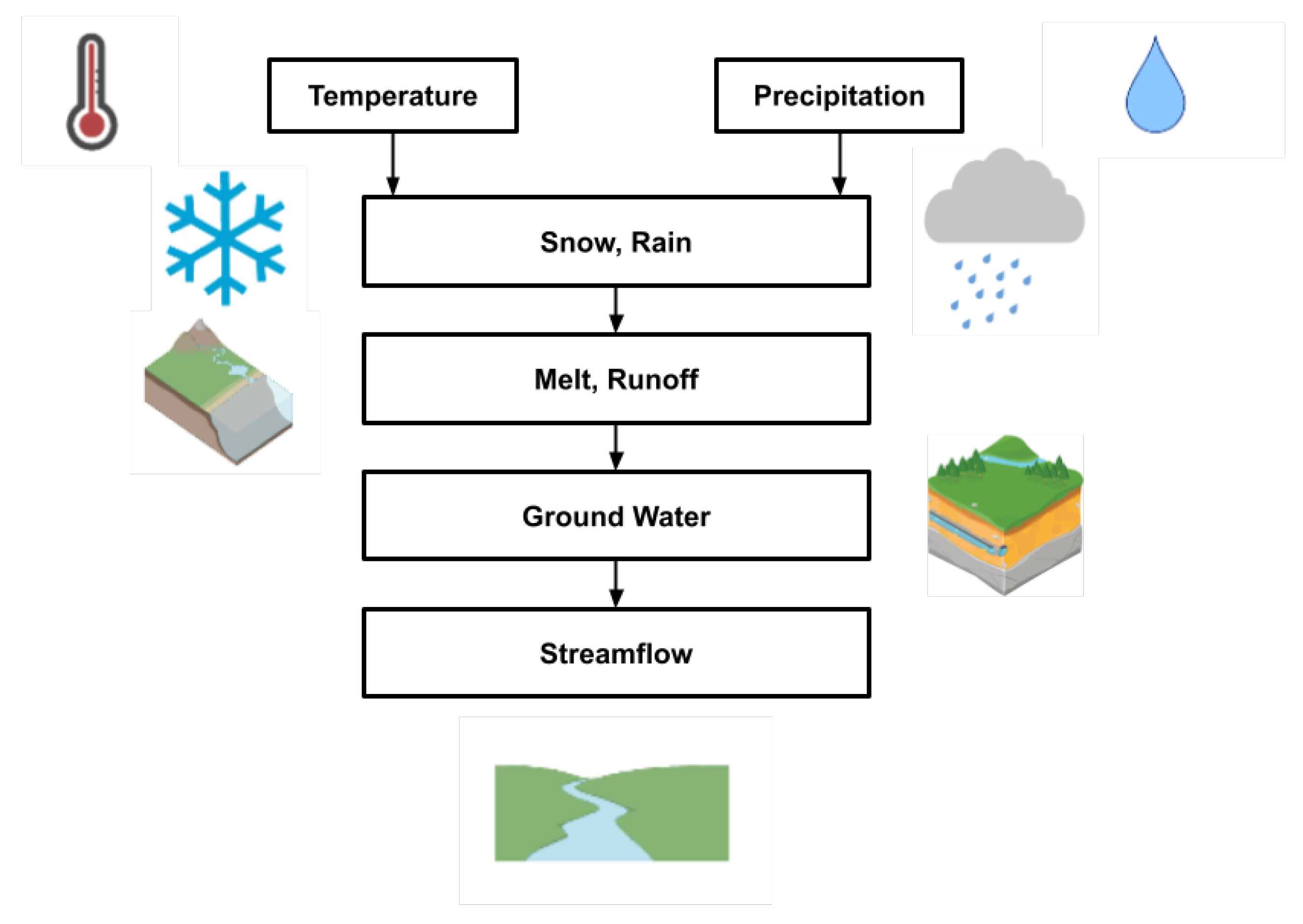
ML-Based Streamflow Prediction in the Upper Colorado River Basin Using Climate Variables Time Series Data


Abstract
:
1. Introduction
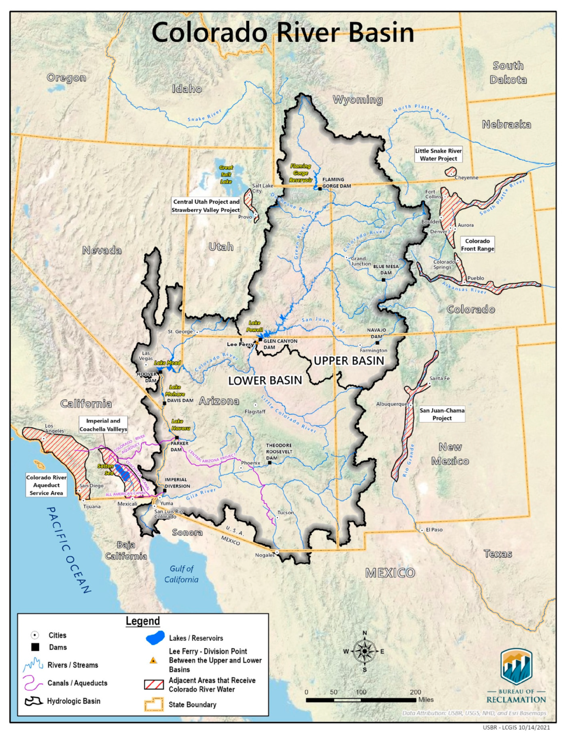
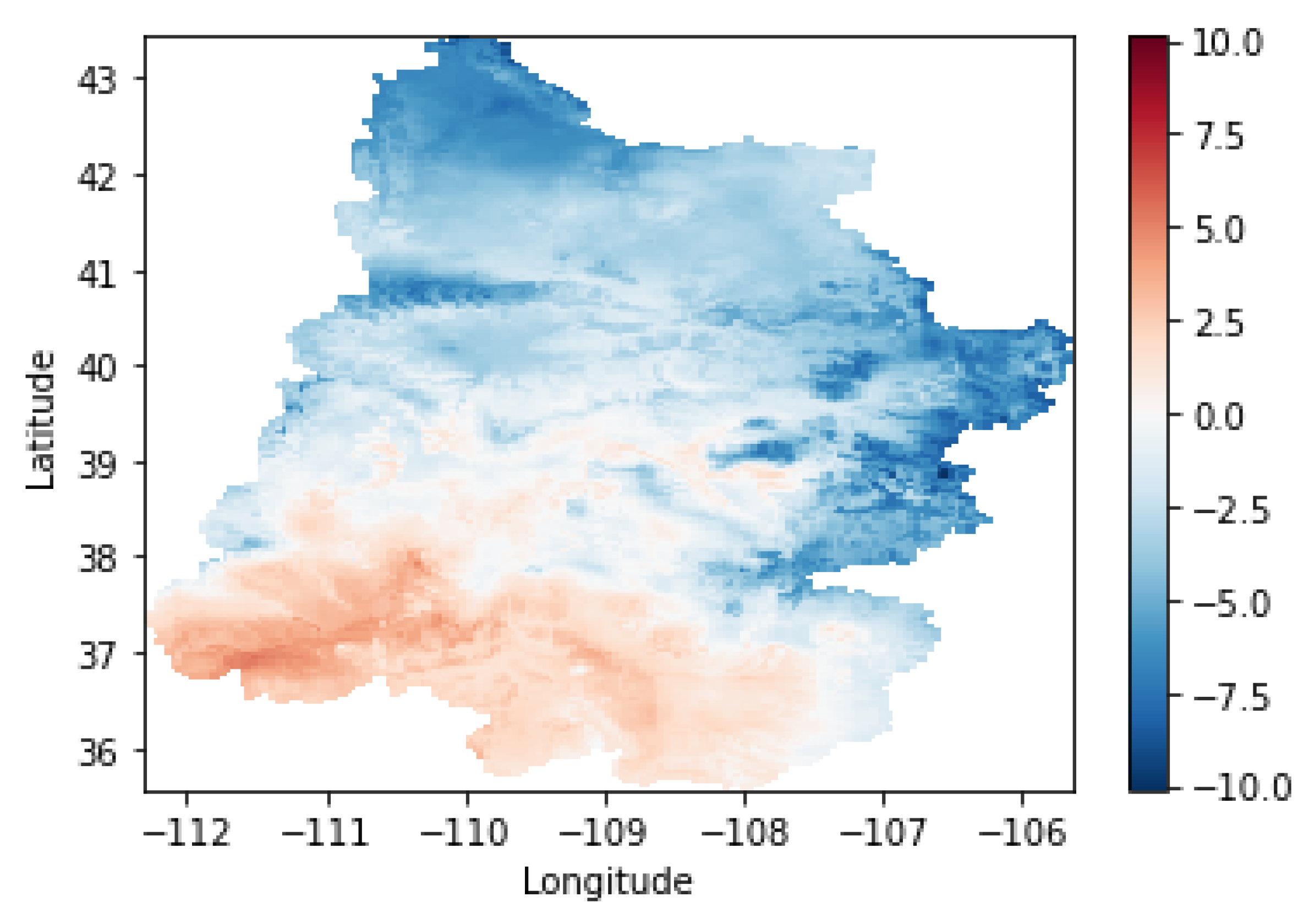
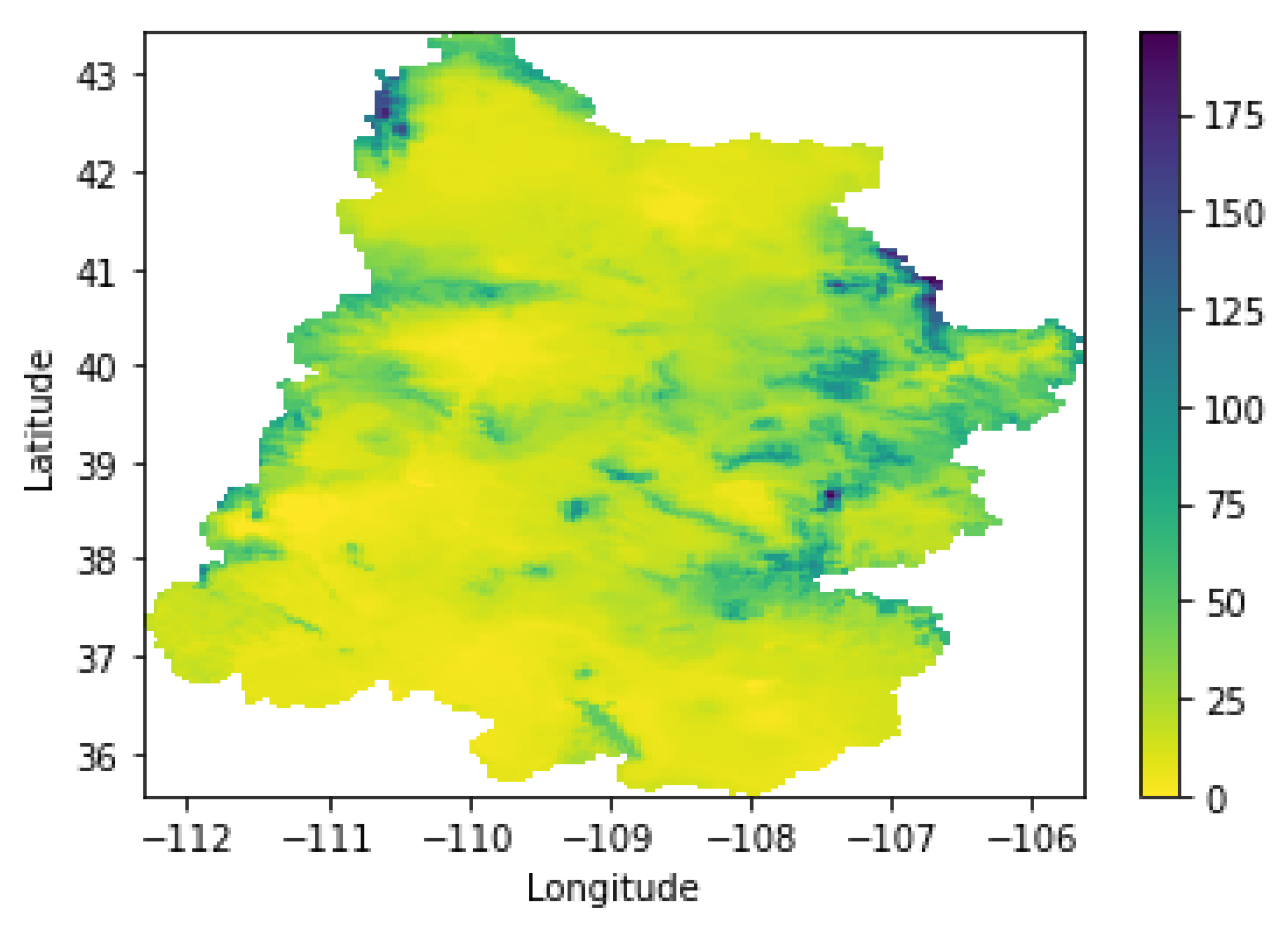
2. Study Site
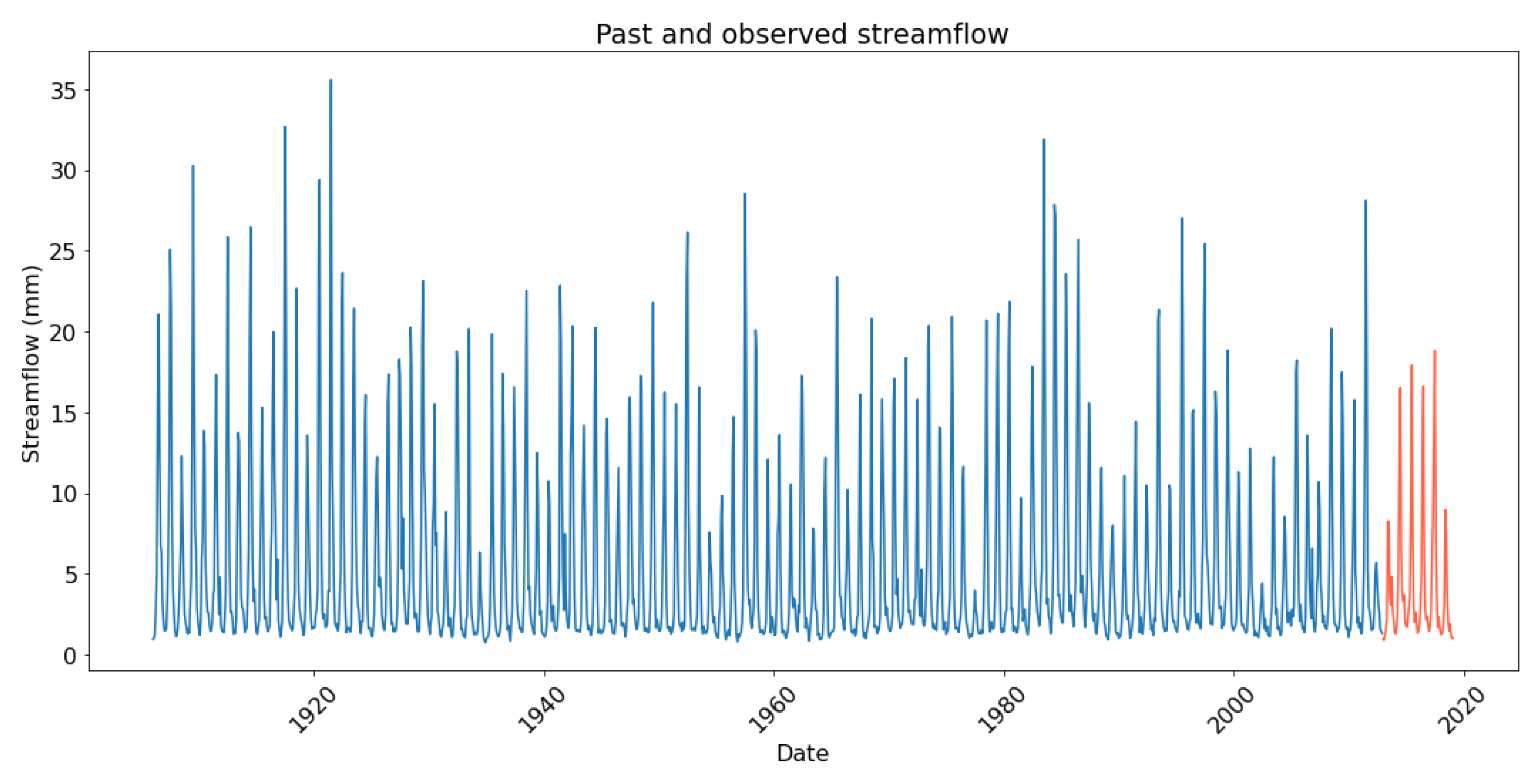
3. Data
4. Methodology
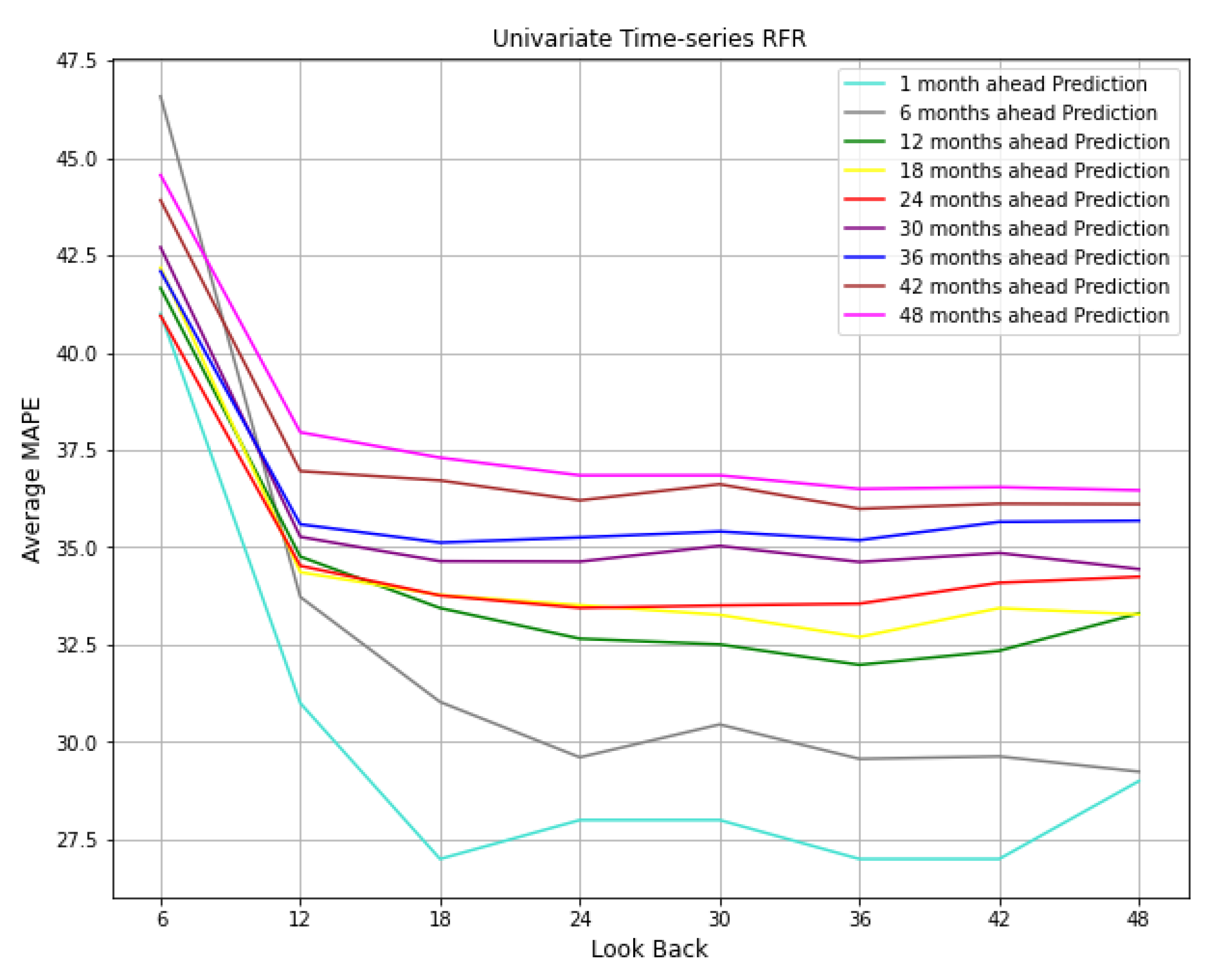
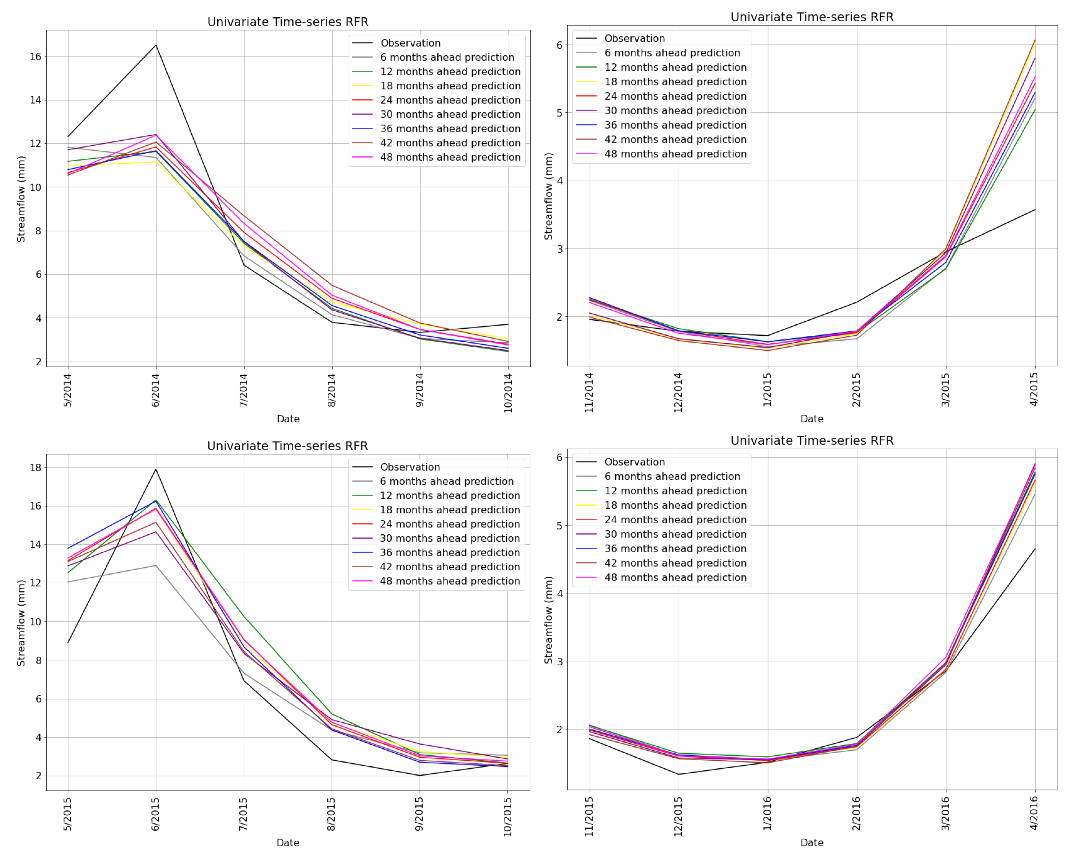
4.1. Univariate Time-Series Prediction Model
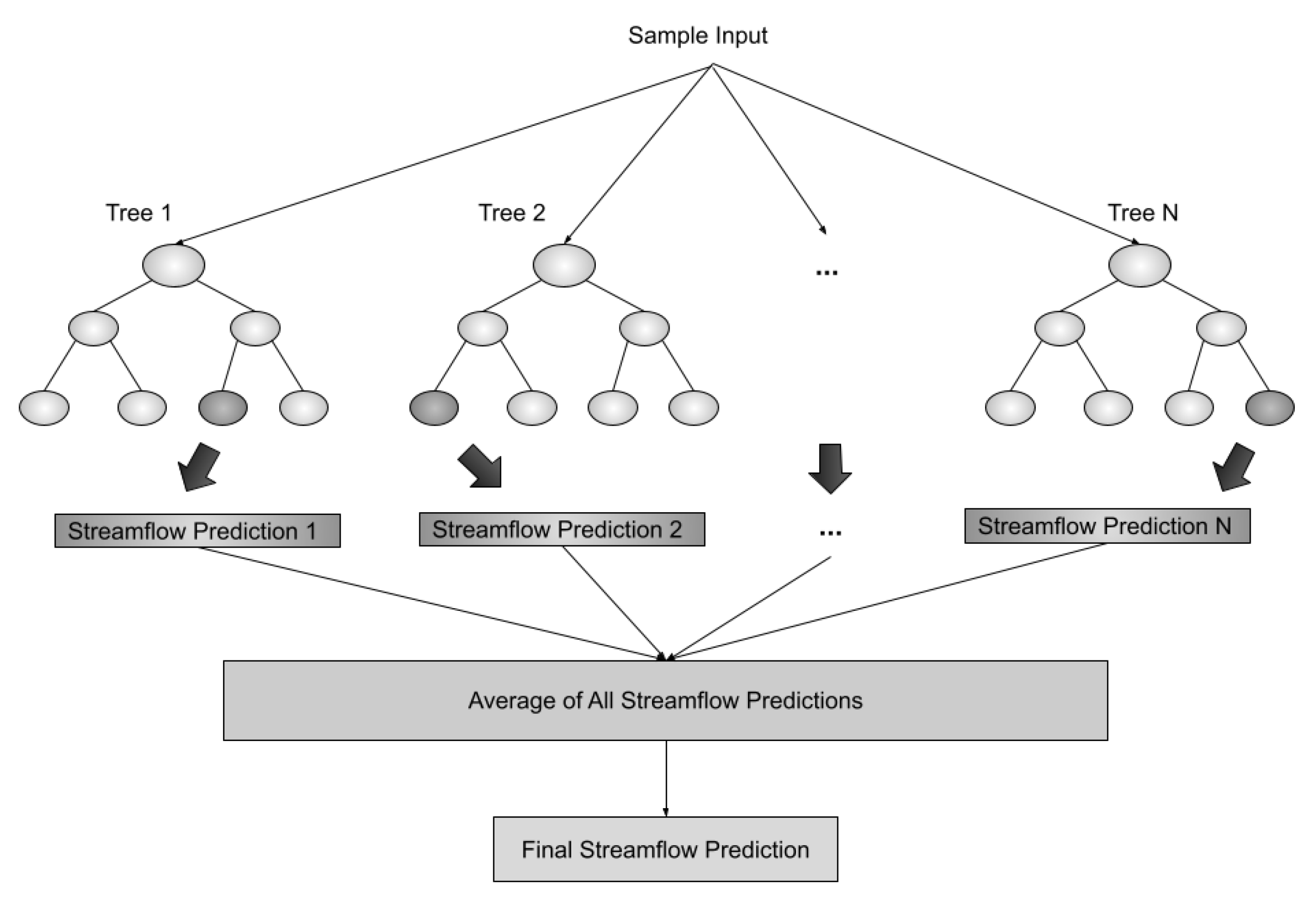
4.1.1. RFR
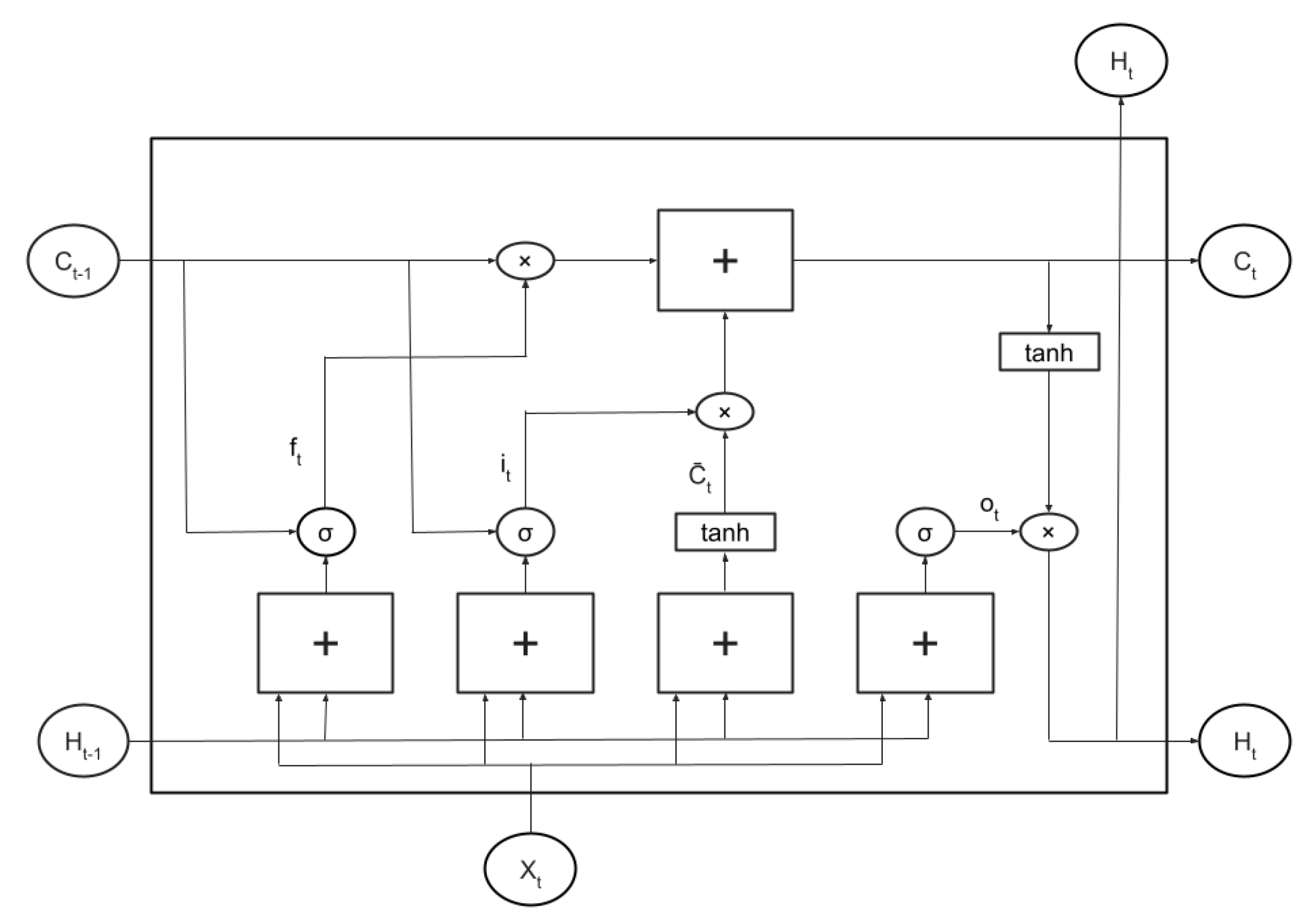
4.1.2. LSTM
4.1.3. SARIMA
4.1.4. PROPHET
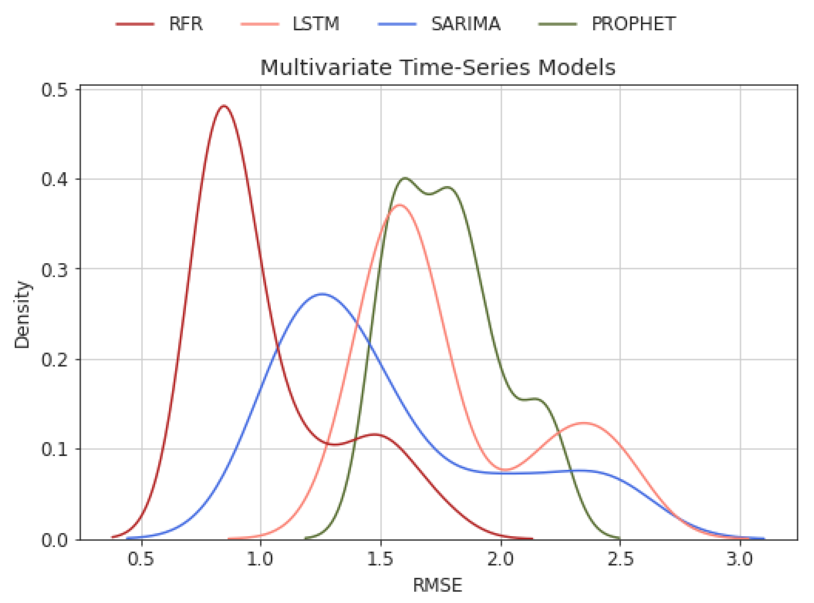
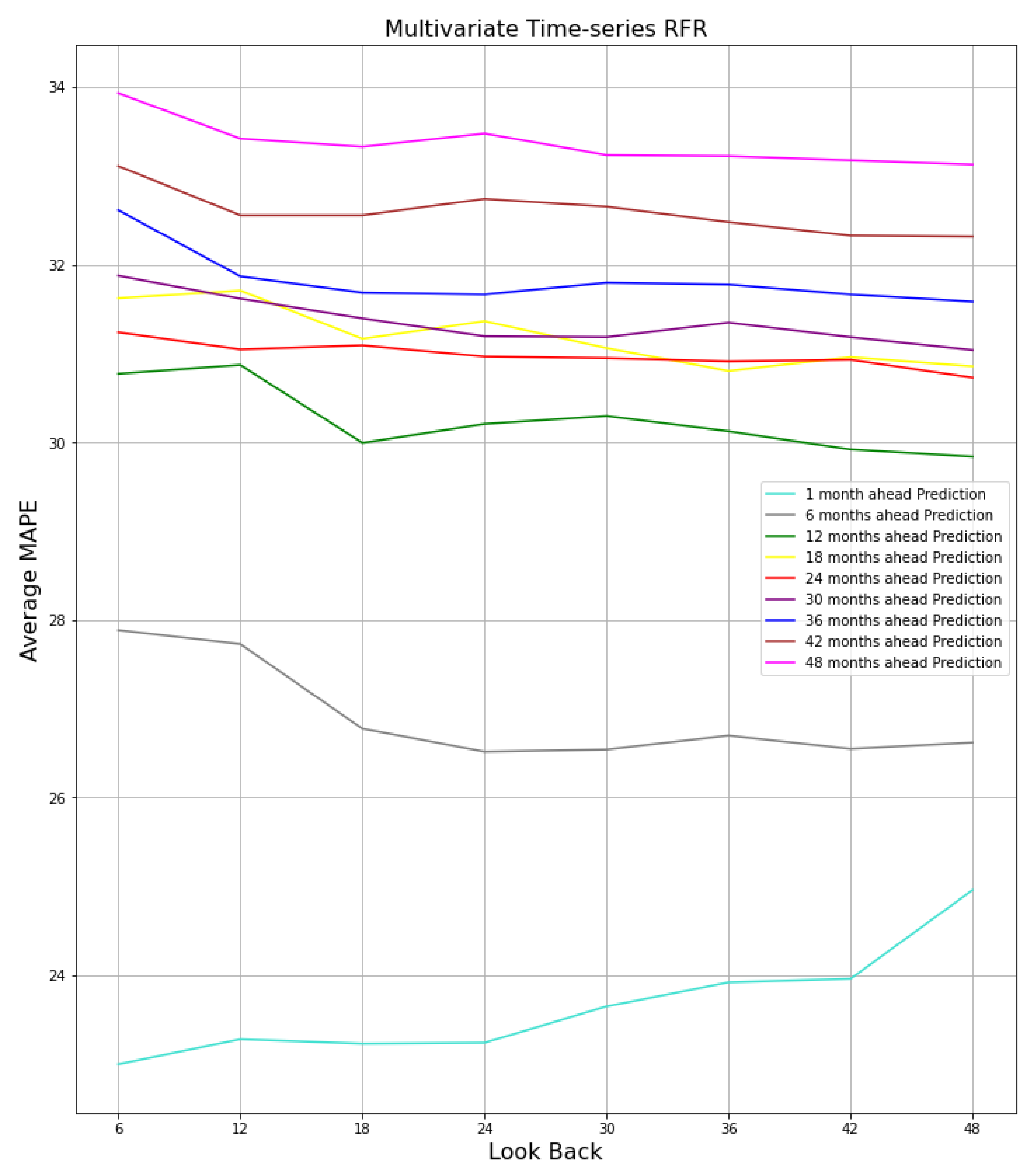
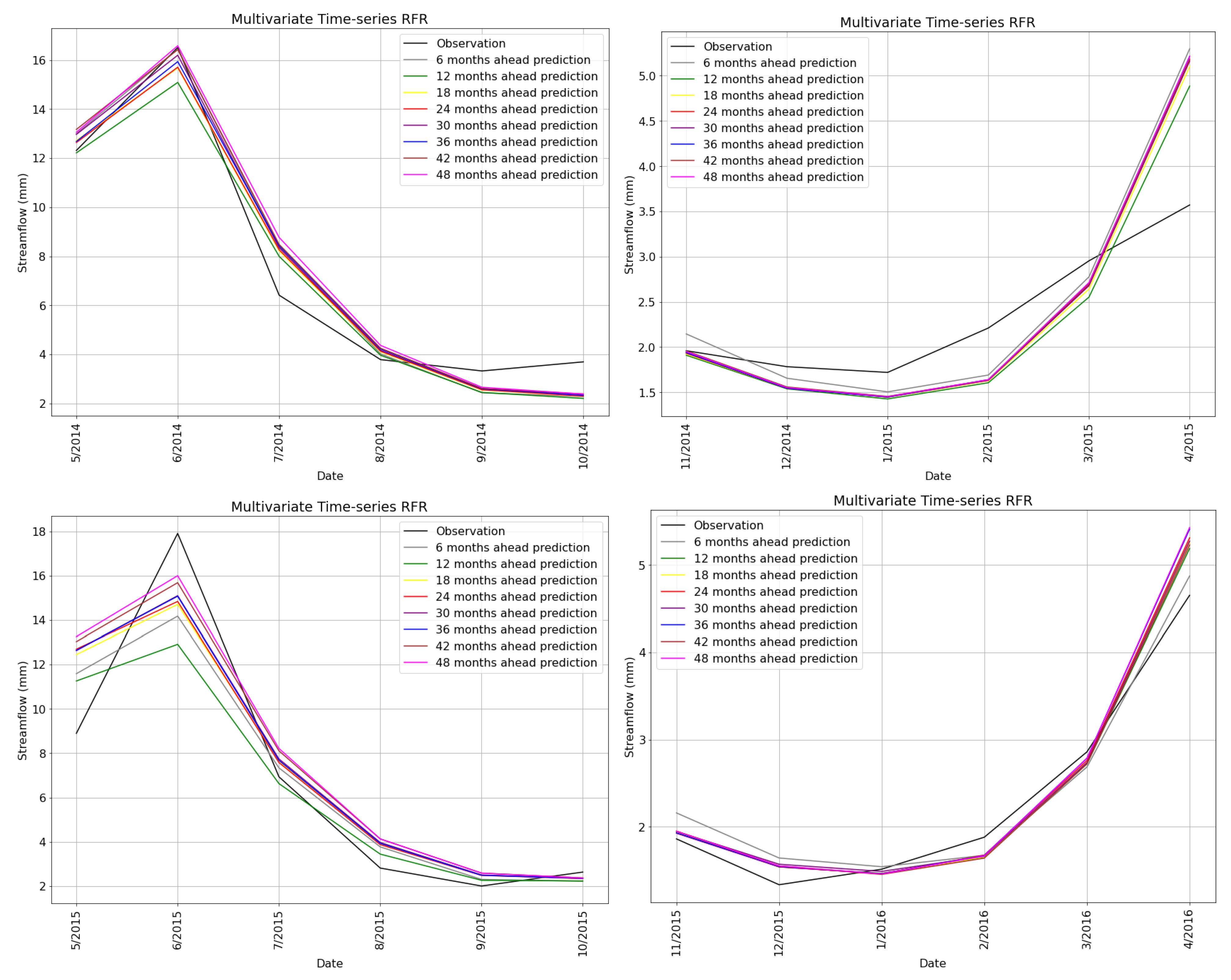
4.2. Multivariate Time-Series Model Prediction
- RFR: RFR’s input sequence is tripled in which the first 24 elements represent the discharge values, the second 24 elements represent the temperature values, and the last 24 elements represent the precipitation values.
- LSTM: LSTM’s input is a 2-dimensional matrix of shape (72, 3). The first dimension represents the number of elements, and the latter represents the three features, i.e., discharge, temperature, and precipitation.
- SARIMAX: Since we added extra features to the model, SARIMAX has been used instead of SARIMA. The exogenous factor of SARIMAX allows us to forecast future streamflow using external factors such as temperature and precipitation [75,76]. SARIMAX, as a seasonal auto-regressive integrated moving average model with exogenous factors, is defined as:
- PROPHET: Two additional regressors have been added to consider temperature and precipitation for the PROPHET model.
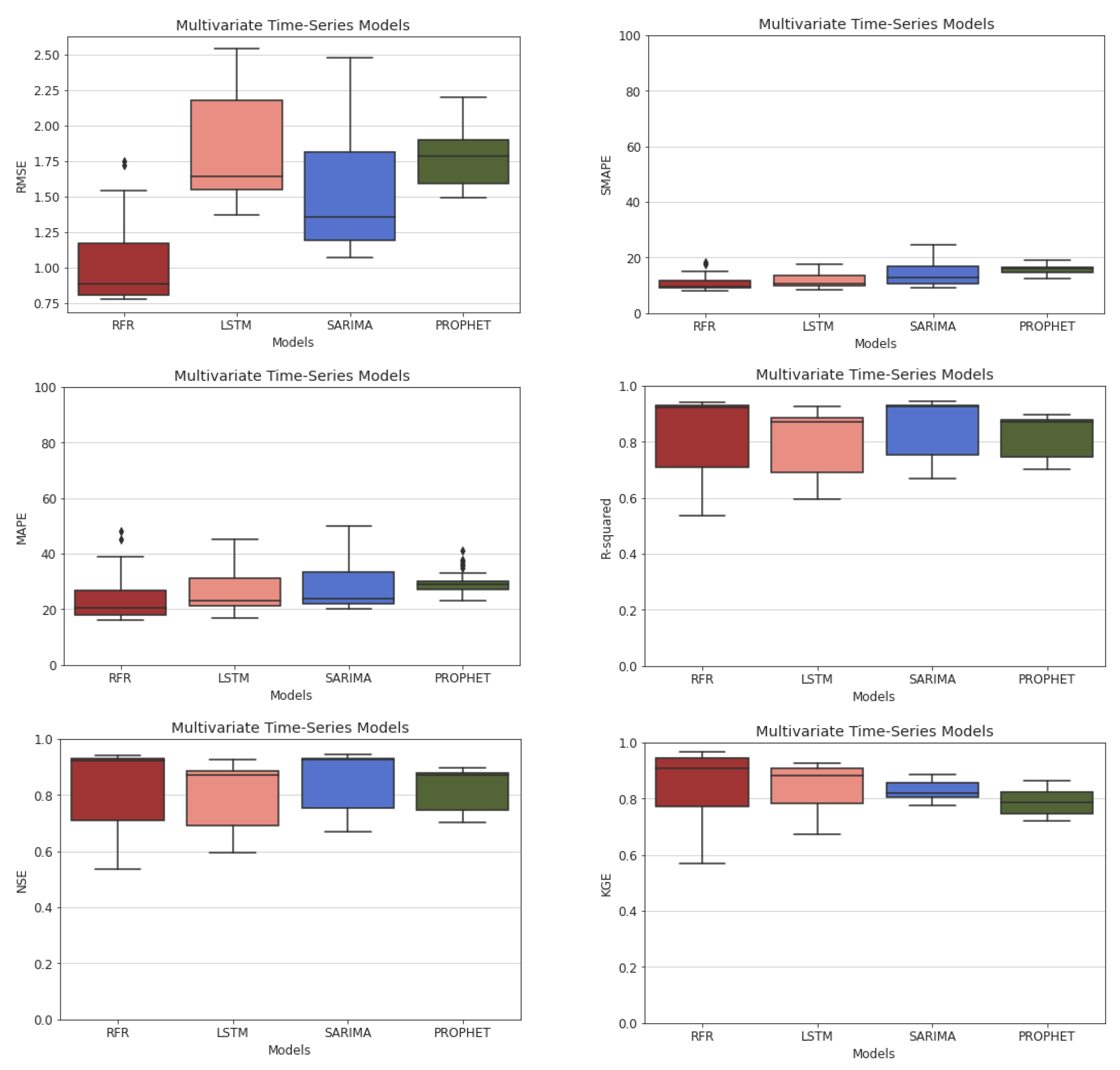
4.3. Evaluation Metrics
- Root Mean Square Error (RMSE): RMSE is widely used in regression-based prediction tasks, and it quantifies the closeness between predictions and observations. RMSE is defined as follows:
- R-squared (): R-squared metric, as a coefficient of determination, is used to measure how the prediction is aligned with the observation. is defined as:where RSS is the sum of the squared residuals, and TSS is the total sum of squares. The closer the value of R-squared to 1, the better the model’s predictions compared to the actual values.
- Mean Absolute Percentage Error (MAPE): MAPE is one of the most widely used metrics in the literature, and is defined as:
- Kling–Gupta efficiency (KGE): We use KGE, which is a revised version of NSE [79]. KGE is defined as below:
5. Experimental Results
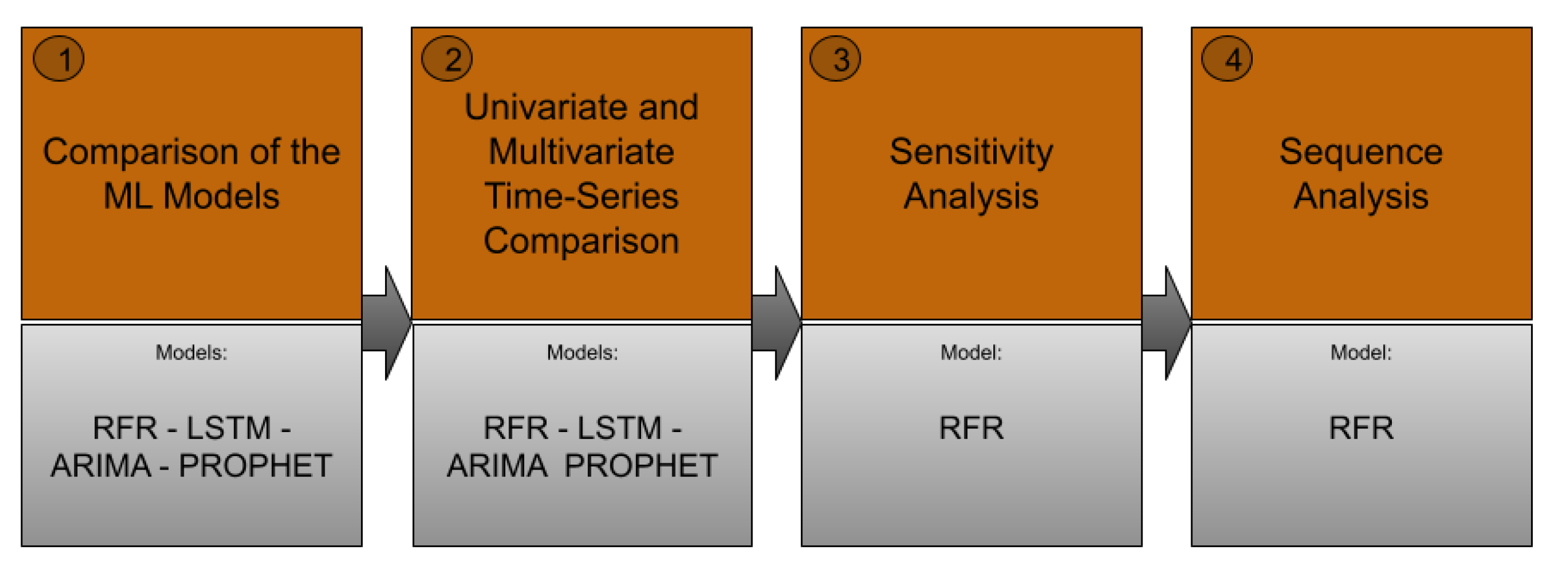
5.1. Comparison of the ML Models
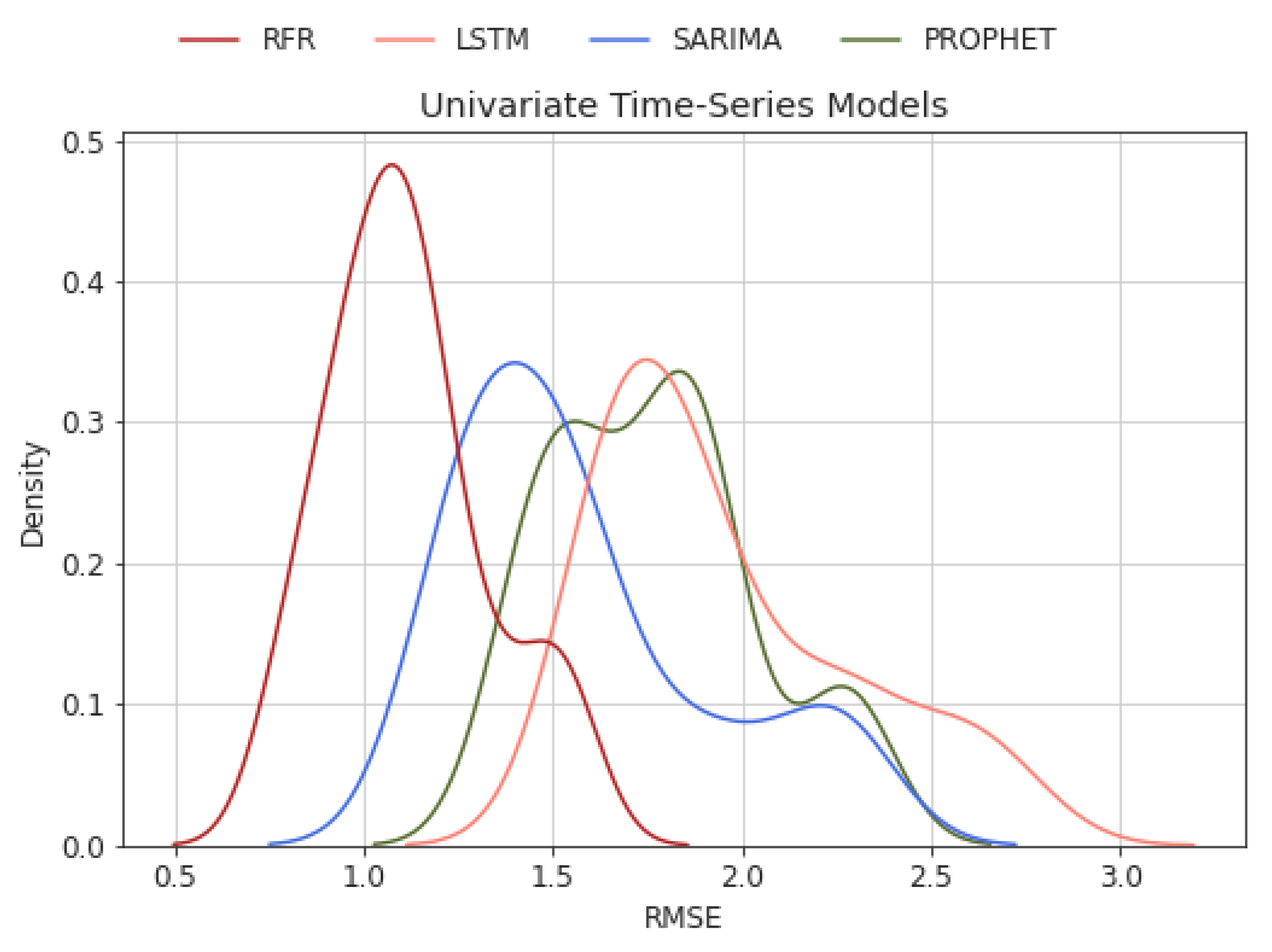
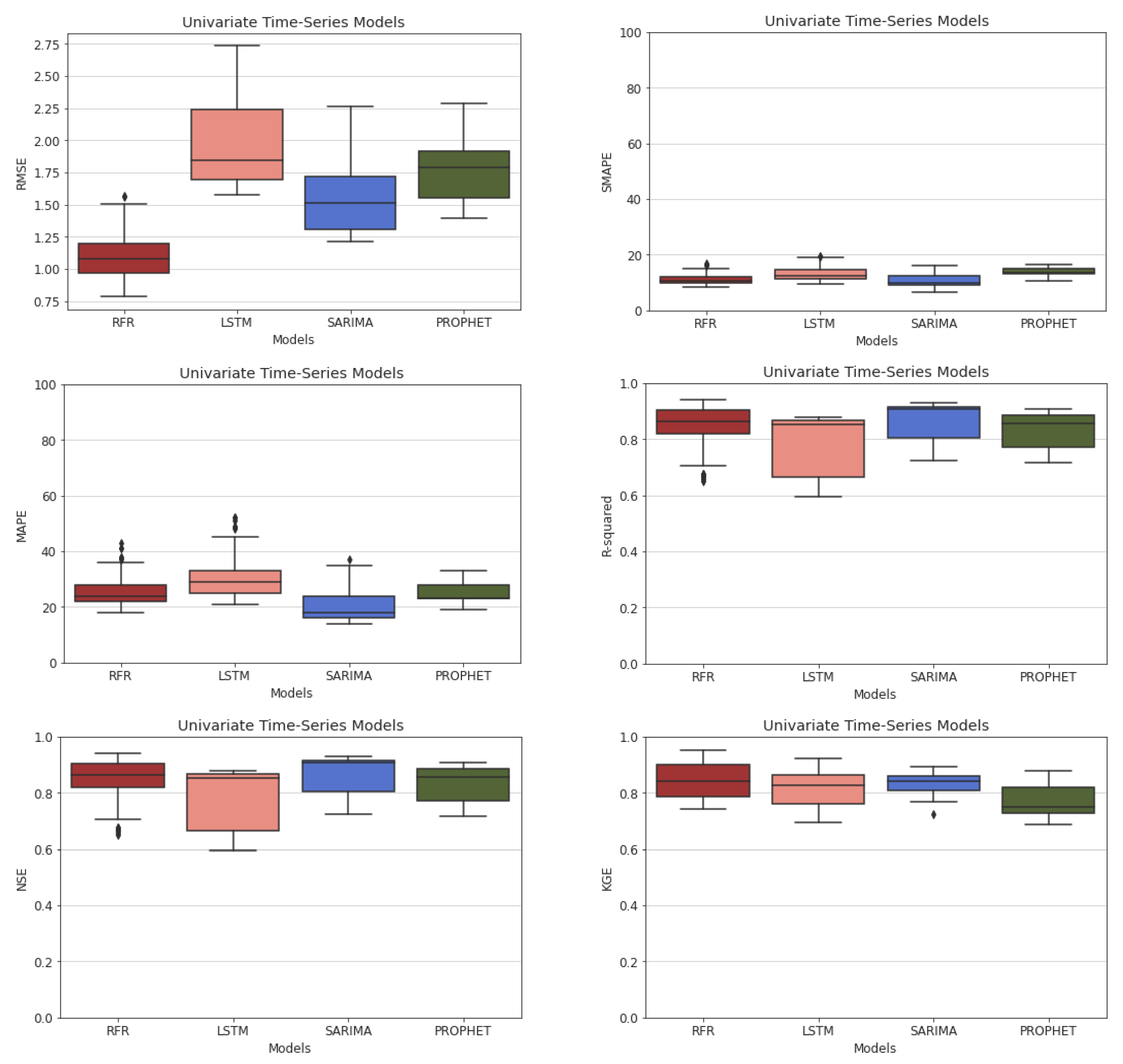
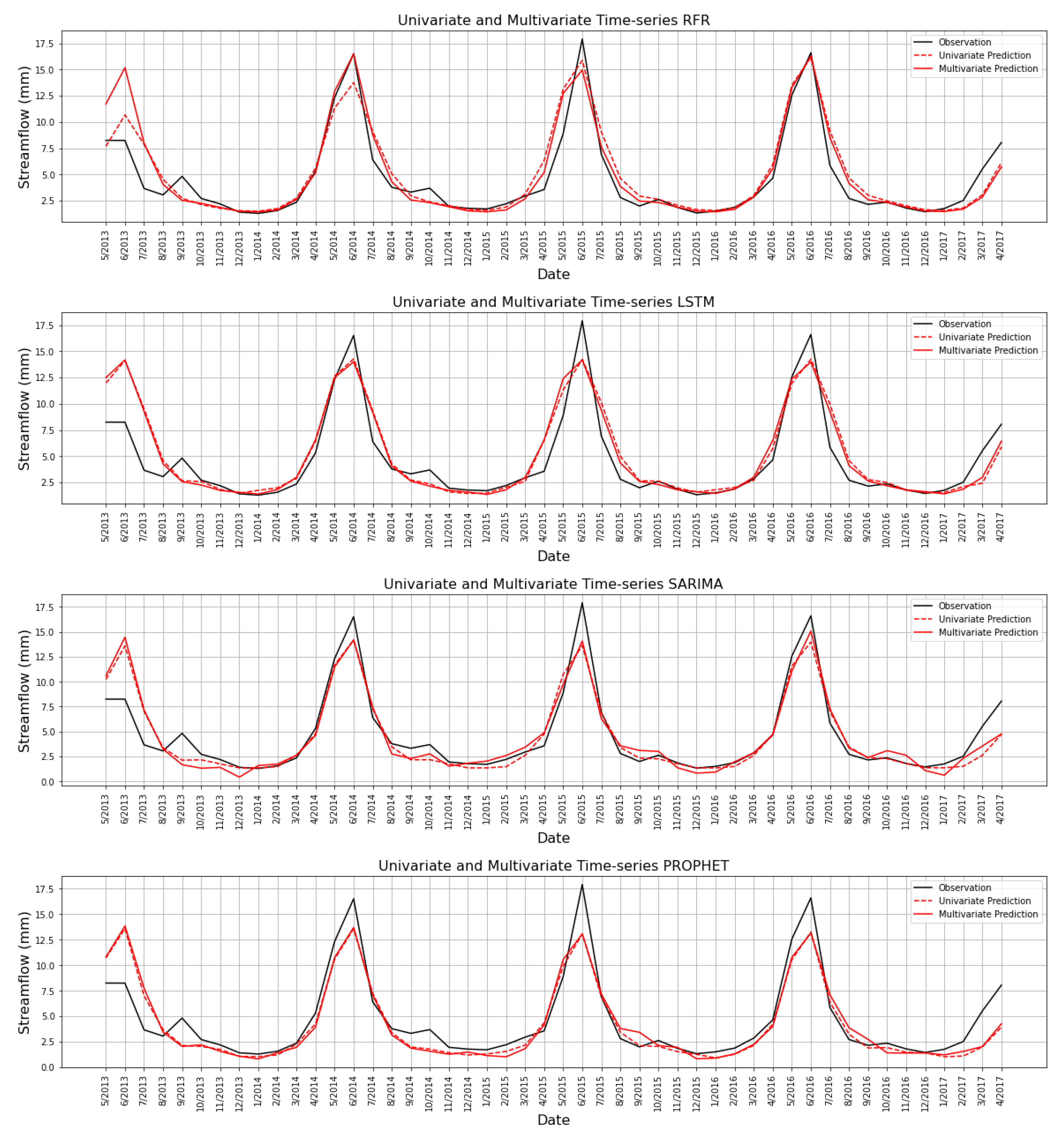
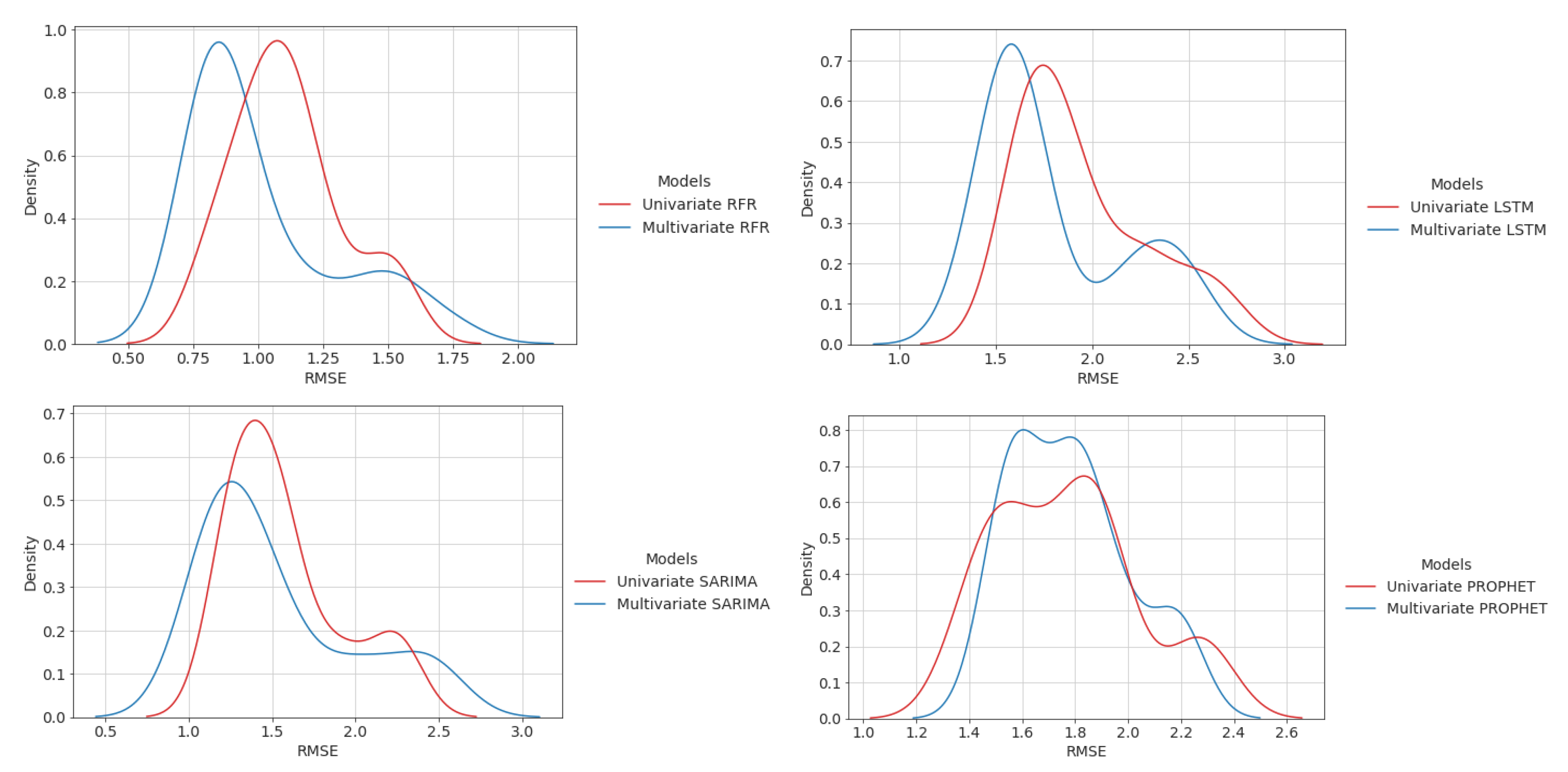
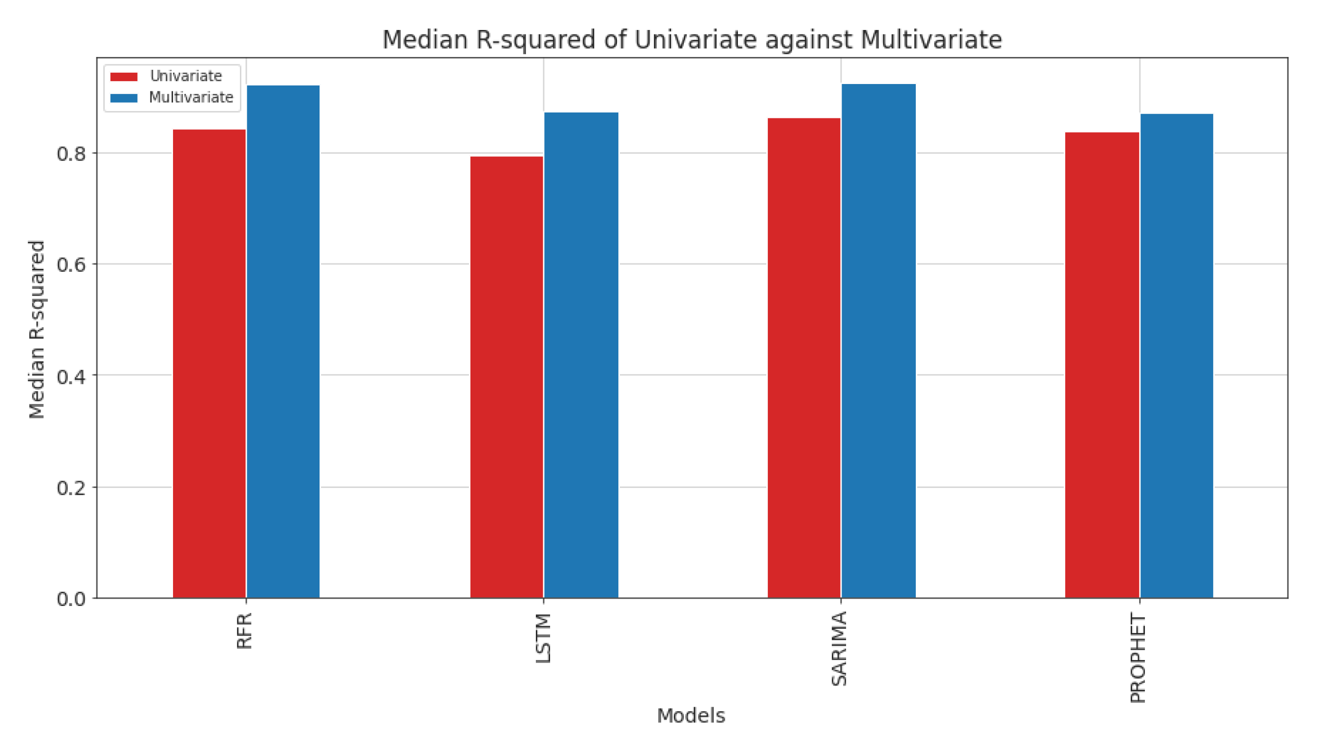
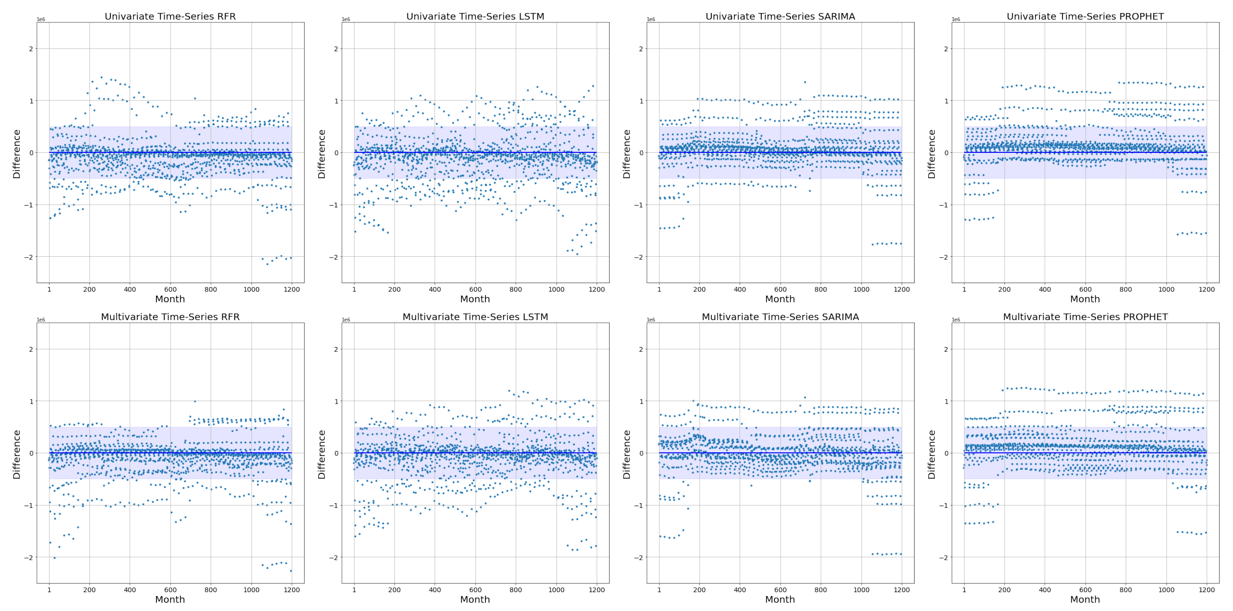
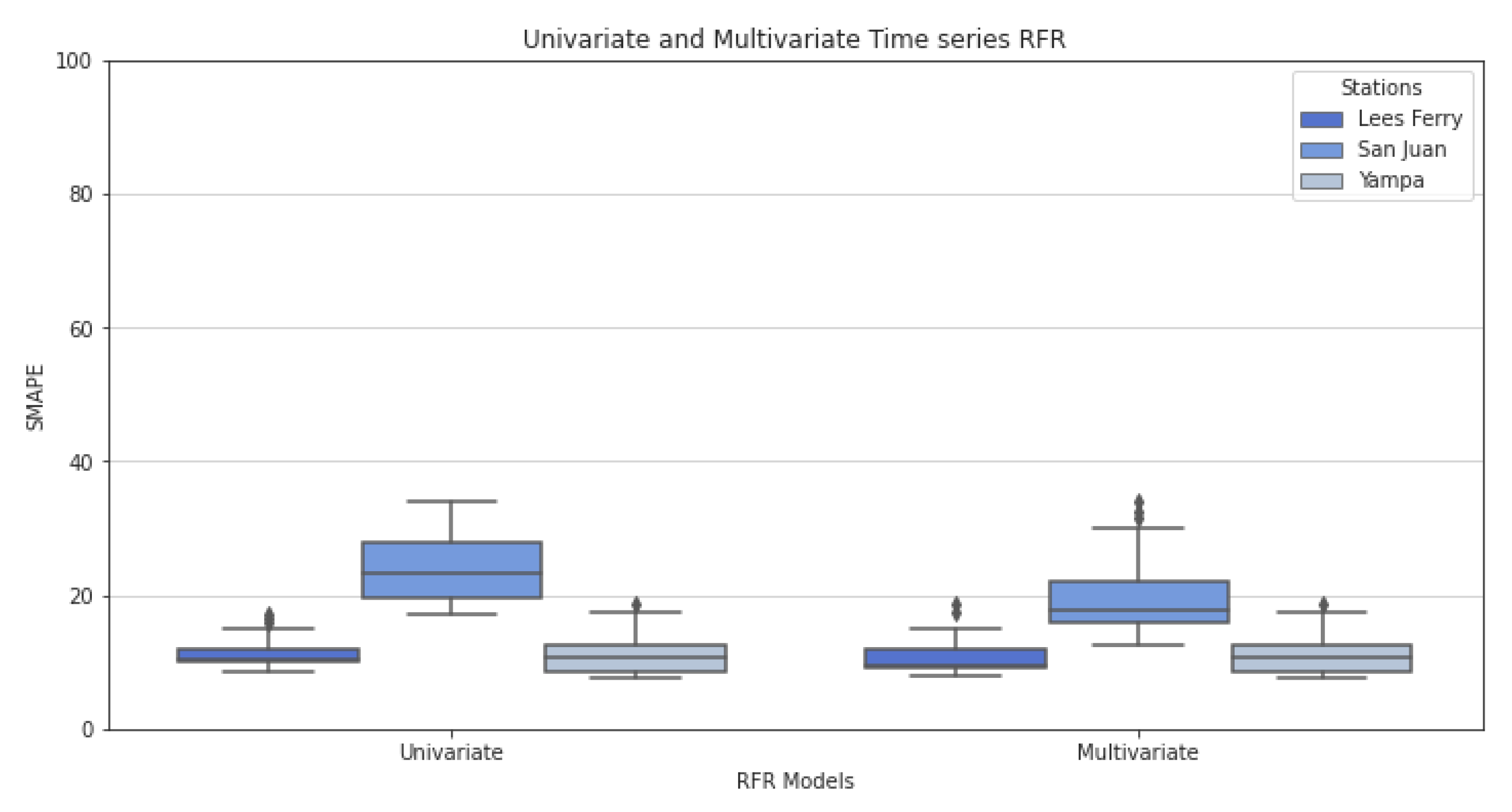
5.2. Univariate and Multivariate Time-Series Comparison
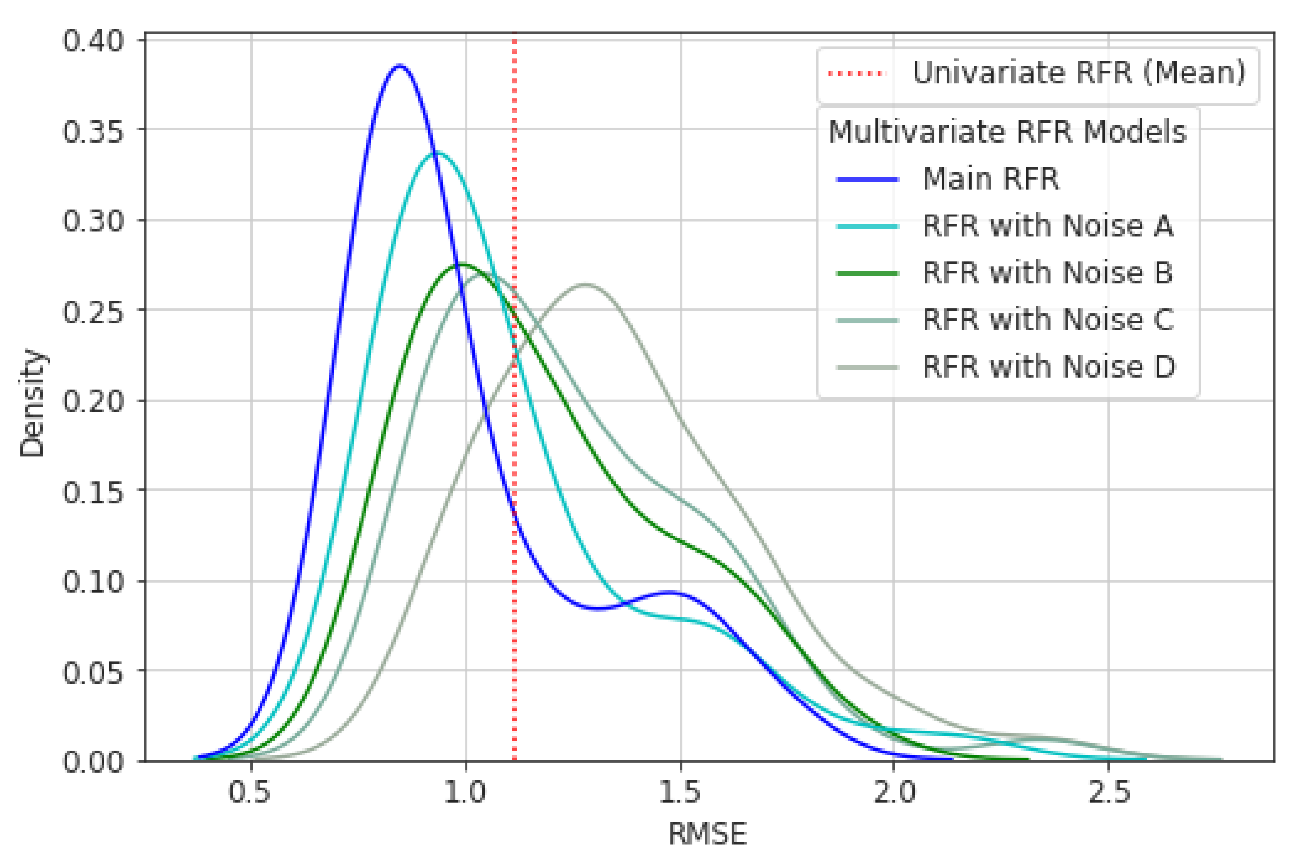
5.3. Sensitivity Analysis
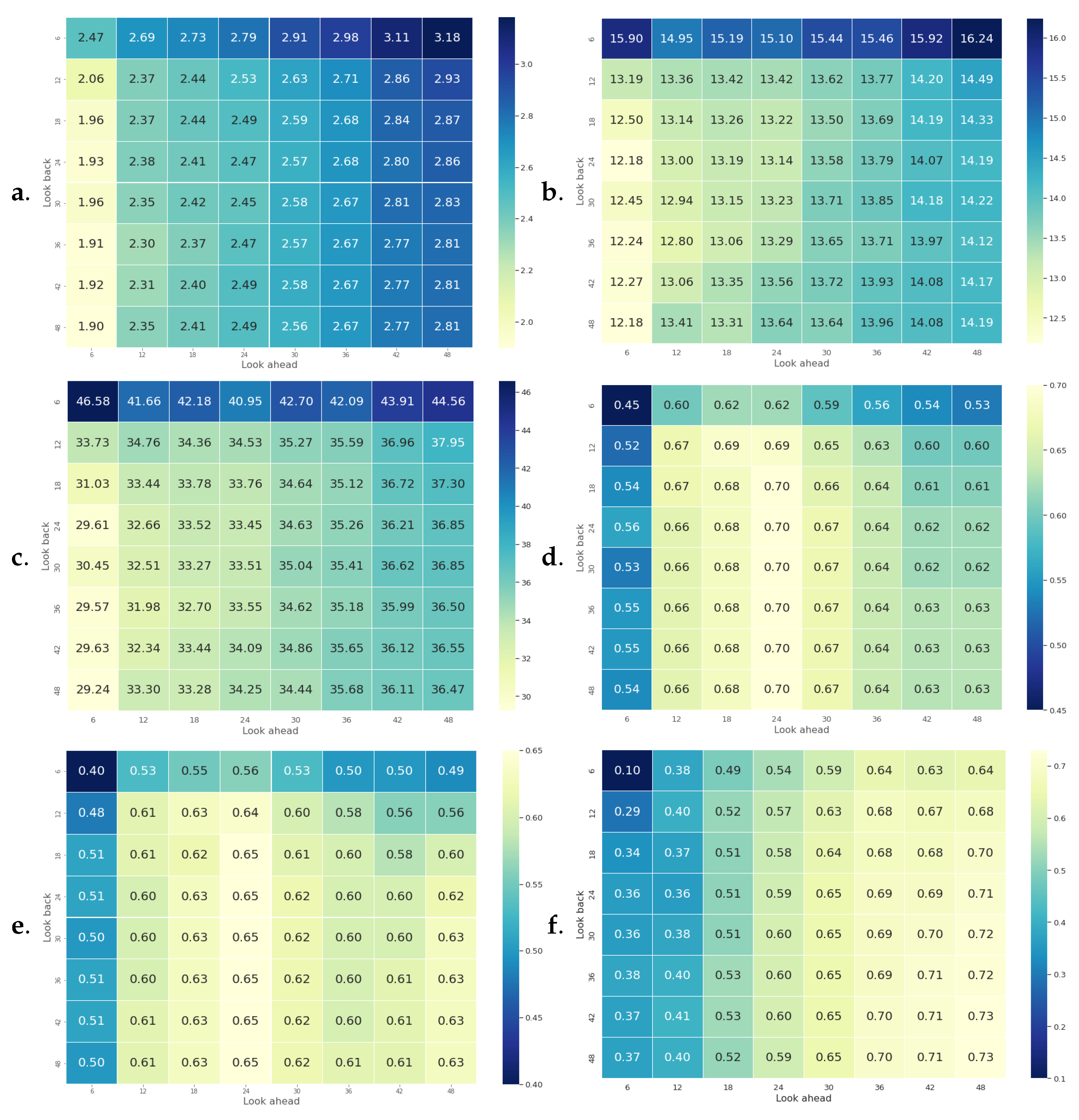
5.4. Sequence Analysis
6. Discussions
7. Conclusions
Author Contributions
Funding
Data Availability Statement
Conflicts of Interest
References
- Bai, J.; Shi, H.; Yu, Q.; Xie, Z.; Li, L.; Luo, G.; Jin, N.; Li, J. Satellite-observed vegetation stability in response to changes in climate and total water storage in Central Asia. Sci. Total Environ. 2019, 659, 862–871. [Google Scholar] [CrossRef]
- Sabzi, H.Z.; Moreno, H.A.; Fovargue, R.; Xue, X.; Hong, Y.; Neeson, T.M. Comparison of projected water availability and demand reveals future hotspots of water stress in the Red River basin, USA. J. Hydrol. Reg. Stud. 2019, 26, 100638. [Google Scholar] [CrossRef]
- Hannaford, J. Climate-driven changes in UK river flows: A review of the evidence. Prog. Phys. Geogr. 2015, 39, 29–48. [Google Scholar] [CrossRef] [Green Version]
- Milly, P.C.; Dunne, K.A.; Vecchia, A.V. Global pattern of trends in streamflow and water availability in a changing climate. Nature 2005, 438, 347–350. [Google Scholar] [CrossRef] [PubMed]
- Chen, H.; Xu, Y.P.; Teegavarapu, R.S.; Guo, Y.; Xie, J. Assessing different roles of baseflow and surface runoff for long-term streamflow forecasting in southeastern China. Hydrol. Sci. J. 2021, 66, 2312–2329. [Google Scholar] [CrossRef]
- Golembesky, K.; Sankarasubramanian, A.; Devineni, N. Improved drought management of Falls Lake Reservoir: Role of multimodel streamflow forecasts in setting up restrictions. J. Water Resour. Plan. Manag. 2009, 135, 188–197. [Google Scholar] [CrossRef]
- Lorenz, E.N. The predictability of a flow which possesses many scales of motion. Tellus 1969, 21, 289–307. [Google Scholar] [CrossRef]
- Delgado-Ramos, F.; Hervás-Gámez, C. Simple and low-cost procedure for monthly and yearly streamflow forecasts during the current hydrological year. Water 2018, 10, 1038. [Google Scholar] [CrossRef] [Green Version]
- Donegan, S.; Murphy, C.; Harrigan, S.; Broderick, C.; Foran Quinn, D.; Golian, S.; Knight, J.; Matthews, T.; Prudhomme, C.; Scaife, A.A.; et al. Conditioning ensemble streamflow prediction with the North Atlantic Oscillation improves skill at longer lead times. Hydrol. Earth Syst. Sci. 2021, 25, 4159–4183. [Google Scholar] [CrossRef]
- Arnal, L.; Cloke, H.L.; Stephens, E.; Wetterhall, F.; Prudhomme, C.; Neumann, J.; Krzeminski, B.; Pappenberger, F. Skilful seasonal forecasts of streamflow over Europe? Hydrol. Earth Syst. Sci. 2018, 22, 2057–2072. [Google Scholar] [CrossRef]
- Eldardiry, H.; Hossain, F. The value of long-term streamflow forecasts in adaptive reservoir operation: The case of the High Aswan Dam in the transboundary Nile River basin. J. Hydrometeorol. 2021, 22, 1099–1115. [Google Scholar] [CrossRef]
- Souza Filho, F.A.; Lall, U. Seasonal to interannual ensemble streamflow forecasts for Ceara, Brazil: Applications of a multivariate, semiparametric algorithm. Water Resour. Res. 2003, 39, 1307. [Google Scholar] [CrossRef]
- Liu, P.; Wang, L.; Ranjan, R.; He, G.; Zhao, L. A survey on active deep learning: From model-driven to data-driven. ACM Comput. Surv. 2021, 54, 1–34. [Google Scholar] [CrossRef]
- Brêda, J.P.L.F.; de Paiva, R.C.D.; Collischon, W.; Bravo, J.M.; Siqueira, V.A.; Steinke, E.B. Climate change impacts on South American water balance from a continental-scale hydrological model driven by CMIP5 projections. Clim. Chang. 2020, 159, 503–522. [Google Scholar] [CrossRef]
- Vieux, B.E.; Cui, Z.; Gaur, A. Evaluation of a physics-based distributed hydrologic model for flood forecasting. J. Hydrol. 2004, 298, 155–177. [Google Scholar] [CrossRef]
- Zang, S.; Li, Z.; Zhang, K.; Yao, C.; Liu, Z.; Wang, J.; Huang, Y.; Wang, S. Improving the flood prediction capability of the Xin’anjiang model by formulating a new physics-based routing framework and a key routing parameter estimation method. J. Hydrol. 2021, 603, 126867. [Google Scholar] [CrossRef]
- Lu, D.; Konapala, G.; Painter, S.L.; Kao, S.C.; Gangrade, S. Streamflow simulation in data-scarce basins using bayesian and physics-informed machine learning models. J. Hydrometeorol. 2021, 22, 1421–1438. [Google Scholar] [CrossRef]
- Clark, M.P.; Bierkens, M.F.; Samaniego, L.; Woods, R.A.; Uijlenhoet, R.; Bennett, K.E.; Pauwels, V.; Cai, X.; Wood, A.W.; Peters-Lidard, C.D. The evolution of process-based hydrologic models: Historical challenges and the collective quest for physical realism. Hydrol. Earth Syst. Sci. 2017, 21, 3427–3440. [Google Scholar] [CrossRef] [Green Version]
- Mei, X.; Van Gelder, P.; Dai, Z.; Tang, Z. Impact of dams on flood occurrence of selected rivers in the United States. Front. Earth Sci. 2017, 11, 268–282. [Google Scholar] [CrossRef]
- Riley, M.; Grandhi, R. A method for the quantification of model-form and parametric uncertainties in physics-based simulations. In Proceedings of the 52nd AIAA/ASME/ASCE/AHS/ASC Structures, Structural Dynamics and Materials Conference 19th AIAA/ASME/AHS Adaptive Structures Conference 13t, Denver, CO, USA, 4–7 April 2011; p. 1765. [Google Scholar]
- Siddiqi, T.A.; Ashraf, S.; Khan, S.A.; Iqbal, M.J. Estimation of data-driven streamflow predicting models using machine learning methods. Arab. J. Geosci. 2021, 14, 1–9. [Google Scholar] [CrossRef]
- Gauch, M.; Mai, J.; Gharari, S.; Lin, J. Data-driven vs. physically-based streamflow prediction models. In Proceedings of the 9th International Workshop on Climate Informatics, Paris, France, 2–4 October 2019. [Google Scholar]
- Mosavi, A.; Ozturk, P.; Chau, K.w. Flood prediction using machine learning models: Literature review. Water 2018, 10, 1536. [Google Scholar] [CrossRef] [Green Version]
- Gauch, M. Machine Learning for Streamflow Prediction. Master’s Thesis, University of Waterloo, Waterloo, ON, Canada, 2020. [Google Scholar]
- Rasouli, K. Short Lead-Time Streamflow Forecasting by Machine Learning Methods, with Climate Variability Incorporated. Ph.D. Thesis, University of British Columbia Vancouver, Vancouver, BC, Canada, 2010. [Google Scholar]
- Yan, J.; Jia, S.; Lv, A.; Zhu, W. Water resources assessment of China’s transboundary river basins using a machine learning approach. Water Resour. Res. 2019, 55, 632–655. [Google Scholar] [CrossRef] [Green Version]
- Gumiere, S.J.; Camporese, M.; Botto, A.; Lafond, J.A.; Paniconi, C.; Gallichand, J.; Rousseau, A.N. Machine learning vs. physics-based modeling for real-time irrigation management. Front. Water 2020, 2, 8. [Google Scholar] [CrossRef] [Green Version]
- Kumar, K.; Jain, V.K. Autoregressive integrated moving averages (ARIMA) modelling of a traffic noise time series. Appl. Acoust. 1999, 58, 283–294. [Google Scholar] [CrossRef]
- Valipour, M.; Banihabib, M.E.; Behbahani, S.M.R. Comparison of the ARMA, ARIMA, and the autoregressive artificial neural network models in forecasting the monthly inflow of Dez dam reservoir. J. Hydrol. 2013, 476, 433–441. [Google Scholar] [CrossRef]
- Ghimire, B.N. Application of ARIMA model for river discharges analysis. J. Nepal Phys. Soc. 2017, 4, 27–32. [Google Scholar] [CrossRef] [Green Version]
- Valipour, M. Long-term runoff study using SARIMA and ARIMA models in the United States. Meteorol. Appl. 2015, 22, 592–598. [Google Scholar] [CrossRef]
- Taylor, S.J.; Letham, B. Forecasting at scale. Am. Stat. 2018, 72, 37–45. [Google Scholar] [CrossRef]
- Basak, A.; Rahman, A.S.; Das, J.; Hosono, T.; Kisi, O. Drought forecasting using the Prophet model in a semi-arid climate region of western India. Hydrol. Sci. J. 2022, 67, 1397–1417. [Google Scholar] [CrossRef]
- Rahman, A.S.; Hosono, T.; Kisi, O.; Dennis, B.; Imon, A.R. A minimalistic approach for evapotranspiration estimation using the Prophet model. Hydrol. Sci. J. 2020, 65, 1994–2006. [Google Scholar] [CrossRef]
- Xiao, Q.; Zhou, L.; Xiang, X.; Liu, L.; Liu, X.; Li, X.; Ao, T. Integration of Hydrological Model and Time Series Model for Improving the Runoff Simulation: A Case Study on BTOP Model in Zhou River Basin, China. Appl. Sci. 2022, 12, 6883. [Google Scholar] [CrossRef]
- Segal, M.R. Machine Learning Benchmarks and Random Forest Regression; Kluwer Academic Publishers: Dordrecht, The Netherlands, 2004. [Google Scholar]
- Zhang, Y.; Chiew, F.H.; Li, M.; Post, D. Predicting runoff signatures using regression and hydrological modeling approaches. Water Resour. Res. 2018, 54, 7859–7878. [Google Scholar] [CrossRef]
- Li, J.; Wang, Z.; Lai, C.; Zhang, Z. Tree-ring-width based streamflow reconstruction based on the random forest algorithm for the source region of the Yangtze River, China. Catena 2019, 183, 104216. [Google Scholar] [CrossRef]
- Kombo, O.H.; Kumaran, S.; Sheikh, Y.H.; Bovim, A.; Jayavel, K. Long-term groundwater level prediction model based on hybrid KNN-RF technique. Hydrology 2020, 7, 59. [Google Scholar] [CrossRef]
- Dastjerdi, S.Z.; Sharifi, E.; Rahbar, R.; Saghafian, B. Downscaling WGHM-Based Groundwater Storage Using Random Forest Method: A Regional Study over Qazvin Plain, Iran. Hydrology 2022, 9, 179. [Google Scholar] [CrossRef]
- Yu, Y.; Si, X.; Hu, C.; Zhang, J. A review of recurrent neural networks: LSTM cells and network architectures. Neural Comput. 2019, 31, 1235–1270. [Google Scholar] [CrossRef]
- Hu, Y.; Yan, L.; Hang, T.; Feng, J. Stream-flow forecasting of small rivers based on LSTM. arXiv 2020, arXiv:2001.05681. [Google Scholar]
- Fu, M.; Fan, T.; Ding, Z.; Salih, S.Q.; Al-Ansari, N.; Yaseen, Z.M. Deep learning data-intelligence model based on adjusted forecasting window scale: Application in daily streamflow simulation. IEEE Access 2020, 8, 32632–32651. [Google Scholar] [CrossRef]
- Kratzert, F.; Klotz, D.; Brenner, C.; Schulz, K.; Herrnegger, M. Rainfall–runoff modelling using long short-term memory (LSTM) networks. Hydrol. Earth Syst. Sci. 2018, 22, 6005–6022. [Google Scholar] [CrossRef] [Green Version]
- Rahimzad, M.; Moghaddam Nia, A.; Zolfonoon, H.; Soltani, J.; Danandeh Mehr, A.; Kwon, H.H. Performance comparison of an lstm-based deep learning model versus conventional machine learning algorithms for streamflow forecasting. Water Resour. Manag. 2021, 35, 4167–4187. [Google Scholar] [CrossRef]
- Alizadeh, B.; Bafti, A.G.; Kamangir, H.; Zhang, Y.; Wright, D.B.; Franz, K.J. A novel attention-based LSTM cell post-processor coupled with bayesian optimization for streamflow prediction. J. Hydrol. 2021, 601, 126526. [Google Scholar] [CrossRef]
- Feng, D.; Fang, K.; Shen, C. Enhancing streamflow forecast and extracting insights using long-short term memory networks with data integration at continental scales. Water Resour. Res. 2020, 56, e2019WR026793. [Google Scholar] [CrossRef]
- Apaydin, H.; Sattari, M.T.; Falsafian, K.; Prasad, R. Artificial intelligence modelling integrated with Singular Spectral analysis and Seasonal-Trend decomposition using Loess approaches for streamflow predictions. J. Hydrol. 2021, 600, 126506. [Google Scholar] [CrossRef]
- Ghimire, S.; Yaseen, Z.M.; Farooque, A.A.; Deo, R.C.; Zhang, J.; Tao, X. Streamflow prediction using an integrated methodology based on convolutional neural network and long short-term memory networks. Sci. Rep. 2021, 11, 1–26. [Google Scholar] [CrossRef]
- Le, X.H.; Nguyen, D.H.; Jung, S.; Yeon, M.; Lee, G. Comparison of deep learning techniques for river streamflow forecasting. IEEE Access 2021, 9, 71805–71820. [Google Scholar] [CrossRef]
- Risbey, J.S.; Entekhabi, D. Observed Sacramento Basin streamflow response to precipitation and temperature changes and its relevance to climate impact studies. J. Hydrol. 1996, 184, 209–223. [Google Scholar] [CrossRef]
- Fu, G.; Charles, S.P.; Chiew, F.H. A two-parameter climate elasticity of streamflow index to assess climate change effects on annual streamflow. Water Resour. Res. 2007, 43, W11419. [Google Scholar] [CrossRef]
- Xu, T.; Longyang, Q.; Tyson, C.; Zeng, R.; Neilson, B.T. Hybrid Physically Based and Deep Learning Modeling of a Snow Dominated, Mountainous, Karst Watershed. Water Resour. Res. 2022, 58, e2021WR030993. [Google Scholar] [CrossRef]
- Asefa, T.; Kemblowski, M.; McKee, M.; Khalil, A. Multi-time scale stream flow predictions: The support vector machines approach. J. Hydrol. 2006, 318, 7–16. [Google Scholar] [CrossRef]
- Zhao, S.; Fu, R.; Zhuang, Y.; Wang, G. Long-lead seasonal prediction of streamflow over the Upper Colorado River Basin: The role of the Pacific sea surface temperature and beyond. J. Clim. 2021, 34, 6855–6873. [Google Scholar] [CrossRef]
- Water, G. The Sustainable Use of Water in the Lower Colorado River Basin; Pacific Institute for Studies in Development, Environment, and Security: Oakland, CA, USA, 1996. [Google Scholar]
- Vano, J.A.; Udall, B.; Cayan, D.R.; Overpeck, J.T.; Brekke, L.D.; Das, T.; Hartmann, H.C.; Hidalgo, H.G.; Hoerling, M.; McCabe, G.J.; et al. Understanding uncertainties in future Colorado River streamflow. Bull. Am. Meteorol. Soc. 2014, 95, 59–78. [Google Scholar] [CrossRef]
- Smith, J.A.; Baeck, M.L.; Yang, L.; Signell, J.; Morin, E.; Goodrich, D.C. The paroxysmal precipitation of the desert: Flash floods in the Southwestern United States. Water Resour. Res. 2019, 55, 10218–10247. [Google Scholar] [CrossRef]
- Barnett, T.P.; Pierce, D.W. Sustainable water deliveries from the Colorado River in a changing climate. Proc. Natl. Acad. Sci. USA 2009, 106, 7334–7338. [Google Scholar] [CrossRef] [PubMed] [Green Version]
- Cohen, M.; Christian-Smith, J.; Berggren, J. Water to supply the land. Pac. Inst. 2013. [Google Scholar]
- Xiao, M.; Udall, B.; Lettenmaier, D.P. On the causes of declining Colorado River streamflows. Water Resour. Res. 2018, 54, 6739–6756. [Google Scholar] [CrossRef]
- Board, C.W.C. Flood Hazard Mitigation Plan for Colorado. Integration 2010, 2, 1. [Google Scholar]
- Kopytkovskiy, M.; Geza, M.; McCray, J. Climate-change impacts on water resources and hydropower potential in the Upper Colorado River Basin. J. Hydrol. Reg. Stud. 2015, 3, 473–493. [Google Scholar] [CrossRef] [Green Version]
- Rumsey, C.A.; Miller, M.P.; Schwarz, G.E.; Hirsch, R.M.; Susong, D.D. The role of baseflow in dissolved solids delivery to streams in the Upper Colorado River Basin. Hydrol. Process. 2017, 31, 4705–4718. [Google Scholar] [CrossRef]
- Hadjimichael, A.; Quinn, J.; Wilson, E.; Reed, P.; Basdekas, L.; Yates, D.; Garrison, M. Defining robustness, vulnerabilities, and consequential scenarios for diverse stakeholder interests in institutionally complex river basins. Earth’s Future 2020, 8, e2020EF001503. [Google Scholar] [CrossRef]
- Hwang, J.; Kumar, H.; Ruhi, A.; Sankarasubramanian, A.; Devineni, N. Quantifying Dam-Induced Fluctuations in Streamflow Frequencies Across the Colorado River Basin. Water Resour. Res. 2021, 57, e2021WR029753. [Google Scholar] [CrossRef]
- Kirk, J.P.; Schmidlin, T.W. Moisture transport associated with large precipitation events in the Upper Colorado River Basin. Int. J. Climatol. 2018, 38, 5323–5338. [Google Scholar] [CrossRef]
- Ayers, J.; Ficklin, D.L.; Stewart, I.T.; Strunk, M. Comparison of CMIP3 and CMIP5 projected hydrologic conditions over the Upper Colorado River Basin. Int. J. Climatol. 2016, 36, 3807–3818. [Google Scholar] [CrossRef] [Green Version]
- Salehabadi, H.; Tarboton, D.; Kuhn, E.; Udall, B.; Wheeler, K.; Rosenberg, D.; Goeking, S.; Schmidt, J.C. The future hydrology of the Colorado River Basin. In The Future of the Colorado River Project; White Paper No. 4; Utah State University, Quinney College of Natural Resources Center for Colorado River Studies: Logan, UT, USA, 2020; 71p. [Google Scholar]
- Lukas, J.; Payton, E. Colorado River Basin Climate and Hydrology: State of the Science; Western Water Assessment, University of Colorado Boulder: Boulder, CO, USA, 2020. [Google Scholar]
- McCabe, G.J.; Wolock, D.M.; Pederson, G.T.; Woodhouse, C.A.; McAfee, S. Evidence that recent warming is reducing upper Colorado River flows. Earth Interact. 2017, 21, 1–14. [Google Scholar] [CrossRef]
- McCoy, A.L.; Jacobs, K.L.; Vano, J.A.; Wilson, J.K.; Martin, S.; Pendergrass, A.G.; Cifelli, R. The Press and Pulse of Climate Change: Extreme Events in the Colorado River Basin. JAWRA J. Am. Water Resour. Assoc. 2022, 58, 1076–1097. [Google Scholar] [CrossRef]
- Kappal, S. Data normalization using median median absolute deviation MMAD based Z-score for robust predictions vs. min–max normalization. Lond. J. Res. Sci. Nat. Form. 2019, 19. [Google Scholar]
- Toharudin, T.; Pontoh, R.S.; Caraka, R.E.; Zahroh, S.; Lee, Y.; Chen, R.C. Employing long short-term memory and Facebook prophet model in air temperature forecasting. Commun.-Stat.-Simul. Comput. 2020, 52, 279–290. [Google Scholar] [CrossRef]
- Bercu, S.; Proïa, F. A SARIMAX coupled modelling applied to individual load curves intraday forecasting. J. Appl. Stat. 2013, 40, 1333–1348. [Google Scholar] [CrossRef] [Green Version]
- Sarhadi, A.; Kelly, R.; Modarres, R. Snow water equivalent time-series forecasting in Ontario, Canada, in link to large atmospheric circulations. Hydrol. Process. 2014, 28, 4640–4653. [Google Scholar] [CrossRef]
- Kim, S.; Kim, H. A new metric of absolute percentage error for intermittent demand forecasts. Int. J. Forecast. 2016, 32, 669–679. [Google Scholar] [CrossRef]
- Nash, J.E.; Sutcliffe, J.V. River flow forecasting through conceptual models part I—A discussion of principles. J. Hydrol. 1970, 10, 282–290. [Google Scholar] [CrossRef]
- Gupta, H.V.; Kling, H.; Yilmaz, K.K.; Martinez, G.F. Decomposition of the mean squared error and NSE performance criteria: Implications for improving hydrological modelling. J. Hydrol. 2009, 377, 80–91. [Google Scholar] [CrossRef] [Green Version]
- Shortridge, J.E.; Guikema, S.D.; Zaitchik, B.F. Machine learning methods for empirical streamflow simulation: A comparison of model accuracy, interpretability, and uncertainty in seasonal watersheds. Hydrol. Earth Syst. Sci. 2016, 20, 2611–2628. [Google Scholar] [CrossRef] [Green Version]
- Al-Mukhtar, M. Random forest, support vector machine, and neural networks to modelling suspended sediment in Tigris River-Baghdad. Environ. Monit. Assess. 2019, 191, 1–12. [Google Scholar] [CrossRef] [PubMed]
- Minns, A.; Hall, M. Artificial neural networks as rainfall-runoff models. Hydrol. Sci. J. 1996, 41, 399–417. [Google Scholar] [CrossRef]
- Francke, T.; López-Tarazón, J.; Schröder, B. Estimation of suspended sediment concentration and yield using linear models, random forests and quantile regression forests. Hydrol. Process. Int. J. 2008, 22, 4892–4904. [Google Scholar] [CrossRef]
- Aguilera, H.; Guardiola-Albert, C.; Naranjo-Fernández, N.; Kohfahl, C. Towards flexible groundwater-level prediction for adaptive water management: Using Facebook’s Prophet forecasting approach. Hydrol. Sci. J. 2019, 64, 1504–1518. [Google Scholar] [CrossRef]
- Khodakhah, H.; Aghelpour, P.; Hamedi, Z. Comparing linear and non-linear data-driven approaches in monthly river flow prediction, based on the models SARIMA, LSSVM, ANFIS, and GMDH. Environ. Sci. Pollut. Res. 2022, 29, 21935–21954. [Google Scholar] [CrossRef]
- Yaghoubi, B.; Hosseini, S.A.; Nazif, S. Monthly prediction of streamflow using data-driven models. J. Earth Syst. Sci. 2019, 128, 1–15. [Google Scholar] [CrossRef] [Green Version]
- Livieris, I.E.; Pintelas, E.; Pintelas, P. A CNN–LSTM model for gold price time-series forecasting. Neural Comput. Appl. 2020, 32, 17351–17360. [Google Scholar] [CrossRef]
- Lu, W.; Li, J.; Li, Y.; Sun, A.; Wang, J. A CNN-LSTM-based model to forecast stock prices. Complexity 2020, 2020, 6622927. [Google Scholar] [CrossRef]
- Vaswani, A.; Shazeer, N.; Parmar, N.; Uszkoreit, J.; Jones, L.; Gomez, A.N.; Kaiser, Ł; Polosukhin, I. Attention is all you need. Adv. Neural Inf. Process. Syst. 2017, 30. [Google Scholar]
- Wang, C.; Chen, Y.; Zhang, S.; Zhang, Q. Stock market index prediction using deep Transformer model. Expert Syst. Appl. 2022, 208, 118128. [Google Scholar] [CrossRef]


| Univariate Time-Series | Multivariate Time-Series | ||||
|---|---|---|---|---|---|
| ID | Model | Count | Percent (%) | Count | Percent (%) |
| 1 | RFR | 976 | 81 | 1001 | 83 |
| 2 | LSTM | 894 | 74 | 950 | 79 |
| 3 | SARIMA | 991 | 82 | 1054 | 87 |
| 4 | PROPHET | 990 | 82 | 998 | 82 |
Disclaimer/Publisher’s Note: The statements, opinions and data contained in all publications are solely those of the individual author(s) and contributor(s) and not of MDPI and/or the editor(s). MDPI and/or the editor(s) disclaim responsibility for any injury to people or property resulting from any ideas, methods, instructions or products referred to in the content. |
© 2023 by the authors. Licensee MDPI, Basel, Switzerland. This article is an open access article distributed under the terms and conditions of the Creative Commons Attribution (CC BY) license (https://creativecommons.org/licenses/by/4.0/).
Share and Cite
Hosseinzadeh, P.; Nassar, A.; Boubrahimi, S.F.; Hamdi, S.M. ML-Based Streamflow Prediction in the Upper Colorado River Basin Using Climate Variables Time Series Data. Hydrology 2023, 10, 29. https://doi.org/10.3390/hydrology10020029
Hosseinzadeh P, Nassar A, Boubrahimi SF, Hamdi SM. ML-Based Streamflow Prediction in the Upper Colorado River Basin Using Climate Variables Time Series Data. Hydrology. 2023; 10(2):29. https://doi.org/10.3390/hydrology10020029
Chicago/Turabian StyleHosseinzadeh, Pouya, Ayman Nassar, Soukaina Filali Boubrahimi, and Shah Muhammad Hamdi. 2023. "ML-Based Streamflow Prediction in the Upper Colorado River Basin Using Climate Variables Time Series Data" Hydrology 10, no. 2: 29. https://doi.org/10.3390/hydrology10020029