
Estimating Thermal Impact on Groundwater Systems from Heat Pump Technologies: A Simplified Method for High Flow Rates

Abstract
:1. Introduction
2. Materials and Methods
2.1. Hydraulics of a Two-Well Heat Pump System
2.1.1. Characteristics of the Heat Pump System
2.1.2. Determining the Backflow to the Pumping Well
2.2. Thermal Impact on Surroundings
- The radial transport model;
- The linear advective model of heat transport;
- The planar advective model of heat transport.
3. Results
3.1. Empirical Methods
3.1.1. Cloud Length
3.1.2. Cloud Width
3.1.3. Simplified Methodology for the Assessment of Heat Pump Technology
- The evaluation of the hydraulic separation of the wells. If the wells are hydraulically separated, there is no increase in temperature in the pumped well due to the inflow of already heated water. If the condition from Equation (4) is met, the wells are hydraulically separated, and one can advance to step 3. If not, progression to step 2 is required.
- The determination of the time of temperature backflow. If the wells are not hydraulically separated, the resulting system can still be used until the thermally adjusted water flows back into the pumped well. From the Equation (9), the water flow duration () is calculated, and subsequently, the heat transport time () is derived from Equation (11). If the heat transport time is less than the number of days in the heating/cooling seasons, the wells thermally influence each other.
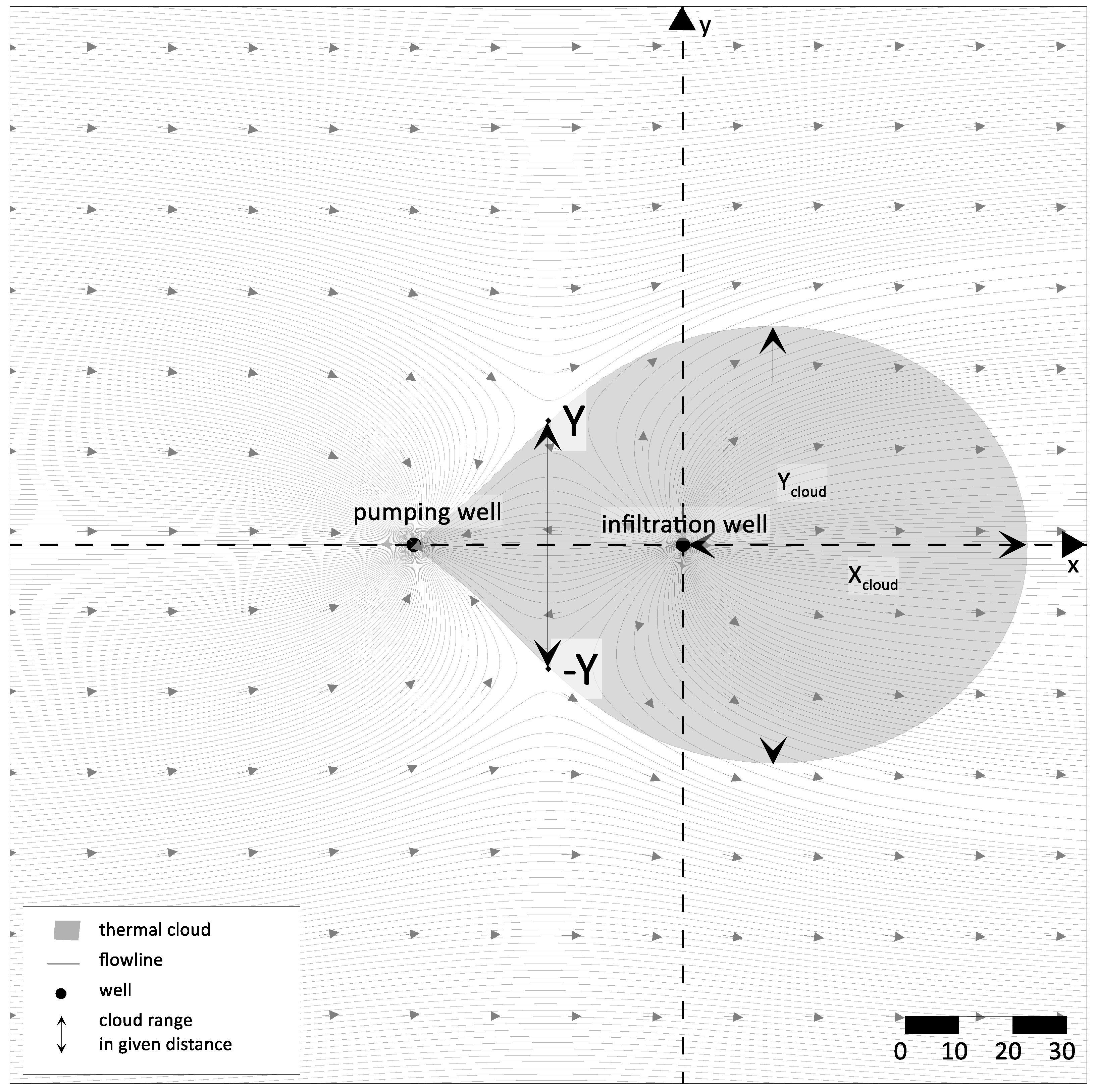
- The estimation of the thermal cloud’s extent. This involves determining the estimated dimensions of the thermal cloud that will spread into the surroundings according to Figure 3. The length of the cloud () is calculated from Equation (22), and the width of the cloud () is calculated from Equation (23). It should be noted that the dimensions of the thermal cloud are ascertained based on the numerical modeling of an idealized scenario. These should be overestimated values, determined at a thermal gradient of 12 °C. The boundaries are selected lines at which the thermal change compared to the original state is 1 °C. If the gradient of the poured water is smaller, we cannot predict how the boundaries will diminish or expand, only that the temperature change on the given line will be directly proportionally smaller. Such calculated values are never superior to more precise calculations as this is a very rough approximation.
4. Discussion and Conclusions
Supplementary Materials
Author Contributions
Funding
Data Availability Statement
Conflicts of Interest
References
- Ampofo, F.; Maidment, G.; Missenden, J. Review of groundwater cooling systems in London. Appl. Therm. Eng. 2006, 26, 2055–2062. [Google Scholar] [CrossRef]
- Andersson, O. Heat pump supported ATES applications in Sweden. IEA Heat Pump Cent. Newsl. 1998, 16, 20–21. [Google Scholar]
- Bakema, G.; Snijders, A. ATES and ground-source heat pumps in the Netherlands. IEA Heat Pump Cent. Newsl. 1998, 16, 15–17. [Google Scholar]
- Ball, D.A.; Fischer, R.D.; Talbert, S.G.; Hodgett, D.; Auer, F. State of-the-Art Survey of Existing Knowledge for the Design of Ground Source Heat Pump Systems; Report ORNL/Sub 80-7800/2; Battelle Columbus Laboratories: Columbus, OH, USA, 1983; 75p. [Google Scholar]
- Banks, D. Thermogeological Assessment of Open-Loop Well-Doublet Schemes: A Review and Synthesis of Analytical Approaches. Hydrogeol. J. 2009, 17, 1149–1155. [Google Scholar] [CrossRef]
- Bodvarsson, G. Thermal problems in the siting of reinjection wells. Geothermics 1972, 1, 63–66. [Google Scholar] [CrossRef]
- Clyde, C.G.; Madabhushi, G.V. Spacing of wells for heat pumps. J. Water Resour. Plan. Manag. 1983, 109, 203–212. [Google Scholar] [CrossRef]
- De Marsily, G. Quantitative Hydrogeology: Groundwater Hydrology for Engineers; Academic: Orlando, FL, USA, 1986; pp. 277–283. [Google Scholar]
- Domenico, P.A.; Schwartz, F.W. Physical and Chemical Hydrogeology; Wiley: New York, NY, USA, 1990; 824p. [Google Scholar]
- Clauser, C. Numerical Simulation of Reactive Flow in Hot Aquifers: SHEMAT and Processing SHEMAT; Springer: Berlin/Heidelberg, Germany, 2003; 332p. [Google Scholar]
- Ferguson, G.; Woodbury, A.D. Thermal sustainability of groundwater-source cooling in Winnipeg, Manitoba. Can. Geotech. J. 2005, 42, 1290–1301. [Google Scholar] [CrossRef]
- Gringarten, A.C. Reservoir lifetime and heat recovery factor in geothermal aquifers used for urban heating. Pure Appl. Geophys. 1978, 117, 297–308. [Google Scholar] [CrossRef]
- Liu, G.; Pu, H.; Zhao, Z.; Liu, Y. Coupled thermo-hydro-mechanical modeling on well pairs in heterogeneous porous geothermal reservoirs. Energy 2019, 171, 631–653. [Google Scholar] [CrossRef]
- Di Dato, M.; D’angelo, C.; Casasso, A.; Zarlenga, A. The impact of porous medium heterogeneity on the thermal feedback of open-loop shallow geothermal systems. J. Hydrol. 2022, 604, 127205. [Google Scholar] [CrossRef]
- Gringarten, A.C.; Sauty, J.P. A theoretical study of heat extraction from aquifers with uniform regional flow. J. Geophys. Res. 1975, 80, 4956–4962. [Google Scholar] [CrossRef]
- Tsang, C.F.; Lippmann, M.J.; Witherspoon, P.A. Production and reinjection in geothermal reservoirs. Trans. Geotherm. Resour. Counc. 1977, 1, 301–303. [Google Scholar]
- Pophillat, W.; Attard, G.; Bayer, P.; Hecht-Méndez, J.; Blum, P. Analytical solutions for predicting thermal plumes of groundwater heat pump systems. Renew. Energy 2020, 147, 2696–2707. [Google Scholar] [CrossRef]
- Banks, D. An Introduction to Thermogeology: Ground Source Heating and Cooling, 2nd ed.; Wiley: Chichester, UK, 2012; 544p. [Google Scholar]
- Luo, J.; Kitanidis, P.K. Fluid residence times within a recirculation zone created by an extraction–injection well pair. J. Hydrol. 2004, 295, 149–162. [Google Scholar] [CrossRef]
- Milnes, E.; Perrochet, P. Assessing the impact of thermal feedback and recycling in open-loop groundwater heat pump (GWHP) systems: A complementary design tool. Hydrogeol. J. 2013, 21, 505–514. [Google Scholar] [CrossRef]
- Piga, B.; Casasso, A.; Pace, F.; Godio, A.; Sethi, R. Thermal Impact Assessment of Groundwater Heat Pumps (GWHPs): Rigorous vs. Simplified Models. Energies 2017, 10, 1385. [Google Scholar] [CrossRef]
- McDonald, M.G.; Harbaugh, A.W. A Modular Three-Dimensional Finite-Difference Ground-Water Flow Model; Holcomb University: Indianapolis, IN, USA, 1988. [Google Scholar] [CrossRef]
- Zheng, C.; Wang, P.P. MT3DMS: A Modular 3-D Multispecies Model for Simulation of Advection, Dispersion and Chemical Reactions of Contaminants in Groundwater Systems. Documentation and User’s Guide; Contract Report SERDP-99-1; Army Engineer Research and Development Center: Vicksburg, MS, USA, 1999. [Google Scholar]
- Hetch-Mendéz, J. Implementation and Verification of the USGS Solute Transport Code MT3DMS for Groundwater Heat Transport Modeling. Master’s Thesis, University of Tübingen, Tübingen, Germany, 2008. [Google Scholar]


| Variable | Symbol | Unit |
|---|---|---|
| Temperature gradient of poured water | ΔTinj | K |
| Temperature gradient in the source term | ΔT0 | K |
| Width of the source term | Y | m |
| Poured amount of water | Q | m3/s |
| Seepage velocity | va | m/s |
| Specific heat capacity of substance x (w—water; s—solid) | cx | J/(kg·K) |
| Volumetric heat capacity of substance x (w—water; s—solid) | Cx | J/(m3·K) |
| Density of substance x (w—water; s—solid substance) | ρx | kg/m3 |
| Thermal conductivity of substance x (w—water; s—solid) | λx | W/(m·K) |
| Dispersion (transverse longitudinal) | αT,L | m |
| Retardation coefficient | R | --- |
| Parameter | Unit | Value |
|---|---|---|
| Water density | kg/m3 | 1000 |
| Specific heat capacity of water | J/(kg·K) | 4180 |
| Rock density—quartz | kg/m3 | 2600 |
| Specific heat capacity—quartz | J/(kg·K) | 820 |
| Thermal conductivity of porous environment | W/(m·K) | 2.5 |
| Longitudinal dispersion | m | 1.8 |
| Transverse dispersion | m | 0.18 |
| Parameter | Unit | Value Range |
|---|---|---|
| Thickness of aquifer | m | 4–20 |
| Pumped amount of water | L/s | 0–10 |
| Distance of wells | m | 30–100 |
| Groundwater gradient | m/m | 0.0005–0.002 |
| Hydraulic conductivity | m/s | 1 × 10⁻³–5 × 10⁻³ |
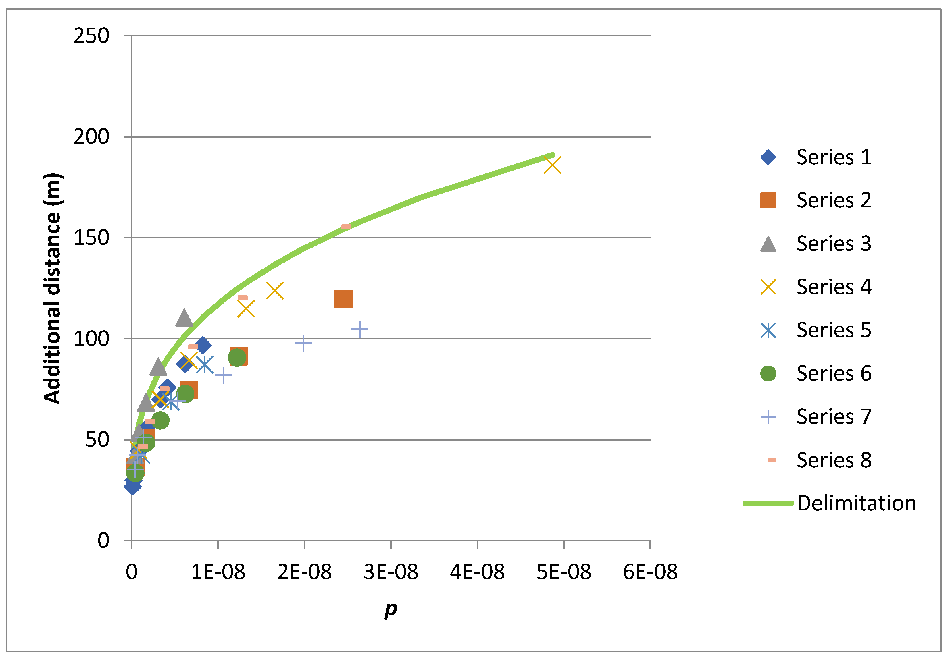
| Parameter | k | b | n | L | I |
|---|---|---|---|---|---|
| Unit | m/s | m | m | m/m | |
| Series 1 | 0.00125 | 10 | 0.3 | 50 | 0.001 |
| Series 2 | 0.00125 | 10 | 0.3 | 50 | 0.002 |
| Series 3 | 0.00125 | 10 | 0.3 | 50 | 0.0005 |
| Series 4 | 0.00125 | 2.5 | 0.3 | 50 | 0.001 |
| Series 5 | 0.00125 | 10 | 0.22 | 50 | 0.001 |
| Series 6 | 0.00125 | 10 | 0.3 | 20 | 0.001 |
| Series 7 | 0.004 | 10 | 0.3 | 50 | 0.001 |
| Series 8 | 0.001 | 4 | 0.3 | 50 | 0.001 |
Disclaimer/Publisher’s Note: The statements, opinions and data contained in all publications are solely those of the individual author(s) and contributor(s) and not of MDPI and/or the editor(s). MDPI and/or the editor(s) disclaim responsibility for any injury to people or property resulting from any ideas, methods, instructions or products referred to in the content. |
© 2023 by the authors. Licensee MDPI, Basel, Switzerland. This article is an open access article distributed under the terms and conditions of the Creative Commons Attribution (CC BY) license (https://creativecommons.org/licenses/by/4.0/).
Share and Cite
Krcmar, D.; Kovacs, T.; Molnar, M.; Hodasova, K.; Zatlakovic, M. Estimating Thermal Impact on Groundwater Systems from Heat Pump Technologies: A Simplified Method for High Flow Rates. Hydrology 2023, 10, 225. https://doi.org/10.3390/hydrology10120225
Krcmar D, Kovacs T, Molnar M, Hodasova K, Zatlakovic M. Estimating Thermal Impact on Groundwater Systems from Heat Pump Technologies: A Simplified Method for High Flow Rates. Hydrology. 2023; 10(12):225. https://doi.org/10.3390/hydrology10120225
Chicago/Turabian StyleKrcmar, David, Tibor Kovacs, Matej Molnar, Kamila Hodasova, and Martin Zatlakovic. 2023. "Estimating Thermal Impact on Groundwater Systems from Heat Pump Technologies: A Simplified Method for High Flow Rates" Hydrology 10, no. 12: 225. https://doi.org/10.3390/hydrology10120225