
Assessment of Potential Potable Water Reserves in Islamabad, Pakistan Using Vertical Electrical Sounding Technique
 ,
,  and
and
Abstract
:1. Introduction
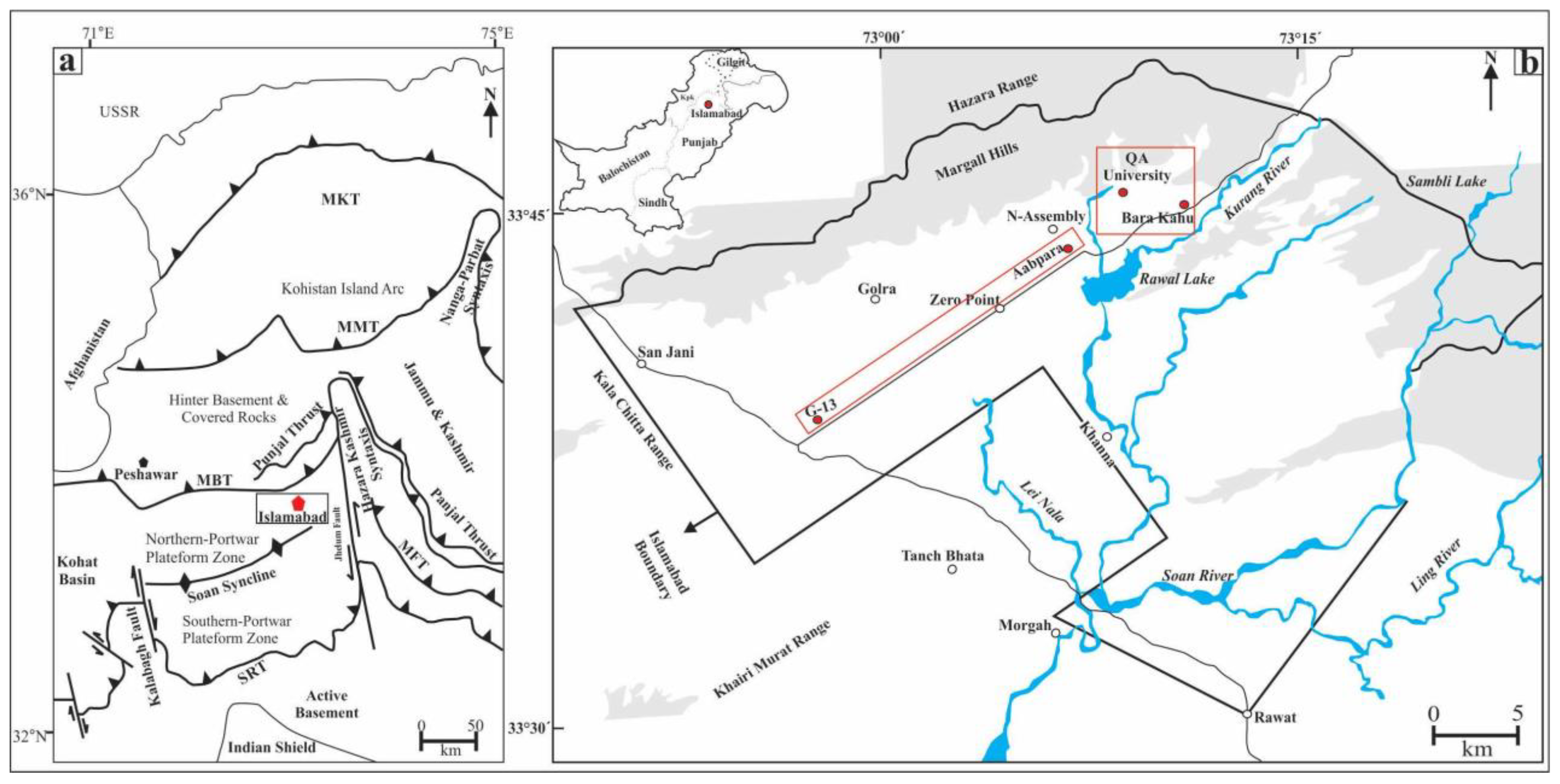
2. Study Area
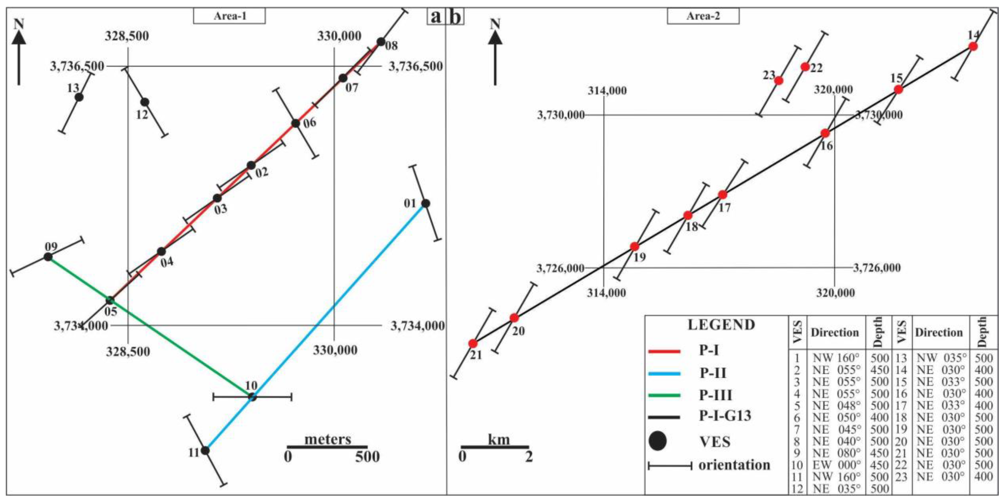
3. Methodology
4. Results and Discussion
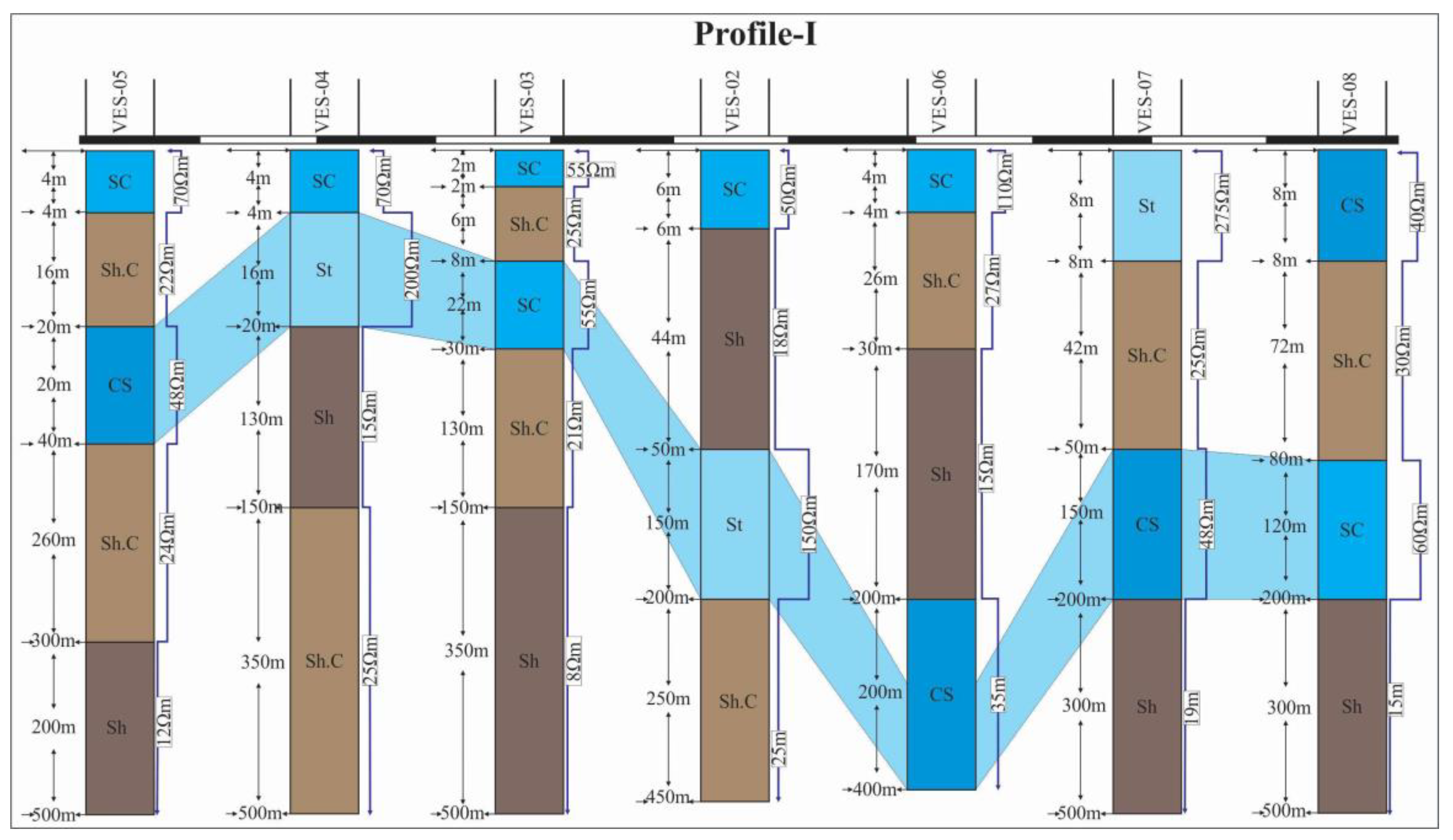
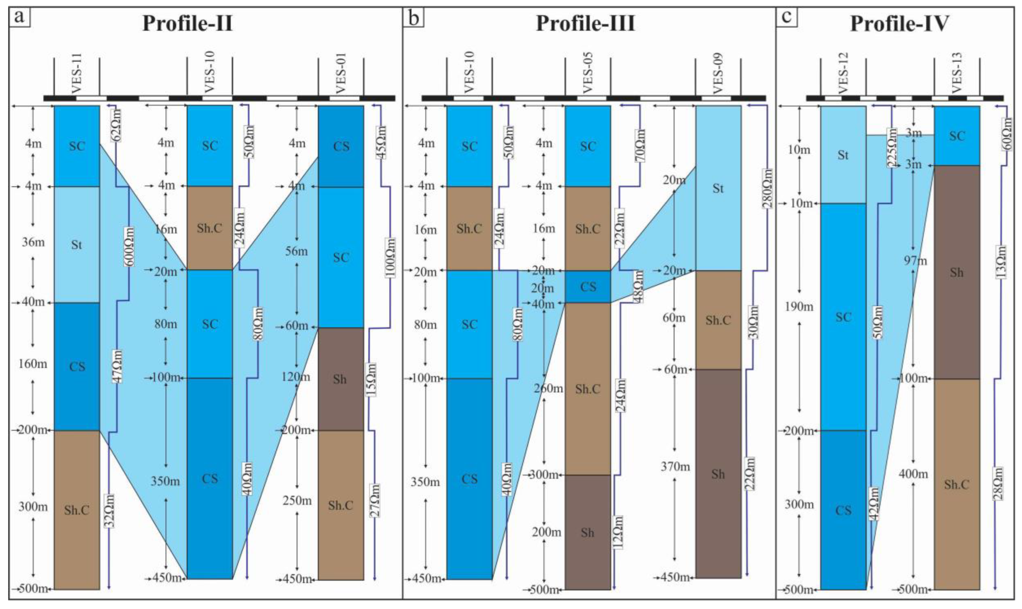
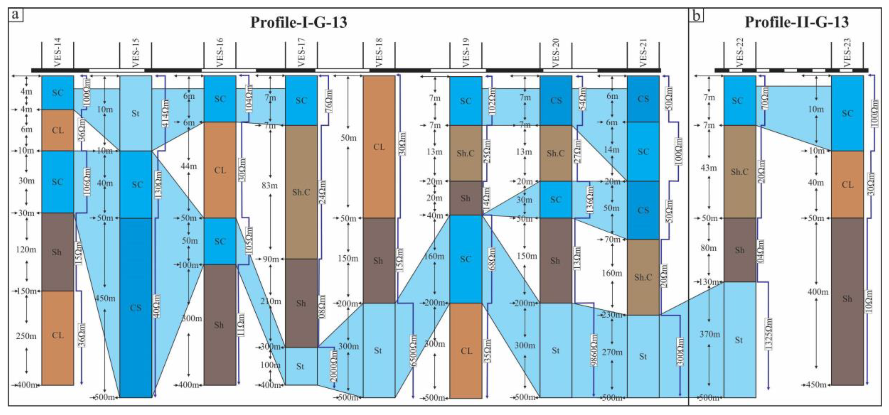
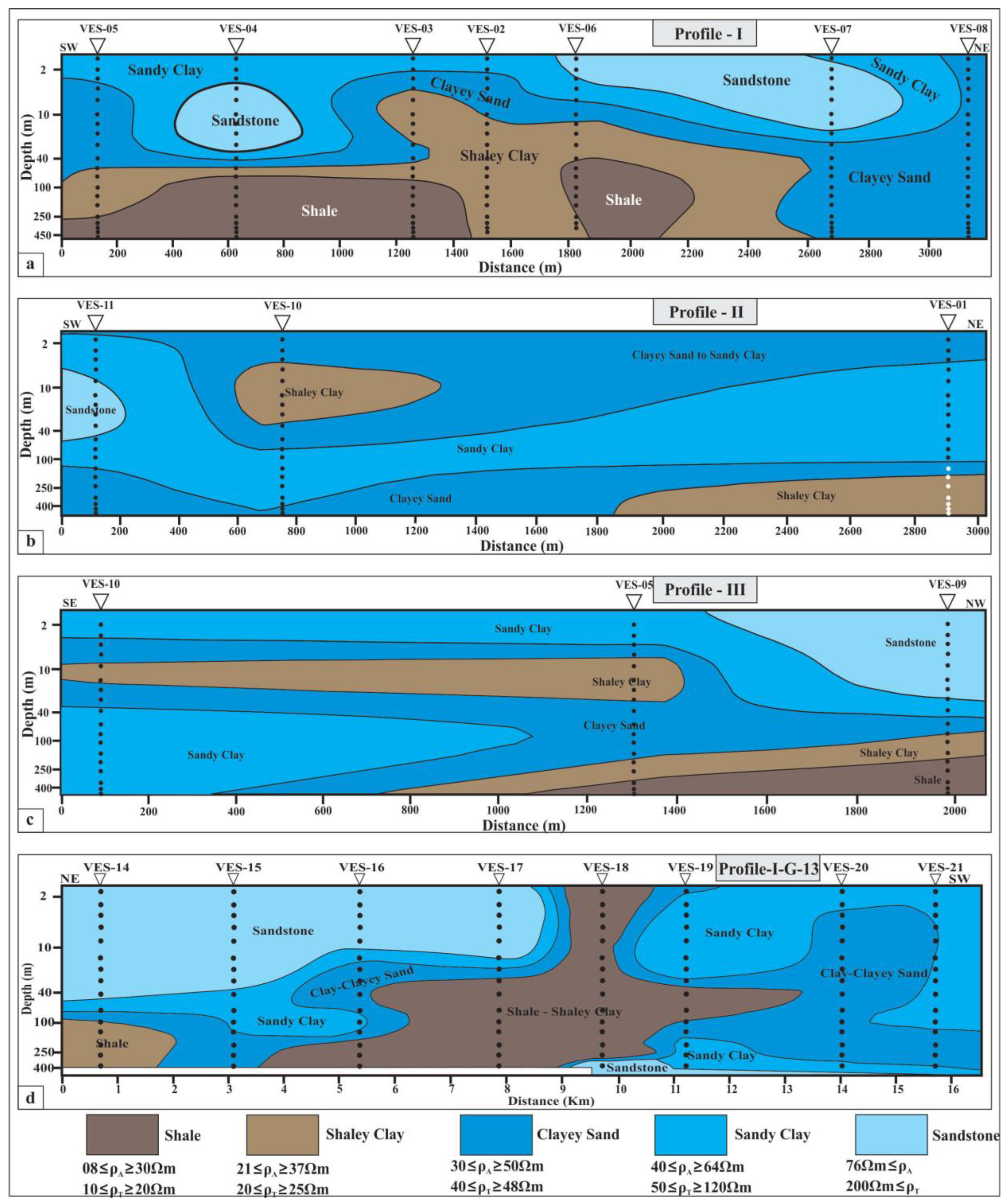
4.1. Geoelectrical Litho Section (GELS)
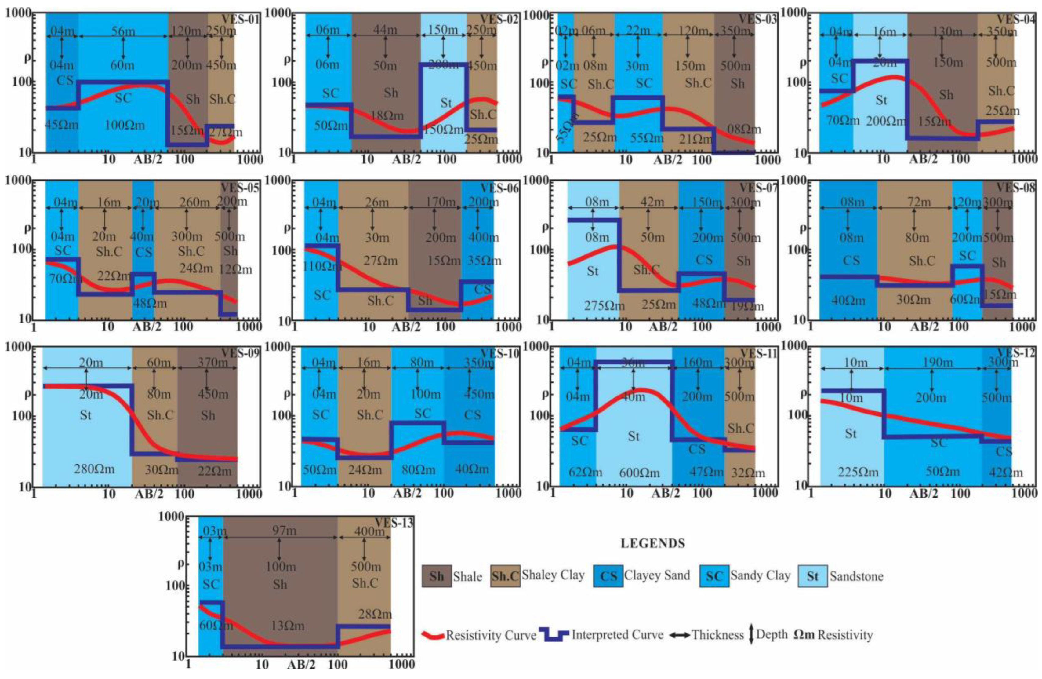
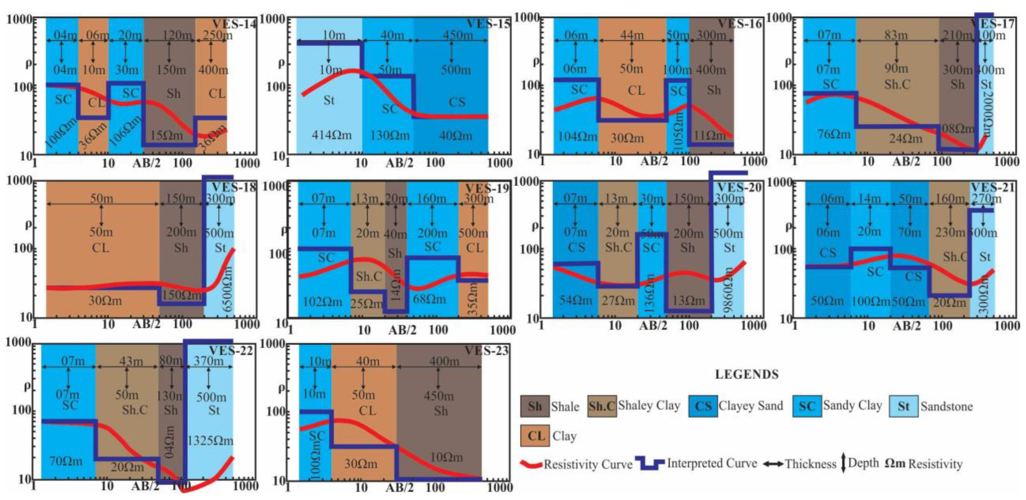
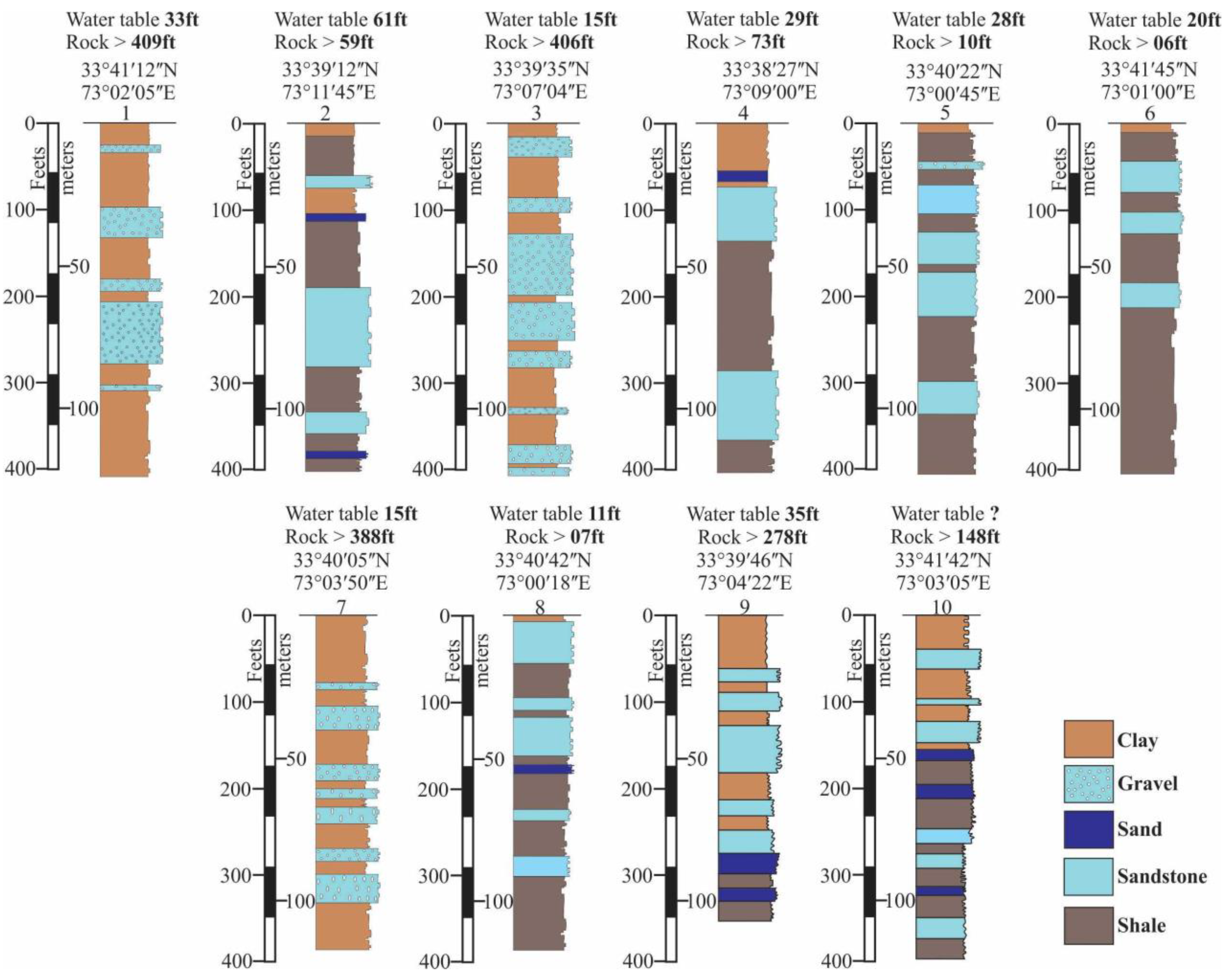
4.2. Geoelectrical Lithological Logs (GELL)
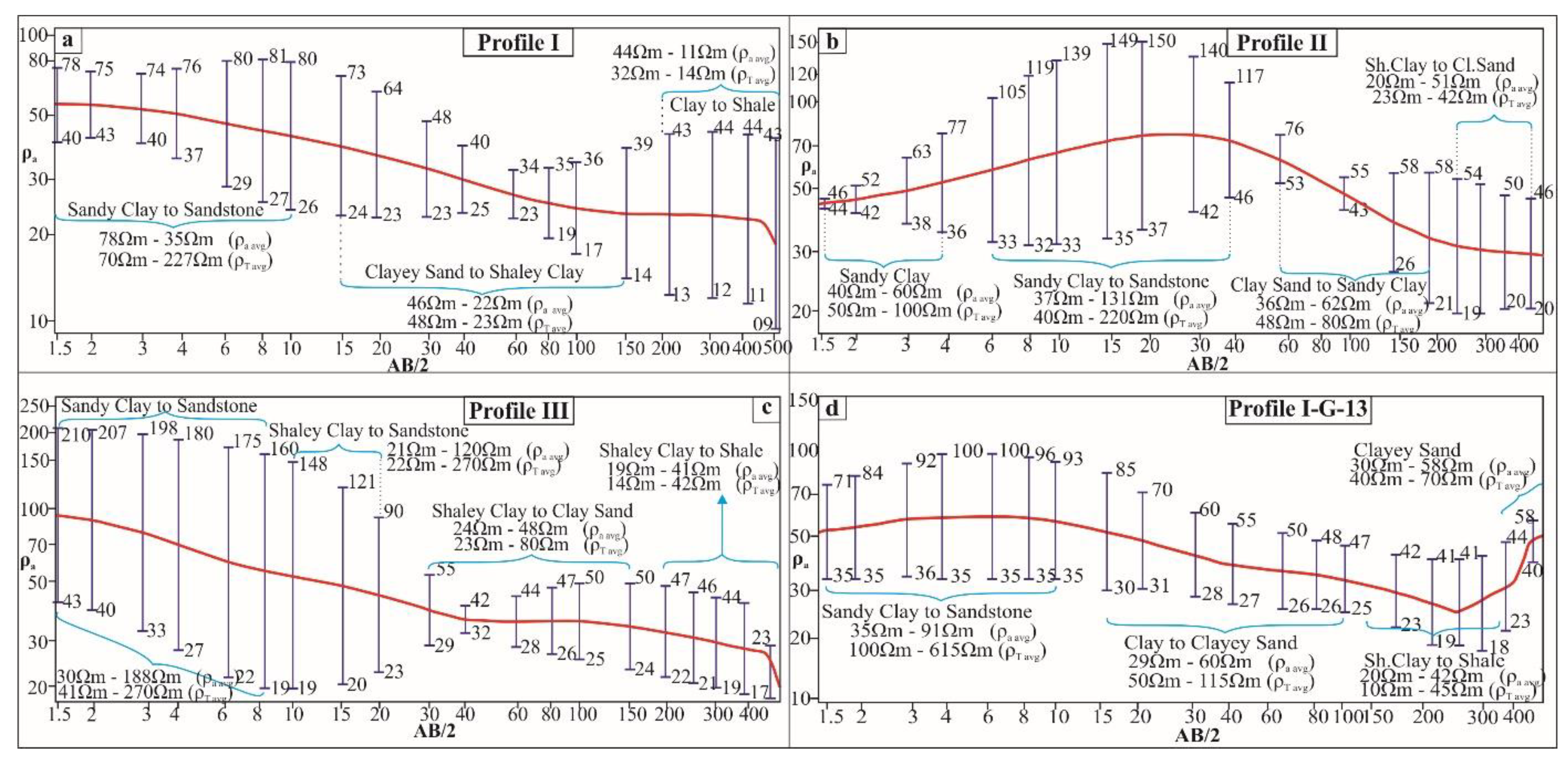
4.3. Pseudosection of Apparent Resistivity
4.4. Statistical Distribution of Resistivity
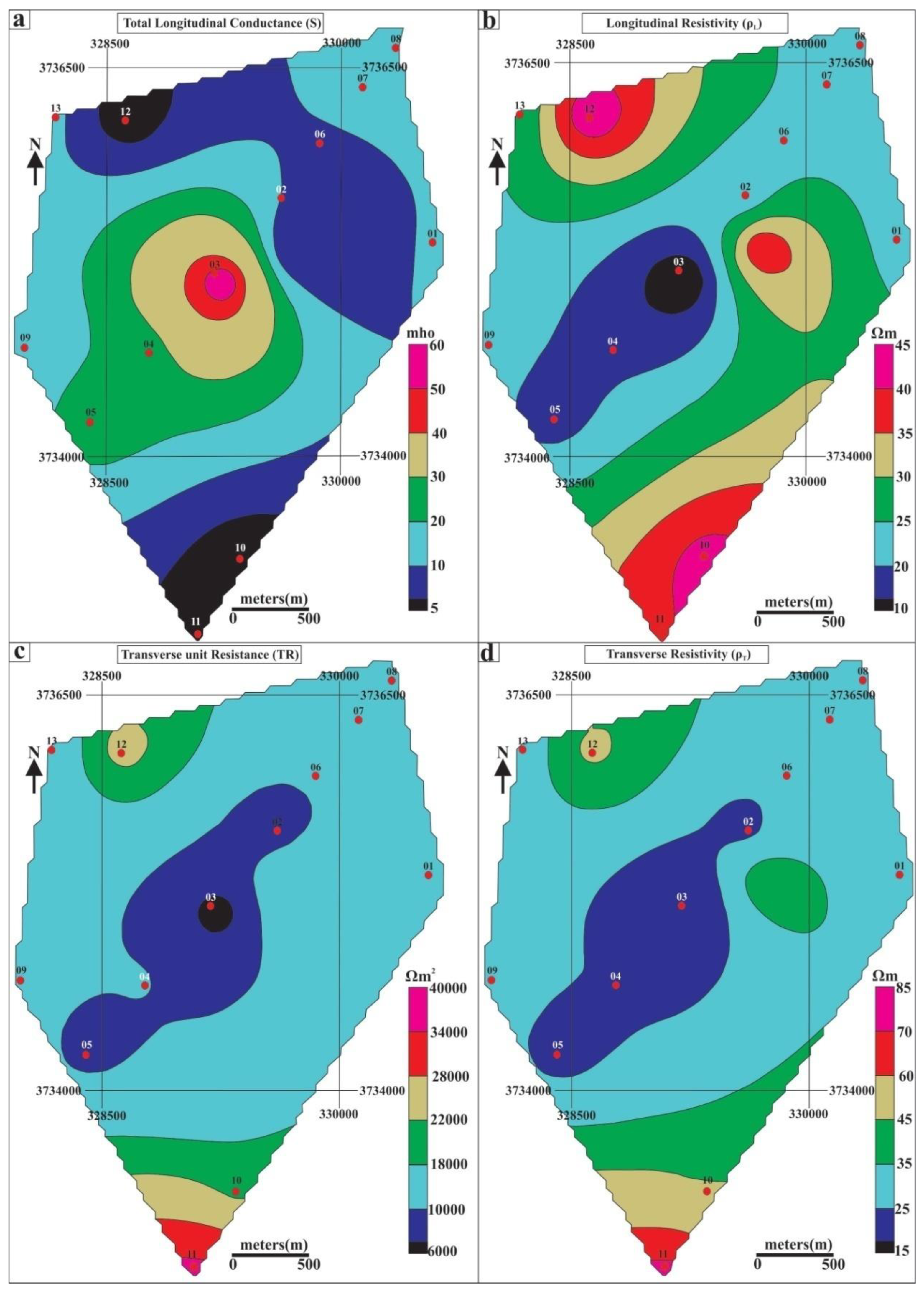
4.5. Dr Zarrouk of Hydraulic Parameters
4.5.1. Area 1
4.5.2. Area 2
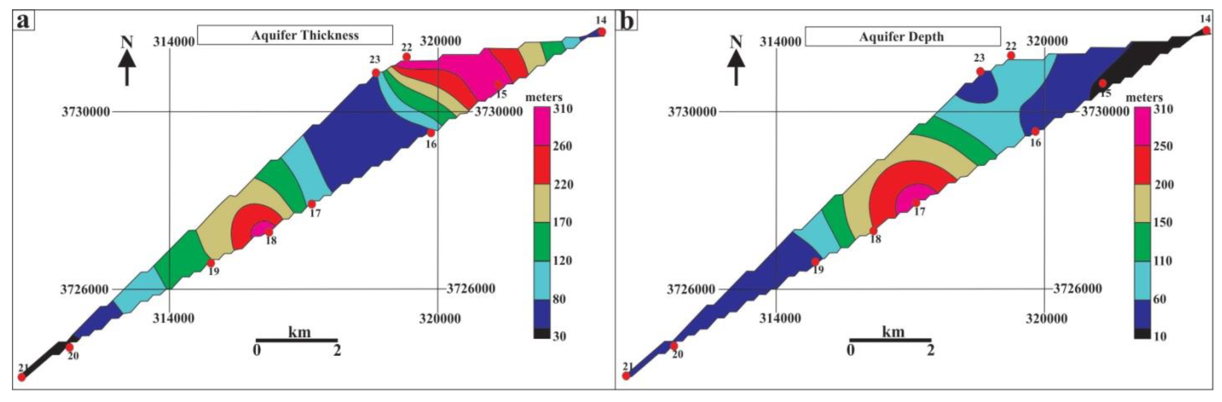
4.6. Aquifer Thickness vs. Depth
5. Conclusions
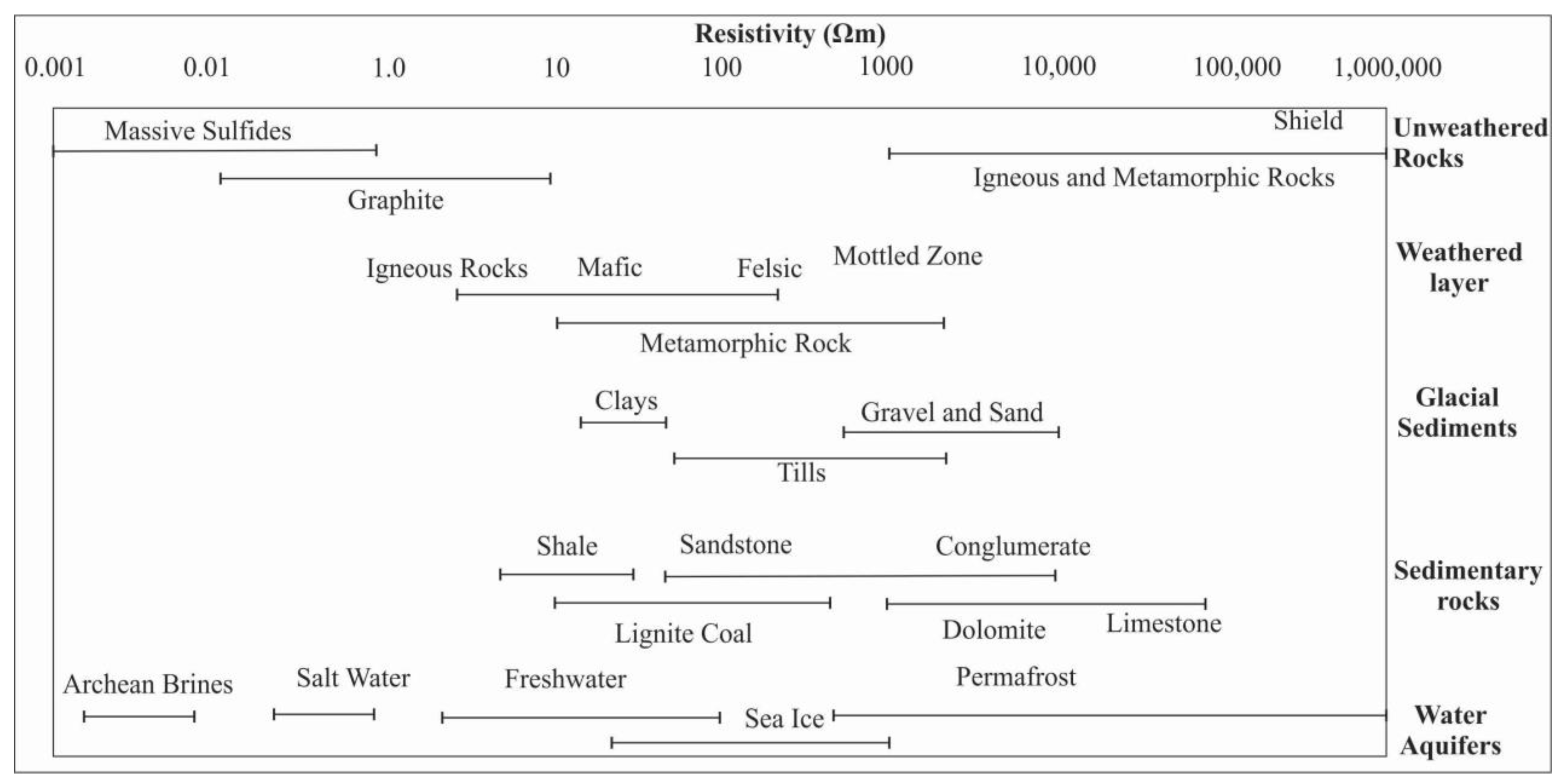
- The resistivity logs reveal the presence of various lithological units, including sandstone, shale, clay, sandy clay, clayey sand, and shaley clay. The main potential aquifer horizons are identified as sandstone, sandy clay, and clayey sand, while shaley clay appears to be a shallow aquifer of poor quality.
- The detailed geologs of Area 1 (Bara Kahu) and Area 2 (Aabpara to G13) indicate the presence of both shallow and deeper aquifers, with sandstone and sandy clay dominating at different depths. The P-I logs show shallow aquifers at 10–20 m depth and deeper aquifers at depths greater than 50 m. P-II logs reveal the presence of unconfined aquifers with clayey sand as the shallow aquifer and deeper aquifers consisting of sandy clay. P-III logs indicate the dominance of semi-confined aquifers with shallow potential in sandstone and sandy clay and deeper horizons in clayey sand.
- The pseudosections of both areas highlight good potential for groundwater, with various aquifer types and depths ranging from 10 to 40 m. The NE side of the study areas consistently shows better aquifer potential compared to the SW side, owing to the presence of maximum sandstone.
- The resistivity data and true resistivity sections further support the presence of distinct lithological units, with sandy beds dominating along the NE and NW sides, while clay/shale is prevalent in the SE–SW region.
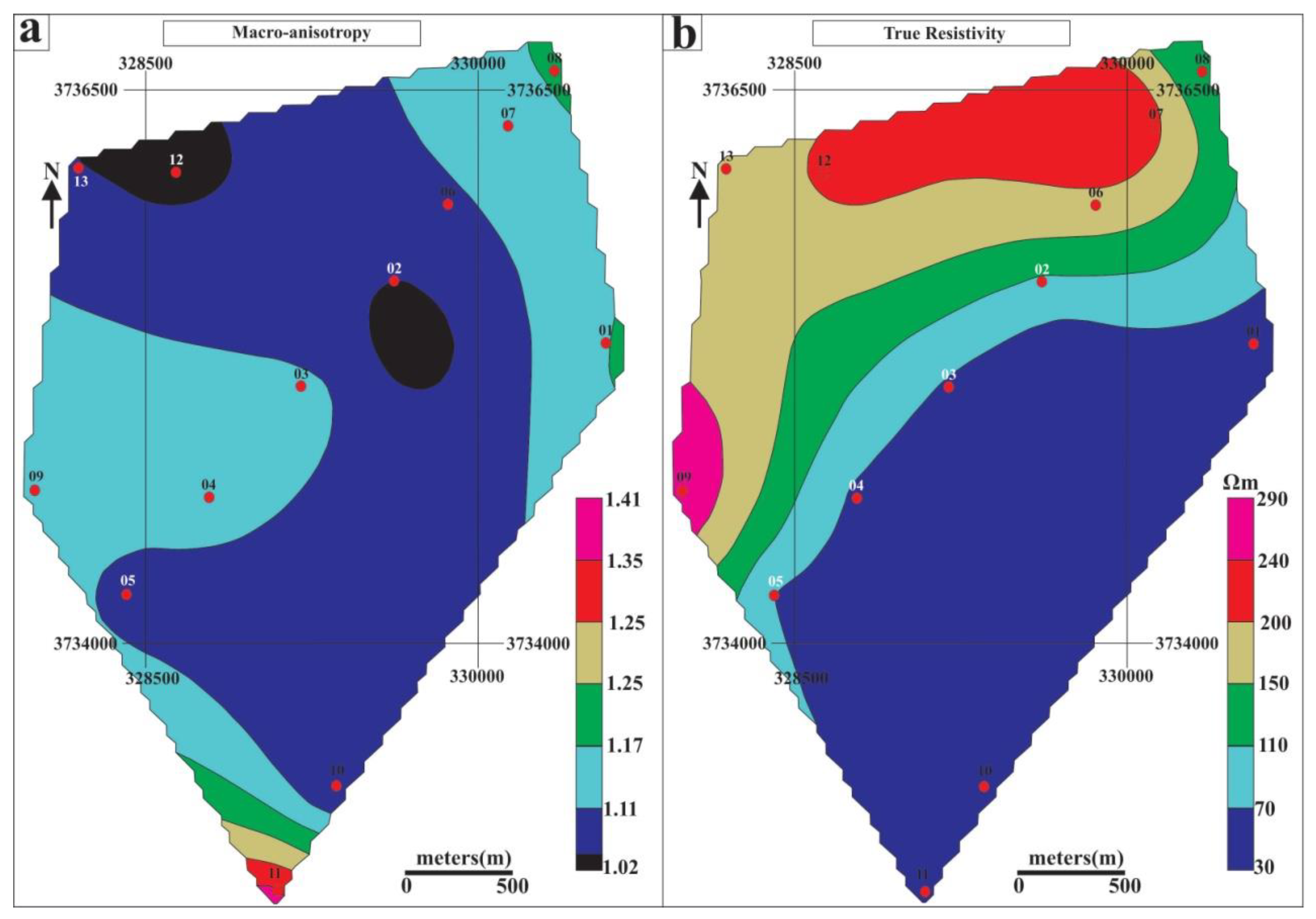
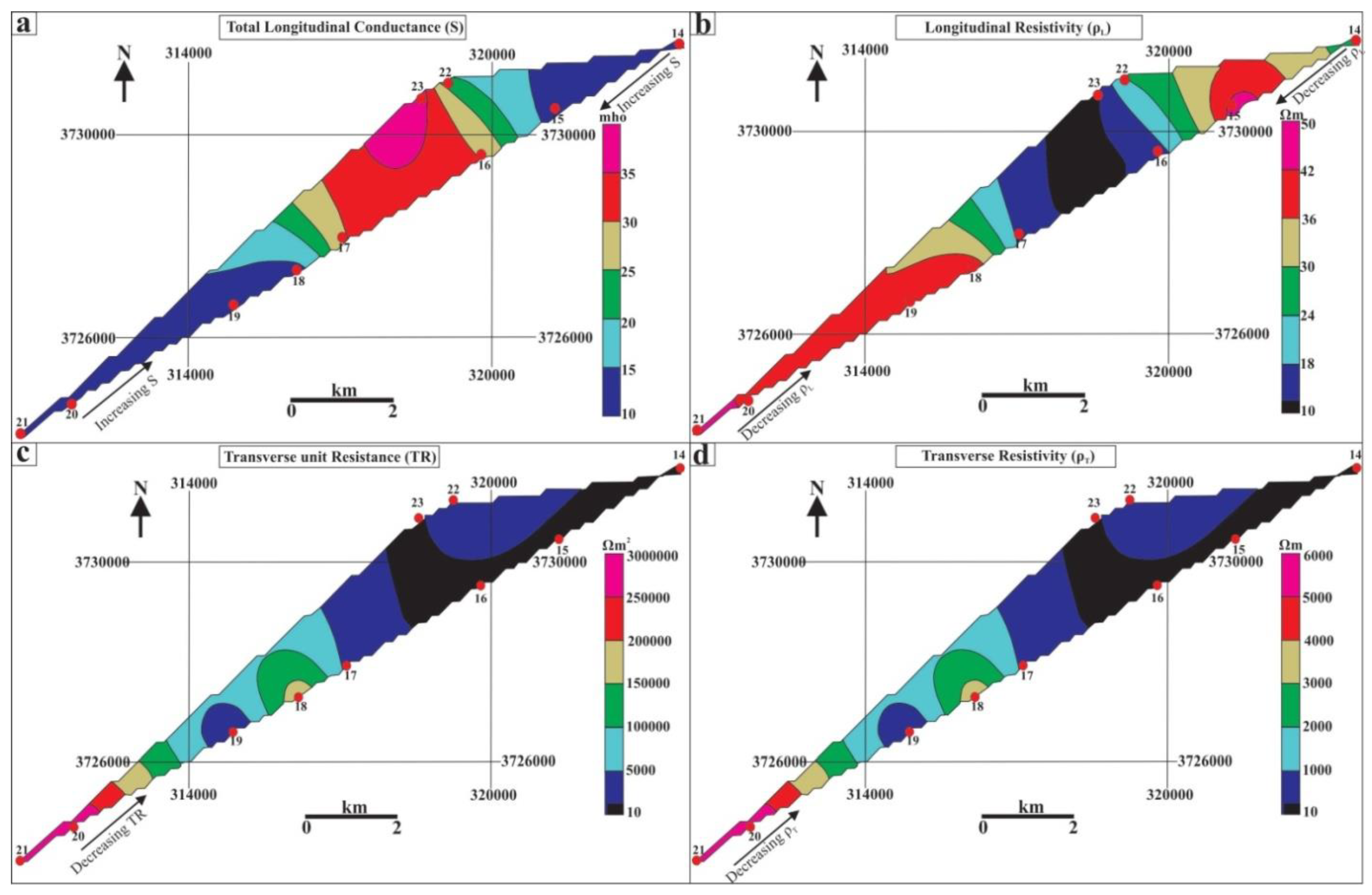
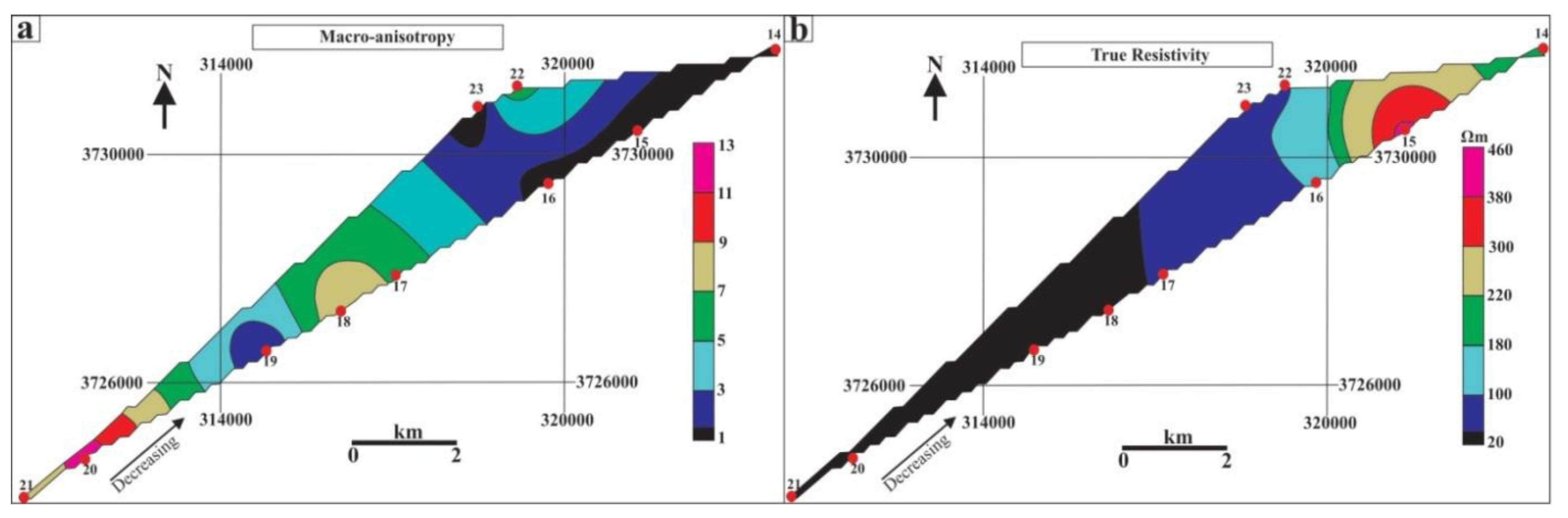
- The longitudinal conductance (S) and longitudinal resistivity (ρL) analyses confirm the presence of sandy units with good aquifer potential along the NW and SE sides. Transverse resistance (TR) and transverse resistivity (ρT) indicate the presence of permeable units along the NW and SE sides, while impermeable units dominate the SW side. The macroanisotropy and true resistivity maps provide additional evidence of lithological variations, with NE and SW sides showing different hydrological units.
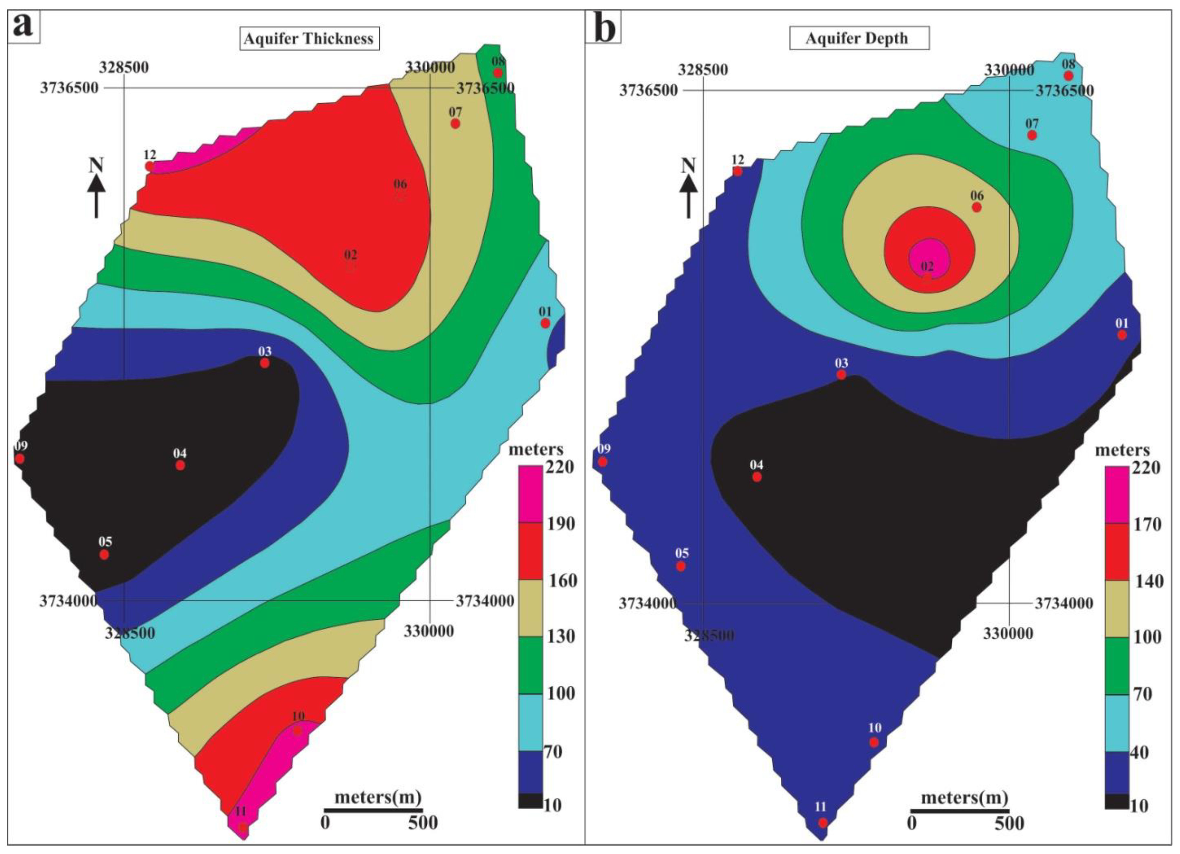
- The aquifer thickness and depth maps show variations in aquifer thickness ranging from 10 to 200 m, with maximum thickness recorded along the SE and NW sides, while the NE side exhibits greater depth. These maps highlight the SE side as a promising area for potential reservoirs.
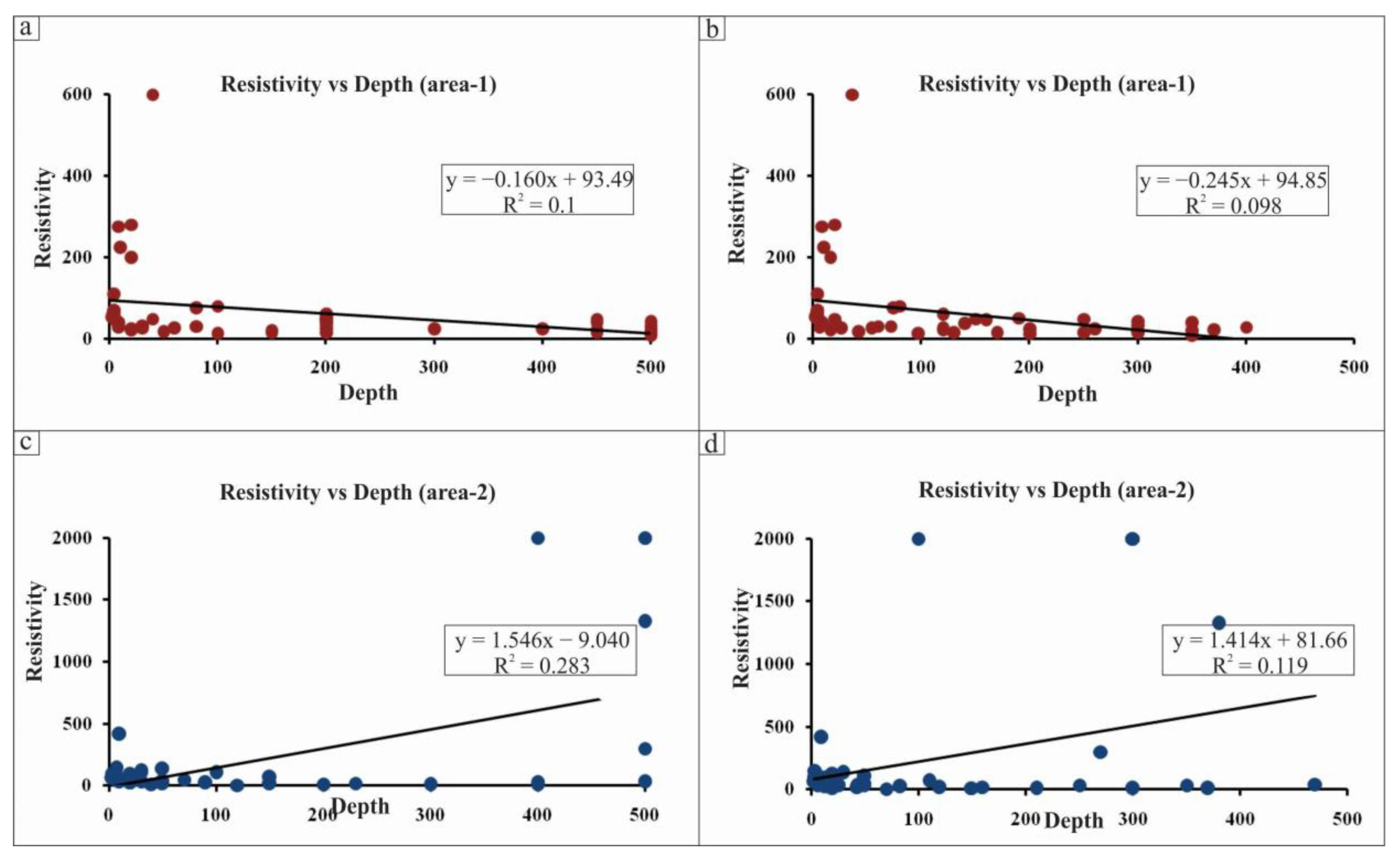
- The linear regression analysis suggests that depth and thickness have a relatively minor influence, accounting for only 10% to 20% of the resistivity variation. The major controlling factors on resistivity are groundwater characteristics, permeability, porosity, and lithological units, which account for 80% to 90% of the observed resistivity changes.
6. Recommendations
Author Contributions
Funding
Data Availability Statement
Acknowledgments
Conflicts of Interest
References
- Yan, D.; Yao, M.; Ludwig, F.; Kabat, P.; Huang, H.Q.; Hutjes, R.W.; Werners, S.E. Exploring future water shortage for large river basins under different water allocation strategies. Water Resour. Manag. 2018, 32, 3071–3086. [Google Scholar] [CrossRef]
- Oki, T.; Kanae, S. Global hydrological cycles and world water resources. Science 2006, 313, 1068–1072. [Google Scholar] [CrossRef] [PubMed]
- Plummer, C.C.; Carlson, D.; Hammersley, L. Physical Geology; McGraw-Hill/Education: New York, NY, USA, 2016. [Google Scholar]
- Casper, J.K. Water and Atmosphere: The Lifeblood of Natural Systems; Infobase Publishing: New York, NY, USA, 2007. [Google Scholar]
- Orimoloye, I.R.; Belle, J.A.; Olusola, A.O.; Busayo, E.T.; Ololade, O.O. Spatial assessment of drought disasters, vulnerability, severity and water shortages: A potential drought disaster mitigation strategy. Nat. Hazards 2021, 105, 2735–2754. [Google Scholar] [CrossRef]
- Salehi, M. Global water shortage and potable water safety; Today’s concern and tomorrow’s crisis. Environ. Int. 2022, 158, 106936. [Google Scholar] [CrossRef]
- López-Pacheco, I.Y.; Silva-Núñez, A.; Salinas-Salazar, C.; Arévalo-Gallegos, A.; Lizarazo-Holguin, L.A.; Barceló, D.; Iqbal, H.M.; Parra-Saldívar, R. Anthropogenic contaminants of high concern: Existence in water resources and their adverse effects. Sci. Total Environ. 2019, 690, 1068–1088. [Google Scholar] [CrossRef]
- Li, P.; Karunanidhi, D.; Subramani, T.; Srinivasamoorthy, K. Sources and consequences of groundwater contamination. Arch. Environ. Contam. Toxicol. 2021, 80, 1–10. [Google Scholar] [CrossRef]
- Carrard, N.; Foster, T.; Willetts, J. Groundwater as a source of drinking water in southeast Asia and the Pacific: A multi-country review of current reliance and resource concerns. Water 2019, 11, 1605. [Google Scholar] [CrossRef]
- Zhang, Z.; Wang, W. Managing aquifer recharge with multi-source water to realize sustainable management of groundwater resources in Jinan, China. Environ. Sci. Pollut. Res. 2021, 28, 10872–10888. [Google Scholar] [CrossRef]
- Zhang, Z.; Li, Y.; Wang, X.; Liu, Y.; Tang, W.; Ding, W.; Han, Q.; Shang, G.; Wang, Z.; Chen, K. Investigating River health across mountain to urban transitions using Pythagorean fuzzy cloud technique under uncertain environment. J. Hydrol. 2023, 620, 129426. [Google Scholar] [CrossRef]
- Sarah, S.; Ahmed, S.; Violette, S.; de Marsily, G. Groundwater sustainability challenges revealed by quantification of contaminated groundwater volume and aquifer depletion in hard rock aquifer systems. J. Hydrol. 2021, 597, 126286. [Google Scholar] [CrossRef]
- Brindha, K.; Schneider, M. Impact of urbanization on groundwater quality. In GIS and Geostatistical Techniques for Groundwater Science; Elsevier: Amsterdam, The Netherlands, 2019; pp. 179–196. [Google Scholar]
- Karunanidhi, D.; Subramani, T.; Srinivasamoorthy, K.; Yang, Q. Environmental chemistry, toxicity and health risk assessment of groundwater: Environmental persistence and management strategies. Environ. Res. 2022, 214, 113884. [Google Scholar] [CrossRef]
- Akhtar, N.; Syakir Ishak, M.I.; Bhawani, S.A.; Umar, K. Various natural and anthropogenic factors responsible for water quality degradation: A review. Water 2021, 13, 2660. [Google Scholar] [CrossRef]
- Rao, P.S.C.; Jawitz, J.W.; Enfield, C.G.; Falta, R., Jr.; Annable, M.D.; Wood, A.L. Technology integration for contaminated site remediation: Clean-up goals and performance criteria. Groundw. Qual. Nat. Enhanc. Restor. Groundw. Pollut. 2001, 275, 571–578. [Google Scholar]
- Khorrami, M.; Malekmohammadi, B. Effects of excessive water extraction on groundwater ecosystem services: Vulnerability assessments using biophysical approaches. Sci. Total Environ. 2021, 799, 149304. [Google Scholar] [CrossRef]
- Díaz-Alcaide, S.; Martínez-Santos, P. Advances in groundwater potential mapping. Hydrogeol. J. 2019, 27, 2307–2324. [Google Scholar] [CrossRef]
- Zaher, M.A.; Younis, A.; Shaaban, H.; Mohamaden, M.I. Integration of geophysical methods for groundwater exploration: A case study of El Sheikh Marzouq area, Farafra Oasis, Egypt. Egypt. J. Aquat. Res. 2021, 47, 239–244. [Google Scholar] [CrossRef]
- Lubang, J.; Liu, H.; Chen, R. Combined Application of Hydrogeological and Geoelectrical Study in Groundwater Exploration in Karst-Granite Areas, Jiangxi Province. Water 2023, 15, 865. [Google Scholar] [CrossRef]
- Mohamed, A.; Othman, A.; Galal, W.F.; Abdelrady, A. Integrated geophysical approach of groundwater potential in Wadi Ranyah, Saudi Arabia, using gravity, electrical resistivity, and remote-sensing techniques. Remote Sens. 2023, 15, 1808. [Google Scholar] [CrossRef]
- Nagaiah, E.; Sonkamble, S.; Chandra, S. Electrical geophysical techniques pin-pointing the bedrock fractures for groundwater exploration in granitic hard rocks of Southern India. J. Appl. Geophys. 2022, 199, 104610. [Google Scholar] [CrossRef]
- Aliou, A.-S.; Dzikunoo, E.A.; Yidana, S.M.; Loh, Y.; Chegbeleh, L.P. Investigation of Geophysical Signatures for Successful Exploration of Groundwater in Highly Indurated Sedimentary Basins: A Look at the Nasia Basin, NE Ghana. Nat. Resour. Res. 2022, 31, 3223–3251. [Google Scholar] [CrossRef]
- Bhatnagar, S.; Taloor, A.K.; Roy, S.; Bhattacharya, P. Delineation of aquifers favorable for groundwater development using Schlumberger configuration resistivity survey techniques in Rajouri district of Jammu and Kashmir, India. Groundw. Sustain. Dev. 2022, 17, 100764. [Google Scholar] [CrossRef]
- Brahmi, S.; Baali, F.; Hadji, R.; Brahmi, S.; Hamad, A.; Rahal, O.; Zerrouki, H.; Saadali, B.; Hamed, Y. Assessment of groundwater and soil pollution by leachate using electrical resistivity and induced polarization imaging survey, case of Tebessa municipal landfill, NE Algeria. Arab. J. Geosci. 2021, 14, 249. [Google Scholar] [CrossRef]
- Islami, N.; Irianti, M.; Fakhruddin, F.; Azhar, A.; Nor, M. Application of geoelectrical resistivity method for the assessment of shallow aquifer quality in landfill areas. Environ. Monit. Assess. 2020, 192, 249. [Google Scholar] [CrossRef] [PubMed]
- Chibuike, A.; Chukwu, A.C.; Kelechi, O.K. Efficiency and limitation of vertical electrical sounding in evaluation of groundwater potential in fractured shale terrain: A case study of Abakaliki Area Lower Benue Trough Nigeria. Environ. Monit. Assess. 2023, 195, 158. [Google Scholar] [CrossRef]
- Joel, E.S.; Olasehinde, P.I.; Adagunodo, T.A.; Omeje, M.; Oha, I.; Akinyemi, M.L.; Olawole, O.C. Geo-investigation on groundwater control in some parts of Ogun state using data from Shuttle Radar Topography Mission and vertical electrical soundings. Heliyon 2020, 6, e03327. [Google Scholar] [CrossRef] [PubMed]
- Soomro, A.; Qureshi, A.L.; Jamali, M.A.; Ashraf, A. Groundwater investigation through vertical electrical sounding at hilly area from Nooriabad toward Karachi. Acta Geophys. 2019, 67, 247–261. [Google Scholar] [CrossRef]
- Omeje, E.T.; Ugbor, D.O.; Ibuot, J.C.; Obiora, D.N. Assessment of groundwater repositories in Edem, Southeastern Nigeria, using vertical electrical sounding. Arab. J. Geosci. 2021, 14, 421. [Google Scholar] [CrossRef]
- de Almeida, A.; Maciel, D.F.; Sousa, K.F.; Nascimento, C.T.C.; Koide, S. Vertical electrical sounding (VES) for estimation of hydraulic parameters in the porous aquifer. Water 2021, 13, 170. [Google Scholar] [CrossRef]
- Rashid, M.; Ahmad, W.; Zeb, M.J.; Haider, N.; Khan, A.; Khan, S. Determination of Underground Structure and Migration of Hot Plumes Contaminating Fresh Water Using Vertical Electrical Survey (VES) and Magnetic Survey, A Case Study of Tattapani Thermal Spring, Azad Kashmir. Int. J. Econ. Environ. Geol. 2019, 10, 84–92. [Google Scholar]
- Akinrinade, O.J.; Adesina, R.B. Hydrogeophysical investigation of groundwater potential and aquifer vulnerability prediction in basement complex terrain–A case study from Akure, Southwestern Nigeria. Mater. Geoenviron. 2016, 63, 55–66. [Google Scholar] [CrossRef]
- Sanuade, O.A.; Arowoogun, K.I.; Amosun, J.O. A review on the use of geoelectrical methods for characterization and monitoring of contaminant plumes. Acta Geophys. 2022, 70, 2099–2117. [Google Scholar] [CrossRef]
- Kumar, D.; Mondal, S.; Warsi, T. Deep insight to the complex aquifer and its characteristics from high resolution electrical resistivity tomography and borehole studies for groundwater exploration and development. J. Earth Syst. Sci. 2020, 129, 68. [Google Scholar] [CrossRef]
- Lee, S.C.H.; Noh, K.A.M.; Zakariah, M.N.A. High-resolution electrical resistivity tomography and seismic refraction for groundwater exploration in fracture hard rocks: A case study in Kanthan, Perak, Malaysia. J. Asian Earth Sci. 2021, 218, 104880. [Google Scholar] [CrossRef]
- Hussain, Z.; Wang, Z.; Wang, J.; Yang, H.; Arfan, M.; Hassan, D.; Wang, W.; Azam, M.I.; Faisal, M. A comparative appraisal of classical and holistic water scarcity indicators. Water Resour. Manag. 2022, 36, 931–950. [Google Scholar] [CrossRef]
- Qureshi, A.S. Groundwater Governance in Pakistan: From Colossal Development to Neglected Management. Water 2020, 12, 3017. [Google Scholar] [CrossRef]
- Ahmed, K.; Shamsuddin, S.; Demirel, M.C.; Nadeem, N.; Najeebullah, K. The changing characteristics of groundwater sustainability in Pakistan from 2002 to 2016. Hydrogeol. J. 2019, 27, 2485–2496. [Google Scholar] [CrossRef]
- Ebrahim, Z.T. Is Pakistan Running Dry? Water Issues in Himalayan South Asia: Internal Challenges, Disputes and Transboundary Tensions; Springer: Berlin/Heidelberg, Germany, 2020; pp. 153–181. [Google Scholar]
- Iqbal, A.R. Water Shortage in Pakistan-A Crisis around the Corner. Inst. Strateg. Stud. Res. Anal. (ISSRA) 2010, 2, 1–13. [Google Scholar]
- Briscoe, J.; Qamar, U.; Contijoch, M.; Amir, P.; Blackmore, D. Pakistan’s Water Economy: Running Dry; Oxford University Press: Karachi, Pakistan, 2006. [Google Scholar]
- Saleem, S.; Ali, W.; Afzal, M.S. Status of Drinking Water Quality and its Contamination in Pakistan. J. Environ. Res. 2018, 2, 6. [Google Scholar]
- Daud, M.; Nafees, M.; Ali, S.; Rizwan, M.; Bajwa, R.A.; Shakoor, M.B.; Arshad, M.U.; Chatha, S.A.S.; Deeba, F.; Murad, W. Drinking water quality status and contamination in Pakistan. BioMed Res. Int. 2017, 2017, 7908183. [Google Scholar] [CrossRef]
- Nabeela, F.; Azizullah, A.; Bibi, R.; Uzma, S.; Murad, W.; Shakir, S.K.; Ullah, W.; Qasim, M.; Häder, D.-P. Microbial contamination of drinking water in Pakistan—A review. Environ. Sci. Pollut. Res. 2014, 21, 13929–13942. [Google Scholar] [CrossRef]
- Force, Water Sector Task. A Productive and Water-Secure Pakistan: Infrastructure, Institutions, Strategy, the Report of the Water Sector Task Force of the Friends of Democratic Pakistan; Force, Water Sector Task: Islamabad, Pakistan, 2012. [Google Scholar]
- Iqbal, N.; Din, S.; Ashraf, M.; Asmat, S. Hydrological Assessment of Surface and Groundwater Resources of Islamabad, Pakistan. Pak. Counc. Res. Water Resour. (PCRWR) Islamabad 2023, 76. [Google Scholar]
- Sohail, M.T.; Mahfooz, Y.; Azam, K.; Yen, Y.; Genfu, L.; Fahad, S. Impacts of urbanization and land cover dynamics on underground water in Islamabad, Pakistan. Desalin Water Treat 2019, 159, 402–411. [Google Scholar] [CrossRef]
- Khan, J.; Ren, X.; Hussain, M.A.; Jan, M.Q. Monitoring Land Subsidence Using PS-InSAR Technique in Rawalpindi and Islamabad, Pakistan. Remote Sens. 2022, 14, 3722. [Google Scholar] [CrossRef]
- Hassan, D.; Rais, M.N.; Ahmed, W.; Bano, R.; Burian, S.J.; Ijaz, M.W.; Bhatti, F.A. Future water demand modeling using water evaluation and planning: A case study of the Indus Basin in Pakistan. Sustain. Water Resour. Manag. 2019, 5, 1903–1915. [Google Scholar] [CrossRef]
- Khan, U.; Janjuhah, H.T.; Kontakiotis, G.; Rehman, A.; Zarkogiannis, S.D. Natural Processes and Anthropogenic Activity in the Indus River Sedimentary Environment in Pakistan: A Critical Review. J. Mar. Sci. Eng. 2021, 9, 1109. [Google Scholar] [CrossRef]
- Water Resource Division, M.O.W.R. National Water Policy. Policy Div. 2018, 1–44. [Google Scholar]
- Shah, S.H.I.A.; Jianguo, Y.; Jahangir, Z.; Tariq, A.; Aslam, B. Integrated geophysical technique for groundwater salinity delineation, an approach to agriculture sustainability for Nankana Sahib Area, Pakistan. Geomat. Nat. Hazards Risk 2022, 13, 1043–1064. [Google Scholar] [CrossRef]
- Fajana, A. Integrated geophysical investigation of aquifer and its groundwater potential in phases 1 and 2, Federal University Oye-Ekiti, south-western basement complex of Nigeria. Model. Earth Syst. Environ. 2020, 6, 1707–1725. [Google Scholar] [CrossRef]
- Echogdali, F.Z.; Boutaleb, S.; Bendarma, A.; Saidi, M.E.; Aadraoui, M.; Abioui, M.; Ouchchen, M.; Abdelrahman, K.; Fnais, M.S.; Sajinkumar, K.S. Application of analytical hierarchy process and geophysical method for groundwater potential mapping in the Tata basin, Morocco. Water 2022, 14, 2393. [Google Scholar] [CrossRef]
- Ahmed, Z.; Ansari, M.T.; Zahir, M.; Shakir, U.; Subhan, M. Hydrogeophysical investigation for groundwater potential through Electrical Resistivity Survey in Islamabad, Pakistan. J. Geogr. Soc. Sci. JGSS 2020, 2, 147–163. [Google Scholar]
- Qadir, A.; Amjad, M.R.; Khan, T.; Zafar, M.; Hasham, M.; Khan, U.A.; Khattak, S.A.; Ahmad, I. Demarcation of groundwater potential zones by electrical resistivity survey (ERS) islamabad, Pakistan. Int. J. Econ. Environ. Geol. 2018, 9, 39–44. [Google Scholar]
- Lisa, M.; Khan, S.A.; Khwaja, A.A. Focal mechanism study of north Potwar deformed zone, Pakistan. Acta Seismol. Sin. 2004, 17, 255–261. [Google Scholar] [CrossRef]
- Khan, S.; Waseem, M.; Khan, M.A. A Seismic Hazard Map Based on Geology and Shear-wave Velocity in Rawalpindi–Islamabad, Pakistan. Acta Geol. Sin. Engl. Ed. 2021, 95, 659–673. [Google Scholar] [CrossRef]
- Adeel, M.B.; Nizamani, Z.A.; Aaqib, M.; Khan, S.; Rehman, J.U.; Bhusal, B.; Park, D. Estimation of V S30 using shallow depth time-averaged shear wave velocity of Rawalpindi–Islamabad, Pakistan. Geomat. Nat. Hazards Risk 2023, 14, 1–21. [Google Scholar] [CrossRef]
- Shah, S.M.I. Stratigraphy of Pakistan, 22nd ed.; Geological Survey of Pakistan Publication Directorate: Quetta, Pakistan, 2009; Volume 22, p. 381.
- Sheikh, I.M.; Pasha, M.K.; Williams, V.S.; Raza, S.Q.; Khan, K.S. Environmental geology of the Islamabad-Rawalpindi area, northern Pakistan. In Regional Studies of the Potwar-Plateau Area, Northern Pakistan. Bull. G; U.S. Department of the Interior: Washington, DC, USA, 2008; Volume 2078. [Google Scholar]
- MonaLisa; Khwaja, A.A. Tectonic Model of NW Himalayan Fold and Thrust Belt on the basis of Focal Mechanism studies. Pak. J. Meteorol. 2005, 2, 9–50. [Google Scholar]
- Williams, V.S.; Pasha, M.K.; Sheikh, I.M. Geologic Map of the Islamabad-Rawalpindi Area, Punjab, Northern Pakistan; The Survey; USGS: Reston, VA, USA, 1999. Available online: https://pubs.usgs.gov/publication/ofr9947 (accessed on 19 November 2023).
- Shah, S.H.; Khan, N.A.; Bhatti, M.A. Geological Map of Islamabad and surrounding. In Geological Survey of Pakistan Special Map Series No. 1; Geological Survey of Pakistan: Quetta, Pakistan, 2000. [Google Scholar]
- Rashid, M.; Ahmed, W.; Anwar, S.; Abbas, S.A.; Waseem, M.; Khan, S. Groundwater resource characterization using geo-electrical survey: A case study of Rawlakot, Azad Jammu and Kashmir. J. Himal. Earth Sci. 2017, 50, 125–136. [Google Scholar]
- Gómez, D.G.; Ochoa, C.G.; Godwin, D.; Tomasek, A.A.; Zamora Re, M.I. Soil Water Balance and Shallow Aquifer Recharge in an Irrigated Pasture Field with Clay Soils in the Willamette Valley, Oregon, USA. Hydrology 2022, 9, 60. [Google Scholar] [CrossRef]
- Islam, I.; Ahmed, W.; Rashid, M.U.; Orakzai, A.U.; Ditta, A. Geophysical and geotechnical characterization of shallow subsurface soil: A case study of University of Peshawar and surrounding areas. Arab. J. Geosci. 2020, 13, 949. [Google Scholar] [CrossRef]
- Oyeyemi, K.D.; Aizebeokhai, A.P.; Metwaly, M.; Omobulejo, O.; Sanuade, O.A.; Okon, E.E. Assessing the suitable electrical resistivity arrays for characterization of basement aquifers using numerical modeling. Heliyon 2022, 8, e09427. [Google Scholar] [CrossRef]
- Singh, U.; Sharma, P.K. Study on geometric factor and sensitivity of subsurface for different electrical resistivity Tomography Arrays. Arab. J. Geosci. 2022, 15, 560. [Google Scholar] [CrossRef]
- Mirzaei, L.; Hafizi, M.K.; Riahi, M.A. Application of Dipole–Dipole, Schlumberger, and Wenner–Schlumberger Arrays in Groundwater Exploration in Karst Areas Using Electrical Resistivity and IP Methods in a Semi-arid Area, Southwest Iran. In Water Resources in Arid Lands: Management and Sustainability; Springer: Berlin/Heidelberg, Germany, 2021; pp. 81–89. [Google Scholar]
- Bobachev, C. IPI2Win: A Windows Software for an Automatic Interpretation of Resistivity Sounding Data; Moscow State University: Moscow, Russia, 2002. [Google Scholar]
- Rashid, M.; Ahmed, W.; Zeb, M.J.; Mahmood, Z.; Khan, S.; Waseem, M. Geoelectrical and magnetic survey of Tatta Pani thermal spring: A case study from Kotli District, Jammu and Kashmir, Pakistan. Geomech. Geophys. Geo-Energy Geo-Resour. 2021, 7, 41. [Google Scholar] [CrossRef]
- Hasan, M.; Shang, Y.; Jin, W.; Akhter, G. Estimation of hydraulic parameters in a hard rock aquifer using integrated surface geoelectrical method and pumping test data in southeast Guangdong, China. Geosci. J. 2021, 25, 223–242. [Google Scholar] [CrossRef]
- Telford, W.M.; Geldart, L.P.; Sheriff, R.E. Applied Geophysics, 2nd ed.; Cambridge University Press: Cambridge, UK, 1990; Volume 1, p. 770. [Google Scholar]
- Metwaly, M.; Elawadi, E.; Moustafal, S.S.; Al Fouzan, F.; Mogren, S.; Al Arifi, N. Groundwater exploration using geoelectrical resistivity technique at Al-Quwy’yia area central Saudi Arabia. Int. J. Phys. Sci. 2012, 7, 317–326. [Google Scholar] [CrossRef]
- George, N.J. Modelling the trends of resistivity gradient in hydrogeological units: A case study of alluvial environment. Model. Earth Syst. Environ. 2021, 7, 95–104. [Google Scholar] [CrossRef]
- Ghani, M.; Atif, M.; Saeed, M.; Rasheed, M.; Abbas, S.A.; Jan, I.U.; Aziz, M. Geo-electrical sounding for subsurface lithological investigation and modeling for groundwater exploration in Sheikhmanda Kili region, Northern Quetta, Pakistan. Himal Geol 2022, 43, 40–50. [Google Scholar]
- Mainoo, P.A.; Manu, E.; Yidana, S.M.; Agyekum, W.A.; Stigter, T.; Duah, A.A.; Preko, K. Application of 2D-Electrical resistivity tomography in delineating groundwater potential zones: Case study from the voltaian super group of Ghana. J. Afr. Earth Sci. 2019, 160, 103618. [Google Scholar] [CrossRef]
- Magara, K. Comparison of porosity-depth relationships of shale and sandstone. J. Pet. Geol. 1980, 3, 175–185. [Google Scholar] [CrossRef]
- Scherer, M. Parameters influencing porosity in sandstones: A model for sandstone porosity prediction. AAPG Bull. 1987, 71, 485–491. [Google Scholar] [CrossRef]
- Mohammed, M.; Senosy, M.; Abudeif, A. Derivation of empirical relationships between geotechnical parameters and resistivity using electrical resistivity tomography (ERT) and borehole data at Sohag University site, upper Egypt. J. Afr. Earth Sci. 2019, 158, 103563. [Google Scholar] [CrossRef]
- Uhlemann, S.; Kuras, O.; Richards, L.A.; Naden, E.; Polya, D.A. Electrical resistivity tomography determines the spatial distribution of clay layer thickness and aquifer vulnerability, Kandal Province, Cambodia. J. Asian Earth Sci. 2017, 147, 402–414. [Google Scholar] [CrossRef]
- Nguyen, F.; Garambois, S.; Jongmans, D.; Pirard, E.; Loke, M. Image processing of 2D resistivity data for imaging faults. J. Appl. Geophys. 2005, 57, 260–277. [Google Scholar] [CrossRef]
- Singh, U.; Das, R.; Hodlur, G. Significance of Dar-Zarrouk parameters in the exploration of quality affected coastal aquifer systems. Environ. Geol. 2004, 45, 696–702. [Google Scholar] [CrossRef]
- Hasan, M.; Shang, Y.; Akhter, G.; Jin, W. Delineation of contaminated aquifers using integrated geophysical methods in Northeast Punjab, Pakistan. Environ. Monit. Assess. 2020, 192, 12. [Google Scholar] [CrossRef]
- Mahmud, S.; Hamza, S.; Irfan, M.; Huda, S.N.-U.; Burke, F.; Qadir, A. Investigation of groundwater resources using electrical resistivity sounding and Dar Zarrouk parameters for Uthal Balochistan, Pakistan. Groundw. Sustain. Dev. 2022, 17, 100738. [Google Scholar] [CrossRef]
- Edwards, R.; Nobes, D.; Gomez-Trevino, E. Offshore electrical exploration of sedimentary basins; the effects of anisotropy in horizontally isotropic, layered media. Geophysics 1984, 49, 566–576. [Google Scholar] [CrossRef]
- Mastrocicco, M.; Vignoli, G.; Colombani, N.; Zeid, N.A. Surface electrical resistivity tomography and hydrogeological characterization to constrain groundwater flow modeling in an agricultural field site near Ferrara (Italy). Environ. Earth Sci. 2010, 61, 311–322. [Google Scholar] [CrossRef]


| VES | Resistivity | Std.Dev | Depth | Hydraulic Parameters | Lithological Units | Coordinates | ||||||
|---|---|---|---|---|---|---|---|---|---|---|---|---|
| Max | Min | S | T | AS | AT | Anisotropy | Easting | Northing | ||||
| 1 | 100 | 15 | 33 | 450 | 19 | 14,630 | 23 | 33 | 1.18 | CS, SC, Sh, Sh-Cl | 330,697 | 3,735,264 |
| 2 | 150 | 18 | 53 | 450 | 14 | 29,842 | 33 | 66 | 1.41 | SC, Sh, St, Sh-Cl | 329,700 | 3,735,325 |
| 3 | 55 | 08 | 19 | 500 | 50 | 6790 | 10 | 14 | 1.17 | SC, Sh-Cl, Sa-Cl, Sh-Cl, Sh | 329,260 | 3,735,124 |
| 4 | 200 | 15 | 74 | 500 | 23 | 14,180 | 22 | 28 | 1.14 | SC, St, Sh, Sh-Cl | 328,746 | 3,734,712 |
| 5 | 70 | 12 | 21 | 500 | 29 | 10,232 | 17 | 20 | 1.08 | SC, Sh-Cl, CS, Sh-Cl, Sh | 328,395 | 3,734,227 |
| 6 | 110 | 15 | 37 | 400 | 18 | 10,692 | 22 | 27 | 1.10 | SC, Sh-Cl, Sh, CS | 329,615 | 3,735,660 |
| 7 | 275 | 19 | 106 | 500 | 21 | 16,150 | 24 | 32 | 1.15 | St, Sh-Cl, CS, Sh | 329,970 | 3,736,390 |
| 8 | 60 | 15 | 16 | 500 | 25 | 14,180 | 20 | 28 | 1.18 | CS, Sh-Cl, SC, Sh | 330,352 | 3,736,757 |
| 9 | 280 | 22 | 120 | 450 | 19 | 15,540 | 24 | 35 | 1.20 | St, Sh-Cl, Sh | 327,910 | 3,734,700 |
| 10 | 80 | 24 | 20 | 450 | 10 | 20,984 | 43 | 47 | 1.04 | Sa-Cl, Sh-Cl, Sa-Cl, Cl-Sa | 329,356 | 3,733,353 |
| 11 | 62 | 32 | 12 | 500 | 13 | 19,528 | 37 | 39 | 1.02 | Sa-Cl, St, Cl-Sa, Sh-Cl | 329,070 | 3,732,787 |
| 12 | 225 | 42 | 84 | 500 | 11 | 24,350 | 46 | 49 | 1.03 | St, Sa-Cl, Cl-Sa | 328,620 | 3,736,160 |
| 13 | 60 | 13 | 20 | 500 | 22 | 12,641 | 23 | 25 | 1.05 | Sa-Cl, Sh, Sh-Cl | 328,156 | 3,736,201 |
| 14 | 106 | 15 | 37 | 400 | 15 | 14,446 | 27 | 36 | 1.15 | Sa-Cl, Cl, Sa-Cl, Sh, Cl | 323,753 | 3,731,831 |
| 15 | 414 | 40 | 159 | 500 | 12 | 27,340 | 43 | 55 | 1.13 | St, Sa-Cl, Cl-Sa | 321,340 | 3,730,350 |
| 16 | 105 | 11 | 43 | 400 | 29 | 10,494 | 14 | 26 | 1.39 | Sa-Cl, Cl, Sa-Cl, Sh | 319,815 | 3,729,440 |
| 17 | 200 | 8 | 75 | 400 | 30 | 24,204 | 13 | 61 | 2.14 | Sa-Cl, Sh-Cl, Sh, St | 317,230 | 3,727,875 |
| 18 | 250 | 15 | 107 | 500 | 13 | 78,750 | 39 | 158 | 2.01 | Cl, Sh, St | 316,216 | 3,727,269 |
| 19 | 102 | 14 | 32 | 500 | 13 | 22,699 | 39 | 45 | 1.08 | Sa-Cl, Sh-Cl, Sh, Sa-Cl, Cl | 314,960 | 3,726,400 |
| 20 | 260 | 13 | 92 | 500 | 14 | 84,759 | 37 | 170 | 2.14 | Cl-Sa, Sh-Cl, Sa-Cl, Sh, St | 311,739 | 3,724,669 |
| 21 | 300 | 20 | 101 | 500 | 10 | 88,400 | 49 | 177 | 1.90 | Cl-Sa, Sa-Cl, Cl-Sa, Sh-Cl, St | 310,567 | 3,724,016 |
| 22 | 300 | 4 | 119 | 500 | 23 | 112,670 | 21 | 225 | 3.25 | Sa-Cl, Sh-Cl, Sh, St | 319,055 | 3,731,160 |
| 23 | 100 | 10 | 39 | 450 | 41 | 6200 | 11 | 14 | 1.13 | Sa-Cl, Cl, Sh | 318,560 | 3,730,870 |
Disclaimer/Publisher’s Note: The statements, opinions and data contained in all publications are solely those of the individual author(s) and contributor(s) and not of MDPI and/or the editor(s). MDPI and/or the editor(s) disclaim responsibility for any injury to people or property resulting from any ideas, methods, instructions or products referred to in the content. |
© 2023 by the authors. Licensee MDPI, Basel, Switzerland. This article is an open access article distributed under the terms and conditions of the Creative Commons Attribution (CC BY) license (https://creativecommons.org/licenses/by/4.0/).
Share and Cite
Rashid, M.u.; Kamran, M.; Zeb, M.J.; Islam, I.; Janjuhah, H.T.; Kontakiotis, G. Assessment of Potential Potable Water Reserves in Islamabad, Pakistan Using Vertical Electrical Sounding Technique. Hydrology 2023, 10, 217. https://doi.org/10.3390/hydrology10120217
Rashid Mu, Kamran M, Zeb MJ, Islam I, Janjuhah HT, Kontakiotis G. Assessment of Potential Potable Water Reserves in Islamabad, Pakistan Using Vertical Electrical Sounding Technique. Hydrology. 2023; 10(12):217. https://doi.org/10.3390/hydrology10120217
Chicago/Turabian StyleRashid, Mehboob ur, Muhammad Kamran, Muhammad Jawad Zeb, Ihtisham Islam, Hammad Tariq Janjuhah, and George Kontakiotis. 2023. "Assessment of Potential Potable Water Reserves in Islamabad, Pakistan Using Vertical Electrical Sounding Technique" Hydrology 10, no. 12: 217. https://doi.org/10.3390/hydrology10120217