An Industrial Control System for Cement Sulfates Content Using a Feedforward and Feedback Mechanism

Abstract

This study examines the design and long-term implementation of a feedforward and feedback (FF–FB) mechanism in a control system for cement sulfates applied to all types of cement produced in two mills at a production facility. We compared the results with those of a previous controller (SC) that operated in the same unit. The Shewhart charts of the annual SO₃ mean values and the nonparametric Mann–Whitney test demonstrate that, for the FF–FB controller, the mean values more effectively approach the SO₃ target than the older controller in two out of the three cement types. The s-charts for the annual standard deviation of all cement types and mills indicate that the ratio of the central lines of FF–FB to SC ranges from 0.39 to 0.59, representing a significant improvement. The application of the error propagation technique validates and explains these improvements. The effectiveness of the installed system is due to two main factors. The feedforward (FF) component tracks the set point of SO₃ when the mill begins grinding a different type of cement, while the feedback (FB) component effectively attenuates the fluctuations in the sulfates of the raw materials.

1. Introduction

There is widespread agreement that the sulfate (SO₃) content of cement is a crucial quality parameter because it affects the compressive strength, setting time, and long-term performance of cement. For this reason, cement standards [1,2] stipulate that cement must contain clinker and calcium sulfate (Cs) and define a high SO₃ limit for each product type. Gypsum is the primary form of calcium sulfate and is accurately fed into the cement mill (CM) during the grinding process.

One of the essential mineral phases of clinker is the tricalcium aluminate (3CaO ∙ Al₂O₃ or C₃A), which reacts very fast with water (H). Gypsum addition retards the fast hydration of C₃A by generating ettringite (C₃A.3Cs.32H) [3], according to Equation (1).

$$C_{3}A+3Cs+32H\to C_{3}A.3Cs.32H$$

(1)

In concrete production, transfer, and placement, the formation of ettringite prevents flash setting caused by rapid C₃A hydration. Conversely, an excess of gypsum leads to harmful expansion and a decrease in the strength of concrete and mortar [3,4,5]. Therefore, there is an optimal value for the sulfates. To the best of the author’s knowledge, numerous researchers have investigated the ideal SO₃ level over the past 80 years due to its significance, researching the effects of sulfates on several important cement properties. Lerch [6], a pioneer in cement research, conducted the first in-depth study on sulfate optimization. Several researchers [7,8,9,10,11,12,13] have investigated and identified the modifications in the hydration rate of clinker mineral phases after adding different amounts of sulfates. These modifications affect fundamental cement properties, such as water demand for normal consistency, setting times, compressive strength at various ages, heat of hydration, and hydration degree.

The cement industry has prioritized reducing its carbon footprint in recent years by decreasing CO₂ emissions in clinker production and clinker consumption per ton of product. The latter is achievable by incorporating supplementary cementitious materials (SCM) into the cement composition. Optimizing SO₃ can reduce the incorporation of clinker into cement while maintaining or improving product performance. The best sulfate content in systems containing clinker and one or more SCMs has been extensively investigated [4,14,15,16,17,18,19,20]. The optimal position depends on the property that needs optimization. Niemuth [4] studied the impact of incorporating fly ash into Portland cement on the optimum sulfate content. At various SO₃ levels, he presented experimental data on strength development and heat release during early hydration. Adu-Amankwah et al. [14] investigated the effects of sulfate additions on the hydration and performance of ternary slag–limestone composite cement through porosity and strength measurements. Han et al. (2015) examined the influence of gypsum on the characteristics of composite binders containing slag and iron tailing powder using a range of measurement techniques. Yamashita et al. [16] studied the not negligible impact of limestone powder on the optimal SO₃ for Portland cement with varying Al₂O₃ content, using compressive strength as a criterion. Liu et al. [17] examined the effect of gypsum content on cementitious mixtures containing limestone, fly ash, and slag by studying various properties, including initial and final setting time, paste fluidity, water demand, and strength. Fiscan [18] studied the optimal sulfates in cement–slag blends using calorimetry and early strength results. Tsamatsoulis et al. [19] attempted to determine the SO₃ optimum of Portland, Portland composite, and pozzolanic cement types by implementing a unified approach and shallow artificial neural networks. Andrade Neto et al. [20] compiled laboratory techniques for estimating the optimal sulfate content and described the benefits and drawbacks of each method.

Simply knowing the optimal level of sulfates for each type of cement and setting it as a target in daily production is insufficient for cement manufacturing. The measured SO₃ levels should closely align with this target with minimal variance. Therefore, continuous regulation of gypsum, particularly with a controller, is essential to achieve this goal. To the best of the author’s knowledge, it is hard to find a description of cement sulfate controllers installed in milling systems in the literature. In the author’s experience, most cement plants use manual step-change rules for SO₃ regulation. In a previous study [21], we developed simulations to compare the results of manual regulation with those of a controller comprising both feedback (FB) and feedforward (FF) parts. The FB component attenuates process disturbances, whereas the FF tracks changes at the set point (SP). Combining these two independent regulators has several practical applications. Ko et al. [22] analyzed an FF–FB regulator for an electro-hydraulic valve system utilizing a proportional control valve. The FB component was a proportional-integral-derivative (PID) controller. Wang et al. [23] designed a composite control model containing FF and FB controllers for optical fiber alignment using a piezoelectric actuator. Araque et al. [24] implemented the same technique by combining the two control types for temperature uniformity control. The authors demonstrated that incorporating a model-based feedforward loop improves the tracking of reference signals.

This study analyzes the design and implementation of an FF–FB system to control the SO₃ content in the cement mill outlet by adjusting the percentage of gypsum in the CM inlet. We applied this control technique to two CMs of the Halyps plant for the cement types (CEM) produced. The simulation presented in [21] used the same cement mills. The main novelty of this study is the design and long-term implementation of such a system in cement manufacturing, as it is difficult to find a description of such controllers installed in milling systems in the literature. The structure of the paper is as follows. Section 2 provides a brief description of the grinding process, the types of CEM used, and raw materials analyses. Subsequently, we present the design of the FF–FB control system and its digital implementation in the quality control of sulfates during cement production. The author developed all the software in C# 9.0. Additionally, we briefly describe the rules previously applied to adjust SO₃ in the same milling facilities. We conclude Section 2 by comparing the two control techniques using a process simulator. Section 3 analyzes the long-term results of the controller by comparing them with the results of previous SO₃ adjustments applied to the same installations. We conducted the assessment based on industrial data from 19 consecutive years, covering the period from 2005 to 2023. Finally, Section 4 summarizes the primary findings of this industrially applied research.

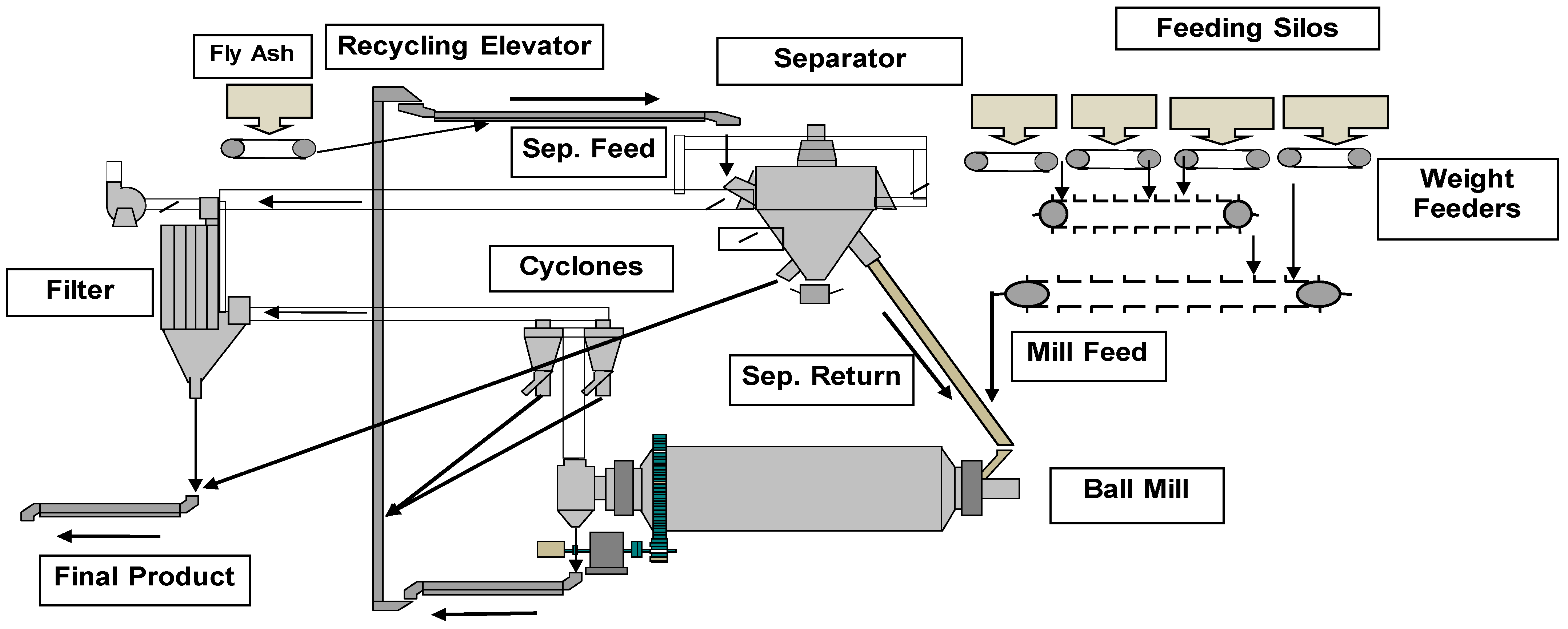
2. Process Description and Control Technique

2.1. Process Description and Materials Analysis

Cement plants typically grind cement in closed milling systems. Figure 1 shows a simplified flowchart of a grinding circuit, including all essential installations. We used the same configuration in [25] in a study of optimization of the process control of cement milling. The weight feeders feed the raw materials to either the ball mill or the separator (fly ash). The recycling elevator directs the output from the mill to the dynamic separator. The fine stream from the classifier constitutes the final product, whereas the coarse material returns to the CM for further grinding. The critical parameters related to quality include (i) cement fineness, (ii) separator speed, (iii) ratio of the coarse material-flow rate to the mill-feed rate, (iv) recycling elevator power, and (v) air-flow rate through the mill and pipes.

The plant quality department regulates the sulfates by sampling the cement in the mill outlet, measuring its SO₃ content, and adjusting the gypsum proportion in the CM feed. The control was applied to five CEM types produced according to EN 197-1:2011 [1] and is shown in

Table 1. CEM types.

CEM	Constituent (%) 1					28-Day Strength Limits (MPa)
	Clinker	Limestone (L)	Pozzolan (P)	Fly Ash (W)	Minor	Low	High
CEM I 52.5 N	95–100				0–5	52.5
CEM II A-L 42.5 N	80–94	<-- 6–20 -->			0–5	42.5	62.5
CEM II B-M (P-L) 32.5 N	65–79	<-------- 21–35 -------->			0–5	32.5	52.5
CEM IV B(P) 32.5 N-SR	45–64		<- 36–55 ->		0–5	32.5	52.5
CEM IV B(P-W) 32.5 N	45–64		<-------- 36–55 ------->		0–5	32.5	52.5

¹ Gypsum is not included in the composition but added according to SO₃ target.

. We presented the same Table in [19], where we optimized the sulfate content of the same CEM types. The range of the products is broad, covering Portland (I, II) and pozzolanic (IV) types as well as all three strength classes (32.5, 42.5, and 52.5).

Table 2. SO₃ of raw materials.

	Clinker	Limestone	Pozzolan	Fly Ash	Gypsum
Count	493	103	34	77	19
Average	0.93	0.02	0.0	2.49	42.78
Std. Dev.	0.33	0.02	0.0	1.43	2.88
%CV	35.5			44.8	6.7

presents the long-term statistics of the SO₃ content in the raw materials. The lab conducted analyses of Portland CEM types on Oxford Instruments (Oxfordshire, UK) LAB X 3000 (2005–2015) and Hitachi (Tokyo, Japan) X-Supreme 8000 (2016–2023) XRF analyzers, while Malvern-Panalytical (Almelo, The Netherlands) Axios-Cement and Zetium carried out the analyses of the raw materials and pozzolanic CEM types.

Both clinker and fly ash contain significant amounts of SO₃, with noticeable variations. The coefficient of variation %CV (=Std. Dev./Aver. × 100) lies within the range of 35.5% to 44.8%. The above causes two types of disturbance. (a) When the CEM type changes, the running composition can lead to a low-frequency step disturbance in the flow rate of sulfates due to differing percentages of clinker and (or) fly ash. Therefore, it is likely necessary to adjust the gypsum to achieve the current target. (b) The variation in SO₃ content of the two mentioned materials causes disturbances during operation with the same CEM type, necessitating attenuation by adjusting the proportion of gypsum.

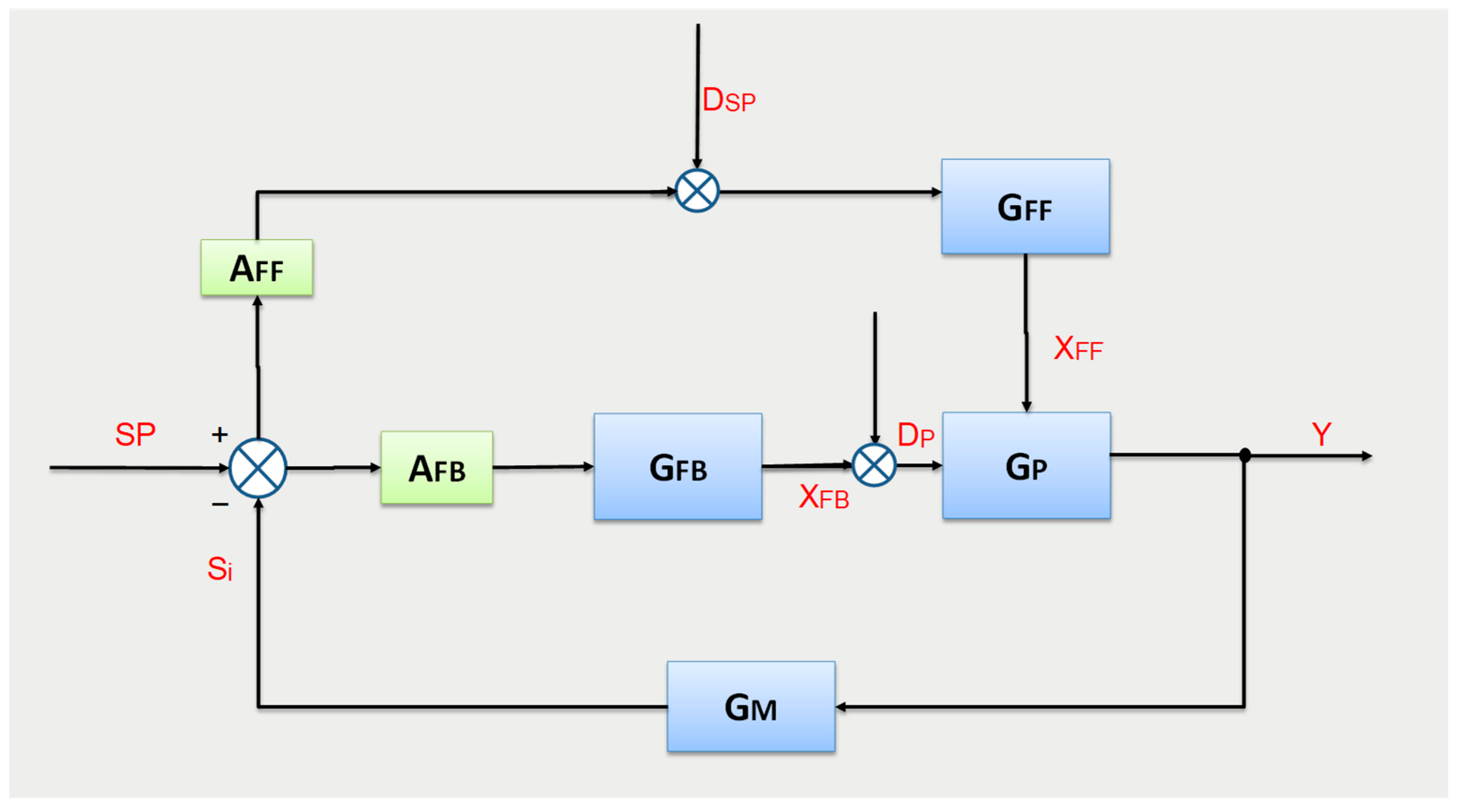
2.2. Controller Design

The presence of two distinct types of disturbances in the process variable provides the benefit of employing two controllers, acting separately on the control variable. Our earlier study introduced a dual regulator [21], comprising feedforward and feedback modules (FF–FB). Figure 2 depicts the block diagram of the transfer functions and signals related to the sulfate control.

The signal SP represents the SO₃ target of the current CEM, and D_SP is the signal for the SO₃ target in case the mill starts to grind another CEM type. D_SP is a low-frequency disturbance in the control loop that takes nonzero values only when there is a change in the cement type. X_FB and X_FF are signals expressing gypsum percentages derived from the FB and FF controllers. D_p is the SO₃ disturbance inserted into the process through the ingredient feeders (clinker, gypsum, and fly ash) due to the variance in the raw-materials composition. Signal Y represents the sulfate content of the product exiting the closed grinding circuit. S_i expresses the SO₃ percentage of the cement after sampling and measurement. Figure 2 shows the following transfer functions. G_P refers to the gypsum mixing within the milling system. G_M is a time delay function for sampling and sulfate measurement. G_FB and G_FF indicate the FB and FF controllers, respectively. If D_SP = 0, then A_FB = 1 and A_FF = 0. On the contrary, if D_SP ≠ 0, then A_FB = 0 and A_FF = 1.

Equations (2) and (3) provide, in the Laplace domain, the open loop transfer function G_OL and the transfer function from SP and disturbances to the output Y. G_OL represents the function of the system where the SO₃ output is not fed back to control the gypsum percentage.

$$G_{OL}=G_P·G_M·\left(A_{FB}·G_{FB}+A_{FF}·G_{FF}\right)$$

(2)

$$Y=\frac{G_P·\left(A_{FB}·G_{FB}+A_{FF}·G_{FF}\right)}{1+G_{OL}}·SP+\frac{G_P·G_{FF}}{1+G_{OL}}·D_{SP}+\frac{G_P}{1+G_{OL}}·D_P$$

(3)

Equation (4) expresses the G_M function. The average sampling and measuring time, T_M, which is a pure delay, is 0.25 h. As shown in reference [21], the transfer function G_P between the gypsum percentage in the CM feed and the %SO₃ in the final product can be modeled using first-order dynamics with time delay (FOTD). Equation (5) describes the model, where T_D is the delay time, T₀ is the time constant, and K_V is the gain.

$$G_M=e^{-T_M·s}$$

(4)

$$G_P=K_V·\frac{e^{-T_D·s}}{1+T_0·s}$$

(5)

According to [21], the milling circuit’s dynamic parameters are K_V = 0.4, T_D = 0.133 h, and T₀ = 0.233 h. The gain meaning is the increase in %SO₃ for a 1% increase in gypsum dosage. We conclude that the gain value is near the respective value computed from Table 2 (43.67/100 = 0.44). The meaning of T_D and T₀ is that after T_D, a step increase in gypsum will affect SO₃ in the CM outlet. After T₀, the SO₃ change is 63% of the total increase. Equation (6) provides the G_P transient response in the time domain after a ΔG step change in %gypsum.

$$\frac{S{O}_3\left(t\right)-S{O}_3\left(0\right)}{∆G}=K_V\left(1-e^{-\left(t-T_D\right)/T_0}\right)$$

(6)

SO₃(0) and SO₃(t) are the %SO₃ values at the beginning of the step increase and at time t, respectively. In the steady state, the maximum %SO₃ increase is ΔSO₃ = K_V·ΔG. Equation (7) computes the fraction a(t) of ΔSO₃ at time t.

$$a\left(t\right)=1-e^{-\left(t-T_D\right)/T_0}$$

(7)

Assuming that the system is near the steady state when the fraction α(t) reaches the value of 0.98, the required time calculated from Equation (7) is T_TP = 1.04 h. After this transient period, the system is in equilibrium with respect to step changes in gypsum feeding. For spot sampling, the delay time between the next and previous feedback controller outlets is the sum of T_TP and T_M, which is equal to T_s,Min = 1.29 h. T_s,Min is the minimum sampling period to avoid transient phenomena.

A simple integral controller (I) appropriately regulates the feedback control loop [21] with gain ki. Similarly, a proportional controller of gain K_FF attenuates the low-frequency disturbances of the feedforward loop. Equation (8) provides the respective transfer functions.

$$G_{FB}=\frac{k_i}{s} ; G_{FF}=K_{FF}$$

(8)

2.3. Digital Implementation

The feedback element of the controller calculates the gypsum setting of the CM feeder after each SO₃ measurement of an instantaneous (spot) sample, which is performed at regular time intervals. In contrast, the feedforward element acts only when the CM starts producing a different CEM type. Consequently, the controller operates in discrete time intervals characterized by the sampling period T_s. Equation (9) computes the error e_i between the SO₃ set point, S_SP, and the SO₃ of the sample taken at time i, S_i.

$$e_i=S_{SP}-S_i$$

(9)

The discrete implementation of the feedback integral controller utilizes the backward form [26] to calculate the gypsum percentage Gi at time i by adding the control action to the gypsum content Gi−1 of time i − 1. Equation (10) expresses this function. The sampling period is T_s = 2 h, and the optimal gain ki is 0.8, as found in an earlier simulation study [21]. The controller is unconstrained. The set of Equations (11)–(15) implements the feedforward proportional controller.

$$G_i=G_{i-1}+k_i·e_i·T_s$$

(10)

$$d_{SP}=\raisebox{1ex}{$\left[\left(C{l}_{CEM,N}-C{l}_{CEM,P}\right)·S_{Cl}+\left(As{h}_{CEM,N}-As{h}_{CEM,P}\right)·S_{Ash}\right]$}\!\left/ \!\raisebox{-1ex}{$100$}\right.$$

(11)

$$G_{Prev}=G_i ; S_P=S_i ; S_N=S_P+d_{SP} ; S_i=S_N$$

(12)

$$K_{FF}=\raisebox{1ex}{$100$}\!\left/ \!\raisebox{-1ex}{$S_G$}\right. ; DG=K_{FF}·\left(S_{SP}-S_i\right)$$

(13)

$$If ABS\left(DG\right)>Marg: if DG<0 :DG=-Marg elseif DG>0 DG=Marg$$

(14)

$$G_i=G_{Prev}+DG$$

(15)

S_P is the SO₃ measured at time i, G_Prev is the feedback controller output at time i, d_SP is the disturbance due to the CEM type change, and S_N is the SO₃ content considering the disturbance. Cl_CEM,P, Cl_CEM,N, Ash_CEM,P, and Ash_CEM,N are the average clinker and fly-ash contents of the previous and current CEM types, respectively. S_Cl, S_Ash, and S_G are the mean SO₃ contents of clinker, fly ash, and gypsum, as shown in Table 2. Equation (13) calculates the unconstrained output of the controller, DG. However, the optimal feedforward controller is constrained, as proven in [21]. The conditions in (14) implement the constraints for the maximum absolute change of the DG. Equation (16) calculates the value of the margin Marg, which depends on the previous and current CEM types.

$$Marg=ABS\left(\left(S_{SP,N}-S_{SP,P}-d_{SP}\right)·K_{FF}+M_0\right)$$

(16)

S_SP,P and S_SP,N are the SO₃ targets of the previous and current CEM, respectively, and M₀ is an additional margin of gypsum. In our application, M₀ = 0.5.

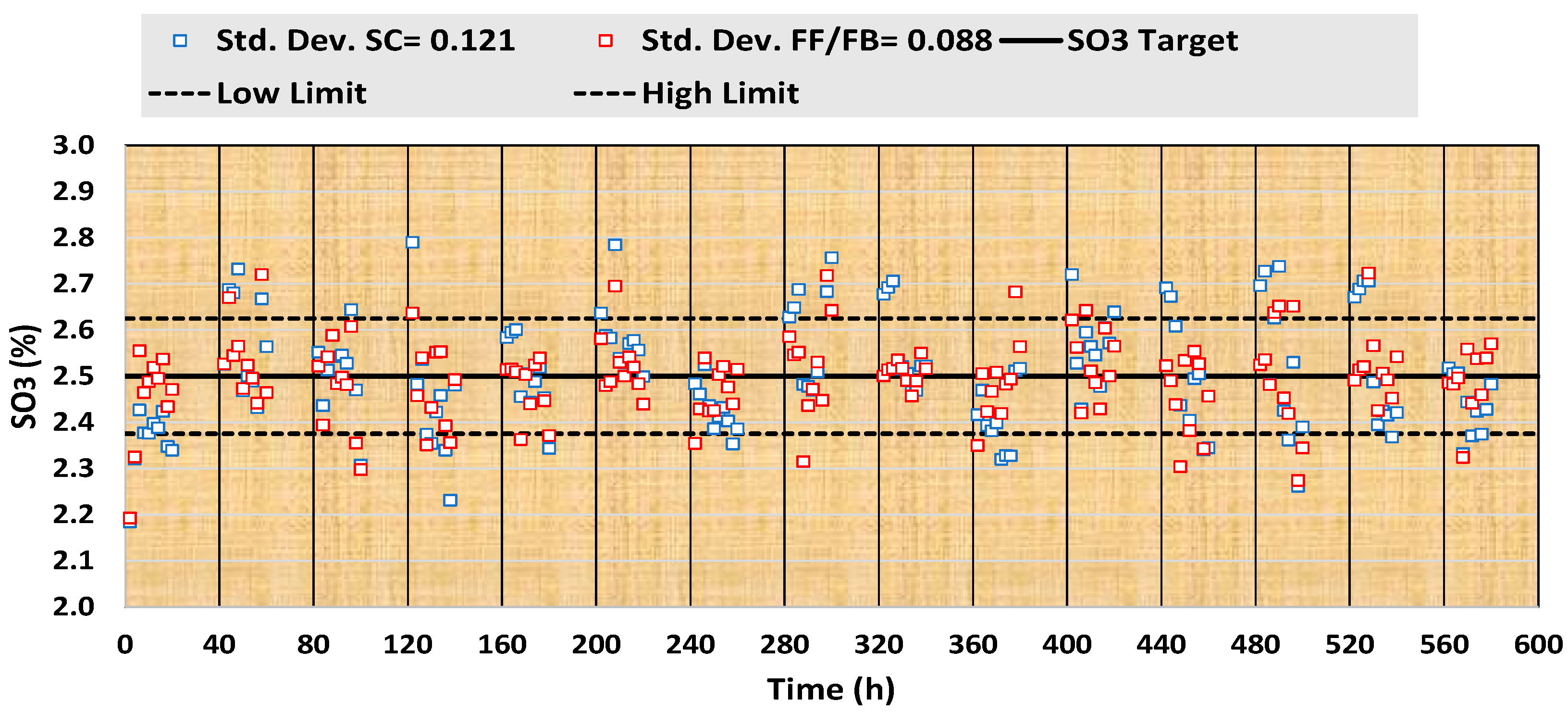
2.4. Comparisons Using a Process Simulator

For the past eleven years, the FF–FB controller designed in Section 2.2 has been operating in CM5 and CM6 of the Halyps plant to regulate the sulfates for all the CEM types produced. Before using this regulator, the plant employed the step rules (SC) controller, as mentioned in [21] and shown in Equation (17). This regulator consists of a dead band of 0.4 for SO₃ and provides step changes in the gypsum feed with a gain of 0.5 or a multiple thereof. The description of Equations (11)–(15) provides the physical meaning of the parameters of Equation (17).

$$\begin{gathered} e_i ϵ \left[-0.2 , 0.2\right] \to DG=0 \\ {e}_i ϵ \left[0.2 , 0.6\right] \to DG=0.5 \\ {e}_i ϵ \left[0.6 , 1.0\right] \to DG=1.0 \\ {e}_i>1.0 \to DG=1.5 \\ {e}_i ϵ \left[-0.6 ,-0.2\right] \to DG=-0.5 \\ {e}_i ϵ \left[-1.0 ,-0.6\right] \to DG=-1.0 \\ {e}_i<-1.0 \to DG=-1.5 \\ {G}_i=G_{i-1}+DG \end{gathered}$$

(17)

Process simulators allow comparisons between SC and FF–FB controllers. The simulator runs the CM for 600 h. The cement type changes every 20 h between CEM II B-M (P-L) 32.5 and CEM II A-L 42.5. A disturbance occurs in clinker SO₃ every 10 h, i.e., two disturbances appear every 20 h. Clinker SO₃ never changes when the CEM type changes. The simulator creates the magnitude of each disturbance using a predefined mean and standard deviation of clinker SO₃, a randomly generated probability, and the inverse normal distribution. The simulator also calculates a low variation in gypsum sulfate every 2 h.

Table 3. Simulator parameters.

	CEM II B-M (P-L) 32.5	CEM II A-L 42.5
SO3 target (%)	2.5	3
Clinker content (%)	65	80
SO3 low limit (%) (=0.95 of SO3 target)	2.375	2.85
SO3 high limit (%) (=1.05 of SO3 target)	2.625	3.15
Initial gypsum (%)	4.0
Initial SO3 (%)	2.80
Sampling period (h)	2.0
Clinker mean SO3 (%)	0.93
Clinker SO3 standard deviation (%)	0.20
Gypsum mean SO3 (%)	42.78
Gypsum SO3 standard deviation (%)	1.0

lists the parameters of the developed simulation. Figure 3 shows the SO₃ results for the SC and FF–FB controllers for the CEM II B-M (P-L) 32.5. The simulator used the same disturbances for both control techniques. Compared to SC, the FF–FB results have less dispersion around the target.

A quantitative comparison of the two controllers’ performances is feasible by implementing the simulator multiple times. The simulator used the same disturbances for each run.

Table 4. Statistical results of simulator application.

CEM	II B-M (P-L) 32.5			II A-L 42.5
	SC	FF–FB	Ratio	SC	FF–FB	Ratio
Standard deviation, sSC, sFF/FB (%)	0.134	0.109		0.146	0.125
sFF/FB/sSC			0.812			0.854
(%) of population out of [0.95·SSP, 1.05·SSP] PSC, PFF/FB	32.1	15.4		27.3	14.6
PFF/FB/PSC			0.481			0.534
(%) of population out of [0.95·SSP, 1.05·SSP] in CEM type change, CSC, CFF/FB	38.1	9.6		36.5	5.6
CFF/FB/CSC			0.251			0.154

presents the average statistical results after 100 implementations.

We used three criteria to evaluate the closeness to S_SP: (a) the average standard deviation, (b) the percentage of the population out of the interval [0.95·S_SP, 1.05·S_SP], and (c) the same statistic as (b) but for the first SO₃ values when the CEM type changes. Criterion (c) assesses the efficiency in set-point tracking, whereas criteria (a) and (b) evaluate the degree of disturbance rejection. The three statistics’ ratios are consistently smaller than one, indicating that the FF–FB system outperforms the SC in disturbance attenuation and set-point tracking.

3. Long-Term Results and Analysis

3.1. Shewhart Control Charts and Nonparametric Analysis

The Shewhart control charts [27] (pp. 8–9) are suitable for comparing the results of the two control techniques in the long term. These charts require data in rational subgroups taken at approximately regular intervals during the process. In this study, each subgroup contains all the SO₃ results of samples taken during one year per CM and CEM type. We performed the comparison by generating mean ($\overline{X}$) and standard deviation (s) charts. We separated the results into two groups: (a) the period of SO₃ adjustment using Equation (16) (2005–2012) and (b) the period of FF–FB controller application (2013–2023). The central line (CL) of the $\overline{X}$-chart is a prespecified process parameter equal to the SO₃ target per CEM type. Because the number of samples n_i varies annually, we used the pooled standard deviation s_Pk [28] (p. 93) to determine the central line of the s-chart and the control limits, as shown in Equation (18).

$$s_{Pk}={\left(\frac{{\sum }_{i=1}^M\left(n_{ik}-1\right)·s_{ik}^2}{{\sum }_{i=1}^{Mk}{n}_{ik}-M_k}\right)}^{\raisebox{1ex}{$1$}\!\left/ \!\raisebox{-1ex}{$2$}\right.} i=1,2\dots M_k k=1: SC and k=2:FF/FB$$

(18)

where M_k is the number of years in the selected period and s_ik is the SO₃ standard deviation of year i and period k. The annual number of samples is sufficient to calculate statistics when n_ik ≥ 20.

There is a maximum size of 25 samples in each subgroup in Table 2 of ISO 7870-2 [27] (p. 9), which includes the factors to compute the lower and upper control limits, L_CL and $U_{CL}$. This table is not suitable because all n_ik exceed this value. Reference [29] provides the general formulae to determine the control limits L_CL and $U_{CL}$, applicable to any number N of samples and given by Equations (19)–(21).

$$\overline{X}-chart: L_{CL}=CL-3·\raisebox{1ex}{$s_{Pk}$}\!\left/ \!\raisebox{-1ex}{$c_4\sqrt{N}$}\right. U_{CL}=CL+3·\raisebox{1ex}{$s_{Pk}$}\!\left/ \!\raisebox{-1ex}{$c_4\sqrt{N}$}\right.$$

(19)

$$s-chart: L_{CL}=s_{Pk}-3·s_{Pk}·\raisebox{1ex}{$\sqrt{1-c_4^2}$}\!\left/ \!\raisebox{-1ex}{$c_4$}\right. U_{CL}=s_{Pk}+3·s_{Pk}·\raisebox{1ex}{$\sqrt{1-c_4^2}$}\!\left/ \!\raisebox{-1ex}{$c_4$}\right.$$

(20)

$$c_4=\sqrt{\frac{2}{N-1}}·\frac{\left(\raisebox{1ex}{$N$}\!\left/ \!\raisebox{-1ex}{$2$}\right.-1\right)!}{\left(\raisebox{1ex}{$\left(N-1\right)$}\!\left/ \!\raisebox{-1ex}{$2$}\right.-1\right)!}$$

(21)

where the coefficient c₄ uses the noninteger factorial, determined by the Gamma function and its properties: Γ(x + 1) = x·Γ(x) and Γ(½) = π^1/2.

Figure 4, Figure 5, Figure 6, Figure 7 and Figure 8 illustrate the two kinds of control charts for the CEM types produced in both periods under examination. For each period, the number N needed for determining the upper and lower control limits is the average of the populations of yearly samples.

The mean charts depict the closeness of the annual mean SO₃ to the target. In all CEM types and both CMs, applying the FF–FB controller leads these two variables into proximity. In the case of the SC regulator, the average sulfates and their target are close for the Portland types but not for the pozzolanic cement. The comparison of the differences between the target, ST_ik, and the realized SO₃, Sav_ik, requires a statistical test. Equation (22) computes the absolute value d_ik of this difference, and Figure 9a,b shows this function for two CEM types.

$$d_{ik}=\left|S{T}_{ik}-Sa{v}_{ik}\right| i=1..M_k and k=1,2$$

(22)

Due to the asymmetry of all distributions, statistical tests based on the normal distribution are not applicable. Therefore, estimating the difference of means ([30], pp. 18–19) is inapplicable, and the test shall be nonparametric. Mann and Whitney [31] developed such a statistic, which the relative literature [32,33,34] continuously refers to, finding implementation in several research fields [35,36,37,38]. This test concerns the sets D₁ and D₂ with populations M₁ and M₂ described in (23).

$$D_1=\left\{d_{11},d_{21},\dots d_{M_{1}1}\right\} D_1=\left\{d_{12},d_{22},\dots d_{M_{2}2}\right\}$$

(23)

The method considers the set D = D₁∪D₂ and finds the rank of each element within the union D after sorting them in increasing order. R₁ and R₂ are the sum of the ranks for observations one and two. Equation (24) provides the test statistic $U$, which shall be compared with the critical values $U_{cr}$.

$$\begin{array}{l}{U}_1=M_1{M}_2+\frac{M_1\left(M_1+1\right)}{2}-R_1 U_2=M_1{M}_2+\frac{M_2\left(M_2+1\right)}{2}-R_2 U\\ \hspace{1em}\hspace{1em}\hspace{1em}\hspace{1em}\hspace{1em}\hspace{1em}\hspace{1em}\hspace{1em}=\min \left(U_1, U_2\right)\end{array}$$

(24)

The null hypothesis H₀ is that there is no tendency for the ranks of D₁ to be significantly higher than that of D₂ occurring when $U>U_{cr}$. The alternative hypothesis H_A is that the ranks of D₁ are systematically higher than that of D₂ occurring when $U\le U_{cr}$. The hypotheses show that the test is one tail, and reference [39] provides the critical values for probabilities a = 0.01 and a = 0.05.

Table 5. Mann–Whitney test for the sets D₁ and D₂.

	CEM II B-M (P-L) 32.5	CEM II A-L 42.5	CEM IV B (P-W) 32.5
M1	16	15	6
M2	21	14	10
$U$	140	62	3
$U_{cr}$ for a = 0.01	92	51	8
$U_{cr}$ for a = 0.05	113	66	14

presents the results of the Mann–Whitney test for sets D₁ and D₂, leading to the following conclusions. The two controllers have equivalent performance concerning the CEM II B-M (P-L) 32.5. On the contrary, in CEM II A-L 42.5, the annual mean values better approximate the target using the FF–FB controller than applying the SC, with a probability of 95%. This improvement is most noticeable at CEM B (P-W) 32.5, where the values of the D₁ set are higher than those of D₂ with a probability of 99%.

The s-charts shown in Figure 4b, Figure 5b, Figure 6b, Figure 7b and Figure 8b illustrate a pronounced decrease in the annual standard deviation after the FF–FB controller started operating. The $U_{CL}$ of FF–FB is always lower than the L_CL of SC, indicating that the former controller attenuates disturbances caused by sulfate variability in the raw materials better than the latter.

Table 6. Pooled standard deviations.

CEM	II B-M (P-L) 32.5	II A-L 42.5	IV B (P-W) 32.5	I 52.5	IV B (P) 32.5
CM5 sP1	0.145	0.142	0.241
CM5 sP2	0.086	0.083	0.095	0.126	0.096
CM5 sP2/sP1	0.59	0.58	0.39
CM6 sP1	0.151	0.134
CM6 sP2	0.078	0.072
CM6 sP2/sP1	0.51	0.53

shows the pooled standard deviations for the five CEM types produced and their ratios when a CEM covers both periods (SC and FF–FB).

The severe and systematic improvement of SO₃ stability using the FF–FB controller is apparent in this table. The ratio of s_P2–s_P1 ranges from 0.51 to 0.59 for Portland CEM types, where the regulating action is the attenuation of clinker variability in SO₃. The improvement is better in pozzolanic cement CEM IV B (P-W) 32.5, where SO₃ disturbances originate from fly ash and clinker. The two pozzolanic types show similar standard deviations. Despite its high clinker content, CEM I 52.5 shows a lower pooled standard deviation during FF–FB operation than the respective values of all CEM types during SC operation.

3.2. Assessing Controllers’ Quality by Combining Standard Uncertainties

Cement SO₃ is the sum of the sulfates in the clinker, fly ash, and gypsum. Consequently, accounting for error propagation, the variance and covariance of input variables affect cement SO₃ variability. We assume that between an output y and input variables, there is a functional relationship y = f(x₁, x₂, … x_N). Then, Equation (25) provides the square of the combined standard uncertainty $u_c^2\left(y\right)$ as a function of the uncertainties u(x_i) [28] (pp. 18–23).

$$u_c^2\left(y\right)={\displaystyle \sum }_{i=1}^N{\left(\frac{\partial f}{\partial x_i}\right)}^2·u^2\left(x_i\right)+2·{\displaystyle \sum }_{i=1}^{N-1}{\displaystyle \sum }_{j=i+1}^{N}r\left(i,j\right)·\frac{\partial f}{\partial x_i}·\frac{\partial f}{\partial x_j}·u\left(x_i\right)·u\left(x_j\right)$$

(25)

where r(i, j) is the correlation coefficient between x_i and x_j. r(i, j) = 0 for uncorrelated variables, and it is positive or negative for positively or negatively correlated variables.

Equation (26) illustrates the sulfate mass balance of cement, where CL, G, and FA denote the fractions of clinker, gypsum, and fly ash in the cement composition, S_CL, S_G, and S_FA are the sulfates coming from the raw materials, and SO_3,CEM, SO_3,CL, SO_3,G, and SO_3,FA are the SO₃ percentages in cement and in the three materials.

$$S{O}_{3,CEM}=S_{CL}+S_G+S_{FA} S_{CL}=CL·S{O}_{3,CL} S_G=G·S{O}_{3,G} S_{FA}=FA·S{O}_{3,FA}$$

(26)

The pairs of variables (CL, SO_3,CL), (G, SO_3,G), and (FA, SO_3,FA) are uncorrelated. Therefore, Equations (27)–(29) give the uncertainties u_S,CL, u_S,G, and u_S,FA of SO₃ of each component within the CEM composition.

$$u_{S,CL}^2=C{L}^2·u_{SO3,CL}^2+u_{CL}^2·S{O}_{3,CL}^2$$

(27)

$$u_{S,G}^2=G^2·u_{SO3,G}^2+u_G^2·S{O}_{3,G}^2$$

(28)

$$u_{S,FA}^2=F{A}^2·u_{SO3,FA}^2+u_{FA}^2·S{O}_{3,FA}^2$$

(29)

where u_CL, u_G, u_FA are the uncertainties of the fractions CL, G, and FA in the CM feeders, SO_3,CL, SO_3,G, SO_3,FA are the sulfates of CL, G, and FA, and u_SO3,CL, u_SO3,G, u_SO3,FA are the respective uncertainties. If a controller regulates cement SO₃ by changing the gypsum, the variables S_CL and S_G are negatively correlated. The same occurs for S_FA and S_G. Equation (30) specifies this case for the uncertainty of cement sulfates u_S,CEM.

$$u_{S,CEM}^2=u_{S, CL}^2+u_{S,G}^2+u_{S,FA}^2-2r\left(CL,G\right)·u_{S,CL}·u_{S,G}-2r\left(FA,G\right)·u_{S,FA}·u_{S,G}$$

(30)

where the correlation coefficients of CL and G, r(CL, G), and of FA and G, r(FA, G) belong to the interval [0, 1]. The model of Equations (26)–(30) requires the estimation of correlation coefficients based on actual quality data of each CEM type and raw material.

Table 7. Variables of error propagation model and type of quality data.

Variable	Type of Quality Data
uS,CEM	Annual standard deviation of the SO3 daily data
CL, G, FA	Annual average of clinker, gypsum, and fly-ash fractions in CEM composition calculated from daily data chemical analysis
uCL, uG, uFA	Annual standard deviation of clinker, gypsum, and fly-ash fractions in CEM composition calculated from daily data chemical analysis
SO3,CL, uSO3,CL	Annual average and standard deviation of clinker SO3 calculated from daily data
SO3,G, uSO3,G, SO3,FA, uSO3,FA	Annual average and standard deviation of gypsum and fly-ash SO3 calculated from the samples taken in one year

demonstrates the type of data used for all the variables.

In the case of cement containing up to four components (clinker, gypsum, limestone, and pozzolan), we determined the daily fractions of clinker and gypsum in the composition by using SO₃, loss on ignition, and insoluble residue [40] of cement and raw materials and solving the respective linear system. In the case of cement with fly ash (CEM IV B (P-V) 32.5), we also utilized the oxides CaO, SiO₂, and Al₂O₃ to estimate the fly-ash content using the generalized reduced gradient nonlinear regression technique. We applied the same nonlinear method to calculate the correlation coefficients. A strong relationship exists between these coefficients and the ability of a controller to reject or attenuate disturbances. The larger the correlation coefficient between gypsum and clinker or fly ash, the more robustly the regulator adjusts the gypsum percentage to compensate for clinker or fly-ash sulfate disturbances or changes in cement composition.

Table 8. Regression results analysis of the standard deviation results.

Controller	Count	r(CL, G)	r(FA, G)	Standard Error	Standard Deviation	R2
SC	37	0.876	0.006	0.01359	0.03542	0.853
FF–FB	50	0.962	0.647	0.00833	0.03988	0.956

shows the regression analysis of the standard deviation results after each controller was applied. We provide Table S1 with all the lab data used in the error propagation analysis for the two applied control techniques and all CEM types.

The correlation coefficient between clinker and gypsum, r(CL, G), using the FF–FB is significantly higher than that using the SC controller. The above perfectly explains the considerable improvement in the annual standard deviation in Portland cement, shown in Table 8. Applying the SC controller, the r(FA, G) is around null, becoming significant using the FF–FB. The conclusion is that FA and G are uncorrelated, and the SC cannot compensate for SO₃ disturbances in fly ash, which the FF–FB controller satisfactorily achieves, resulting in a noticeable drop in the pooled standard deviation for the pozzolanic cement. Figure 10a,b compares actual and calculated values, y_act and y_calc, whereas Equations (31) and (32) provide these two variables. This figure clearly explains the significant increase in R² in the FF–FB case compared with the R² of SC.

$$y_{act}=u_{s,CEM}^2-u_{s, CL}^2-u_{s,G}^2-u_{s,FA}^2$$

(31)

$$y_{calc}=-2r\left(CL,G\right)·u_{s,CL}·u_{s,G}-2r\left(FA,G\right)·u_{s,FA}·u_{s,G}$$

(32)

4. Conclusions

This study analyzes the design of a feedforward and feedback mechanism and its implementation in an industrial control system for cement sulfates. The controller considers all the fundamental aspects and particularities of the grinding process and quality requirements. (a) Variability of the raw materials SO₃; (b) CM dynamics; (c) sampling period and measuring delays; (d) cement composition and feeders’ accuracy; and (e) grinding of various CEM types with different sulfate targets. The results of the FF–FB controller, long-term applied in two CMs of the Halyps plant for all CEM types, have been compared with those of the previously applied controller, which used step rules to adjust gypsum. The main conclusions of this study are as follows.

(1)

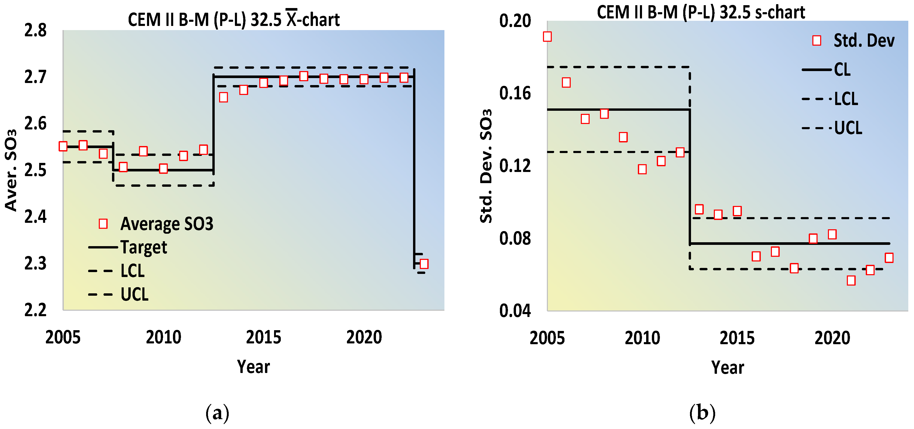
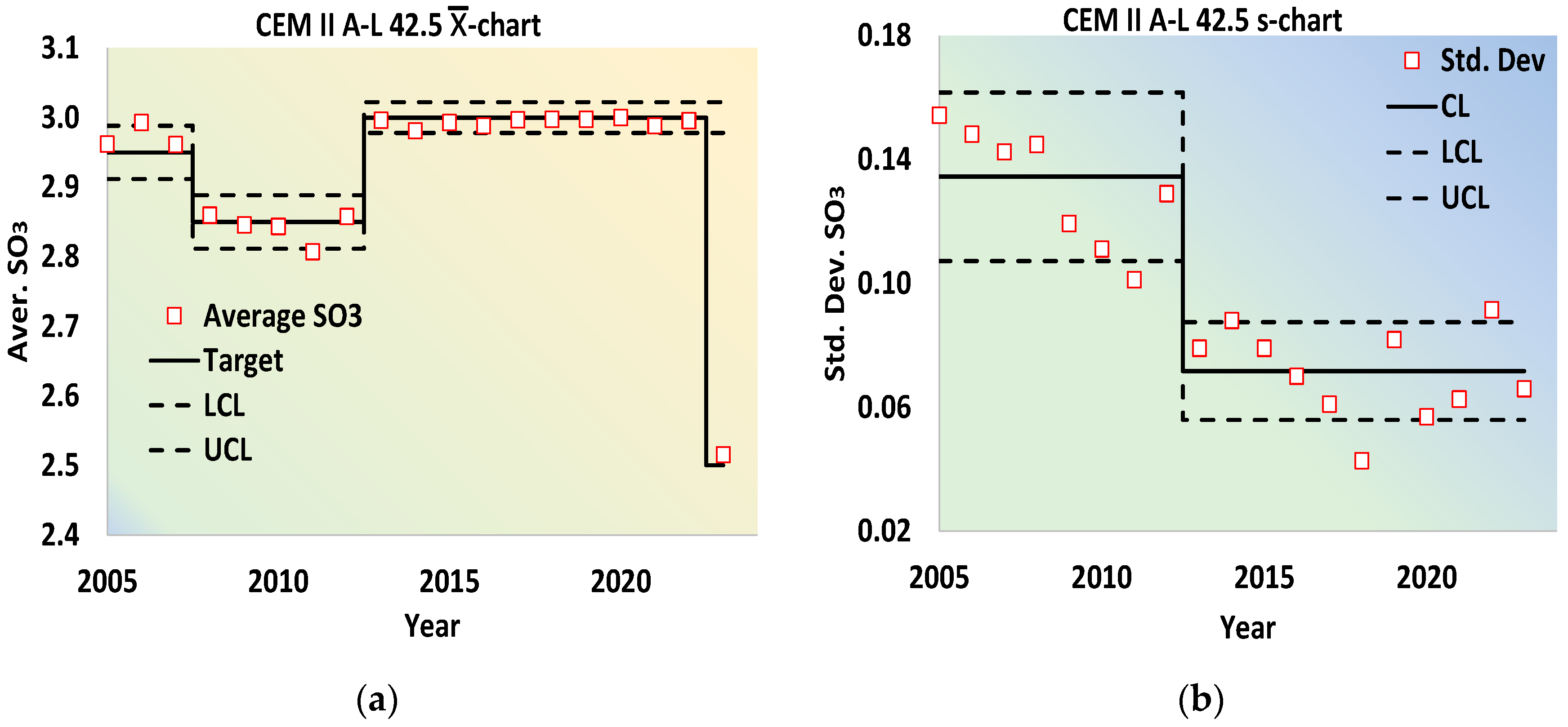
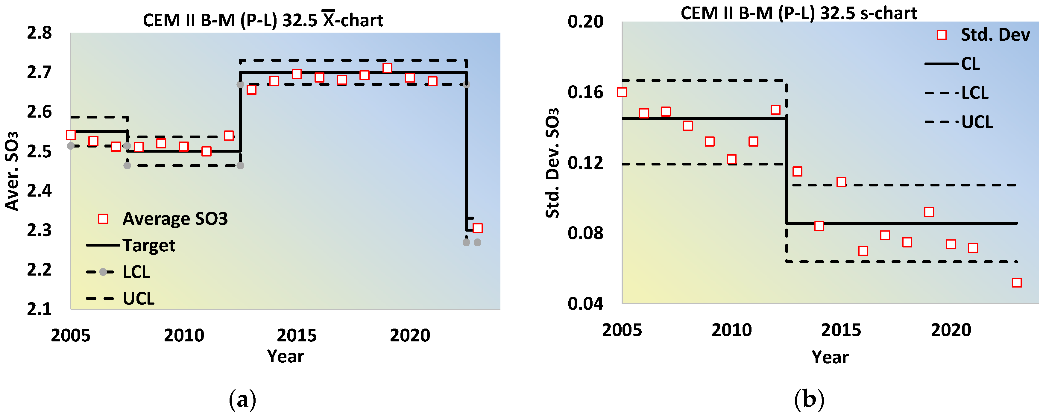
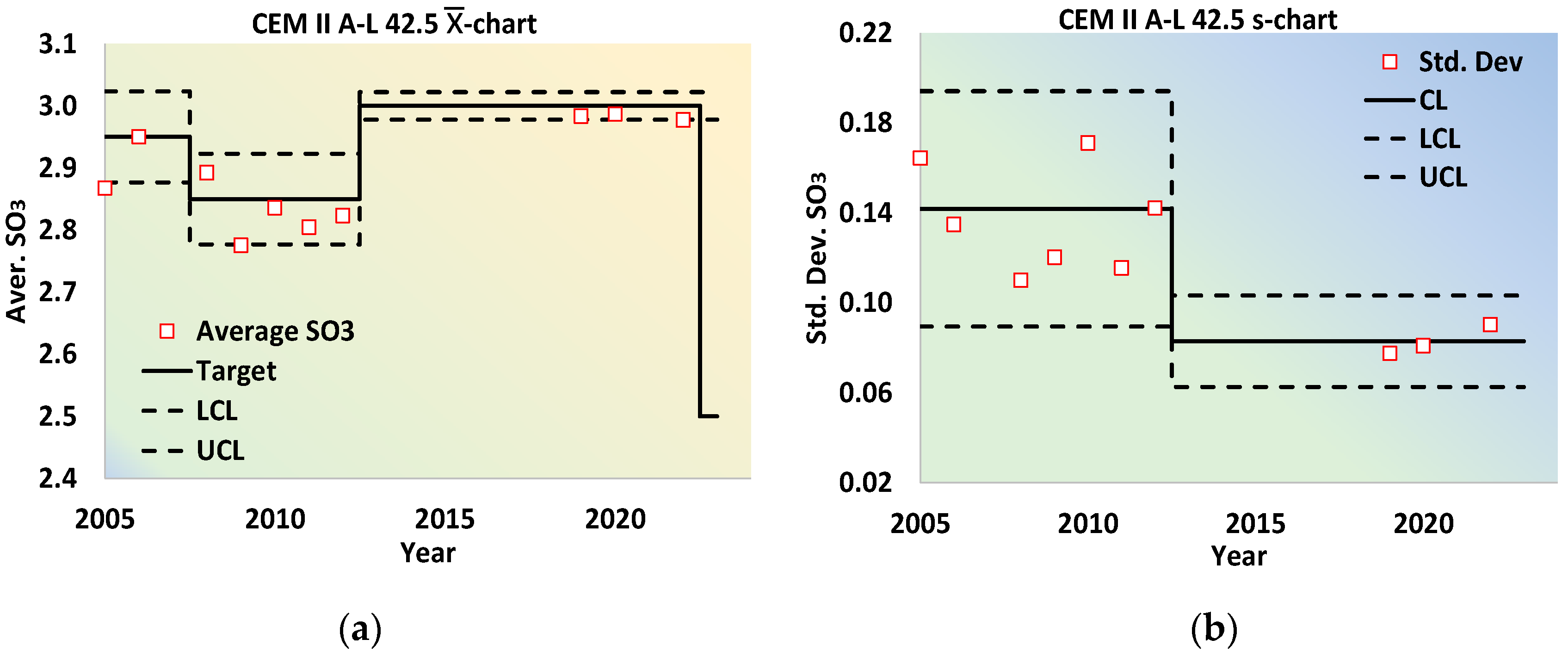
The Shewhart $\overline{X}$-charts of the annual SO₃ mean values and the nonparametric Mann–Whitney statistical test prove that using the FF–FB controller, the mean values approach better the SO₃ target than the SC controller in two out of the three CEM types produced continuously for eighteen years;

(2)

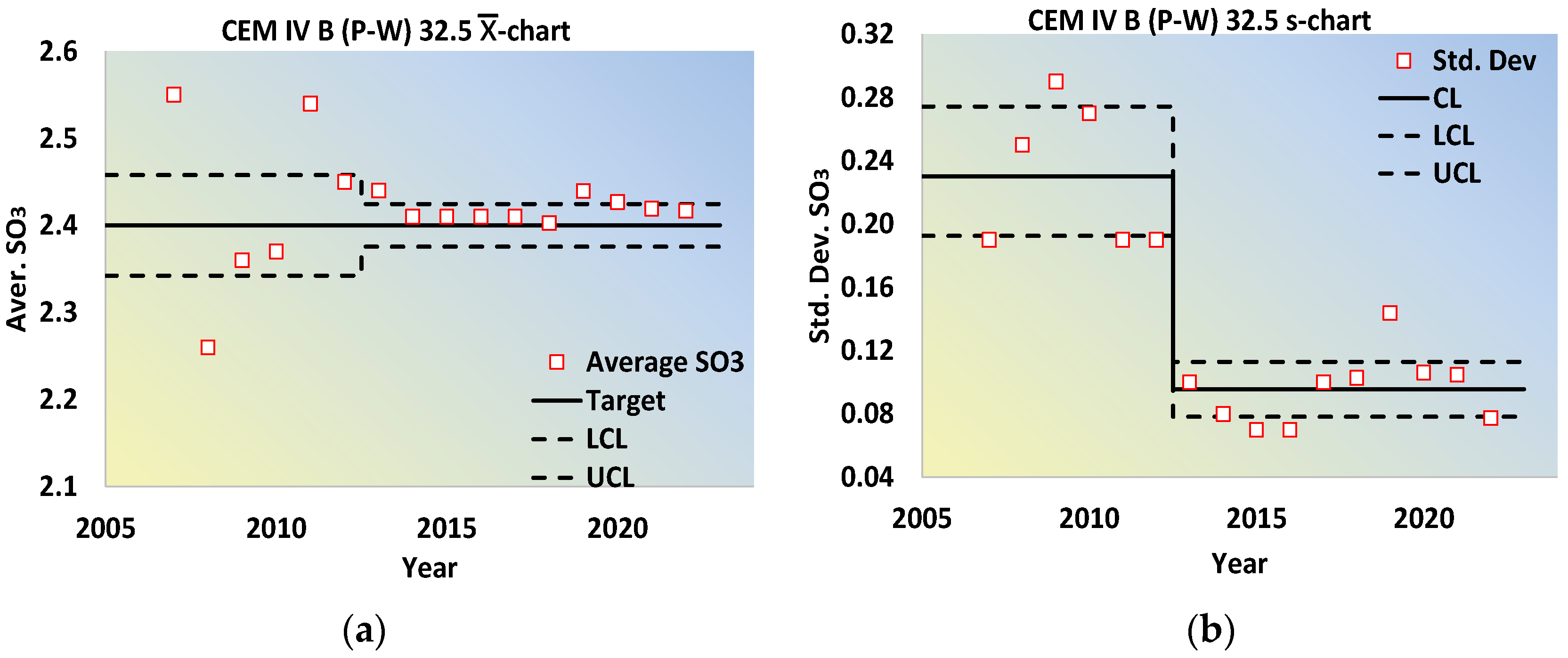
FF–FB is better than SC in target approximation with a probability of 95% (a = 0.05) in CEM II A-L 42.5. The two controllers do not show distinguishable performance for the same test level a in CEM II B-M 32.5. This resulted from the second CEM type reduced clinker content and the consequent milder variance of clinker SO₃ within the cement composition. In contrast, the ability of FF–FB to regulate gypsum is better than SC so the SO₃ values are closer to the target and appear in CEM II A-L 42.5. Compared with CEM II B-M 32.5, this cement has a higher clinker content, which causes a higher variation in SO₃ within the composition. The enhanced performance of FF–FB is more distinct in the pozzolanic cement, where clinker and fly ash are the two independent sources of sulfate disturbances because the test rejects the null hypothesis of equivalence with a probability of 99%;

(3)

The Shewhart s-charts of the annual standard deviation per CEM type and CM show that the FF–FB controller performs substantially better than the SC. The $U_{CL}$ of the former is always lower than the L_CL of the latter. The ratio of the central lines of FF–FB to SC ranges from 0.51 to 0.59 for the Portland CEM types. This ratio is further reduced to 0.39 in pozzolanic cement CEM IV B (P-W) 32.5, where SO₃ disturbances originate from fly ash and clinker;

(4)

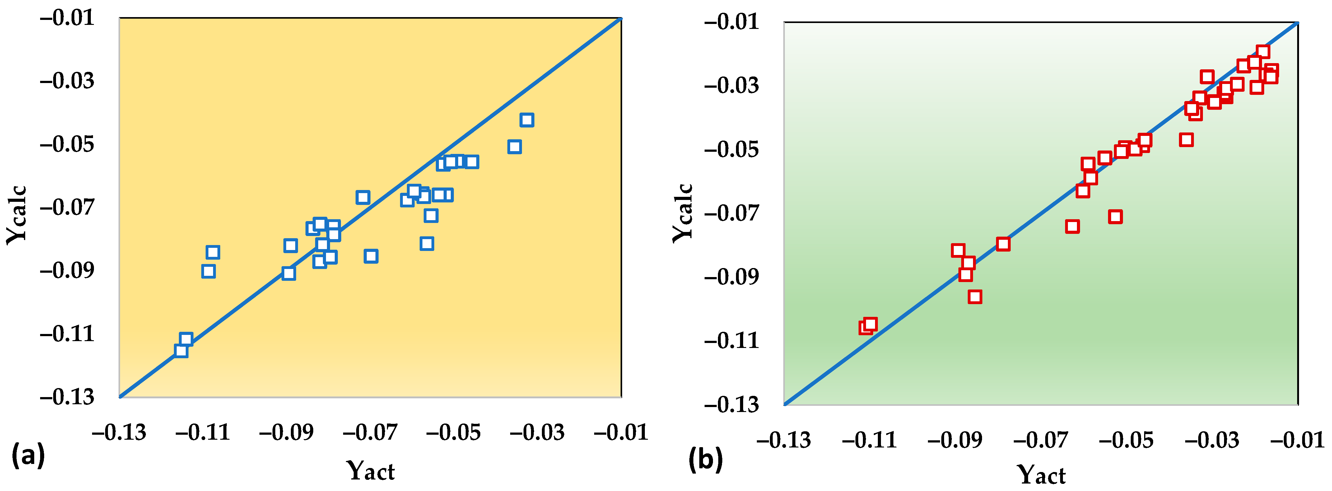
Our analysis illustrates that the error propagation method is appropriate for comparing controller performance. If a controller regulates the cement sulfates by changing the gypsum, the SO₃ contained in the gypsum and clinker are negatively correlated. The same occurs for SO₃ in gypsum and fly ash. The larger the absolute value of correlation coefficients, the more robustly the controller regulates the gypsum content to compensate for clinker or fly-ash sulfate disturbances or changes in cement composition. The coefficients r(CL, G) and r(FA, G) are 0.876 and 0.006, respectively, using the SC controller. In the FF–FB case, the values are essentially higher, 0.962 and 0.647, respectively. The above clearly explains the higher performance of the feedforward–feedback system compared with SC.

To the best of the author’s knowledge, it is hard to find a description of cement sulfate controllers installed in milling systems in the literature. The technical novelty of this research is the design and long-term industrial implementation of such a system comprising a feedforward and feedback component. The FF component tracks the set-point changes of SO₃ when the cement mill starts to grind another CEM type, and the FB controller effectively attenuates the variations of the raw materials’ sulfates.

Cement factories today use various alternative fuels to reduce their carbon footprint per clinker ton. Their highly changeable mix composition and sulfur level increase the SO₃ variance of clinker, making it indispensable to implement an optimized controller to regulate sulfates around the target. An optimal SO₃ target provides the maximum compressive strength [19] and permits clinker reduction in cement composition, further contributing to the decrease in CO₂ per ton of product. Consequently, the actions to optimize and regulate SO₃ are interconnected, resulting in a positive environmental impact.

We selected spot cement sampling and a sampling period such that transient dynamic phenomena are negligible. Further development of the research on optimal controllers regulating SO₃ in the CM outlet involves designing a control system where the sampling is continuous, providing an average sample for each T_s period. This type of controller must account for the transient phenomena that occur during the mean sample preparation.

References

- EN 197-1:2011; Cement—Part 1: Composition, Specifications and Conformity Criteria for common Cements. CEN/TC 51; CEN: Brussels, Belgium, 2011; pp. 10–15.
- C150/C150M-22; Standard Specification for Portland Cement. ASTM International: West Conshohocken, PA, USA, 2022.
- Mindess, S.; Young, J.F.; Darwin, D. Concrete, 2nd ed.; Prentice Hall: Upper Saddle River, NJ, USA, 2003; Volume 31, pp. 60–62. [Google Scholar]
- Niemuth, M. Effect of Fly Ash on the Optimum Sulfate of Portland Cement. Ph.D. Dissertation, Purdue University, West Lafayette, IN, USA, December 2012; p. 68. Available online: https://www.researchgate.net/publication/266077758_Effect_of_Fly_Ash_on_Optimum_Sulfate_of_Portland_Cement (accessed on 23 November 2023).
- Evans, K.A. The Optimum Sulphate Content in Portland Cement. p. 3. Available online: https://tspace.library.utoronto.ca/bitstream/1807/11621/1/MQ29389.pdf (accessed on 7 April 2023).
- Lerch, W. The Influence of Gypsum on the Hydration and Properties of Portland Cement Pastes. In Proceedings of the American Society for Testing Materials; American Concrete Institute (ACI): Farmington Hills, MI, USA, 1946; Volume 46, pp. 1252–1291. [Google Scholar]
- Bentur, A. Effect of Gypsum on the Hydration and Strength of C3S Pastes. J. Am. Ceram. Soc. 1976, 59, 210–213. [Google Scholar] [CrossRef]
- Soroka, I.; Abayneh, M. Effect of gypsum on properties and internal structure of PC paste. Cem. Concr. Res. 1986, 16, 495–504. [Google Scholar] [CrossRef]
- Sersale, R.; Cioffi, R.; Frigione, G.; Zenone, F. Relationship between gypsum content, porosity and strength in cement. I. Effect of SO3 on the physical microstructure of Portland cement mortars. Cem. Concr. Res. 1991, 21, 120–126. [Google Scholar] [CrossRef]
- Gunay, S.A.A. Influence of Aluminates Phases Hydration in Presence of Calcium Sulfate on Silicates Phases Hydration: Consequences on Cement Optimum Sulfate. Ph.D. Thesis, University of Bourgogne, Bourgogne, France, 2012. Available online: https://theses.hal.science/tel-00767768 (accessed on 7 April 2023).
- Zunino, F.; Scrivener, K. The influence of sulfate addition on hydration kinetics and C-S-H morphology of C3S and C3S/C3A systems. Cem. Concr. Res. 2022, 160, 106930. [Google Scholar] [CrossRef]
- Andrade Neto, J.S.; de Matos, P.R.; De la Torre, A.G.; Campos, C.E.M.; Torres, S.M.; Monteiro, P.J.M.; Kirchheim, A.P. Hydration and interactions between pure and doped C3S and C3A in the presence of different calcium sulfates. Cem. Concr. Res. 2022, 159, 106893. [Google Scholar] [CrossRef]
- Mohammed, S.; Safiullah, O. Optimization of the SO3 content of an Algerian Portland cement: Study on the effect of various amounts of gypsum on cement properties. Constr. Build. Mater. 2018, 164, 262–370. [Google Scholar] [CrossRef]
- Adu-Amankwah, S.; Black, L.; Skocek, J.; Ben Haha, M.; Zajac, M. Effect of sulfate additions on hydration and performance of ternary slag-limestone composite cements. Constr. Build. Mater. 2018, 164, 451–462. [Google Scholar] [CrossRef]
- Han, F.; Zhou, Y.; Zhang, Z. Effect of gypsum on the properties of composite binder containing high- volume slag and iron tailing powder. Constr. Build. Mater. 2020, 252, 119023. [Google Scholar] [CrossRef]
- Yamashita, H.; Yamada, K.; Hirao, H.; Hoshino, S. Influence of Limestone Powder on the Optimum Gypsum Content for Portland Cement with Different Alumina Content. Available online: https://www.researchgate.net/publication/285554157_Influence_of_Limestone_Powder_on_the_Optimum_Gypsum_Content_for_Portland_Cement_with_Different_Alumina_Content (accessed on 23 November 2023).
- Liu, F.; Lan, M.Z. Effects of Gypsum on Cementitious Systems with Different Mineral Mixtures. Available online: https://www.researchgate.net/publication/269647645_Effects_of_Gypsum_on_Cementitious_Systems_with_Different_Mineral_Mixtures (accessed on 23 November 2023).
- Fincan, M. Sulfate Optimization in the Cement-Slag Blended System Based on Calorimetry and Strength Studies. Ph.D. Thesis, University of South Florida, Tampa, FL, USA, 2021; p. 2. Available online: https://digitalcommons.usf.edu/cgi/viewcontent.cgi?article=9967&context=etd (accessed on 23 November 2023).
- Tsamatsoulis, D.C.; Korologos, C.A.; Tsiftsoglou, D.V. Optimizing the Sulfates Content of Cement Using Neural Networks and Uncertainty Analysis. ChemEngineering 2023, 7, 58. [Google Scholar] [CrossRef]
- Andrade Neto, J.S.; De la Torre, A.G.; Kirchheim, A.P. Effects of sulfates on the hydration of Portland cement—A review. Constr. Build. Mater. 2021, 279, 122428. [Google Scholar] [CrossRef]
- Tsamatsoulis, D. Simulation of Cement Grinding Process for Optimal Control of SO3 Content. Chem. Biochem. Eng. Q. 2014, 28, 13–25. Available online: http://silverstripe.fkit.hr/cabeq/past-issues/article/27 (accessed on 23 November 2023).
- Ko, Y.R.; Kim, T.H. Feedforward Plus Feedback Control of an Electro-Hydraulic Valve System Using a Proportional Control Valve. Actuators 2020, 9, 45. [Google Scholar] [CrossRef]
- Wang, X.; Li, J.; Lu, X. Design and Control of a Trapezoidal Piezoelectric Bimorph Actuator for Optical Fiber Alignment. Materials 2023, 16, 5811. [Google Scholar] [CrossRef] [PubMed]
- Araque, J.G.; Angel, L.; Viola, J.; Chen, Y. Design and Implementation of a Recursive Feedforward-Based Virtual Reference Feedback Tuning (VRFT) Controller for Temperature Uniformity Control Applications. Machines 2023, 11, 975. [Google Scholar] [CrossRef]
- Tsamatsoulis, D.C. Optimizing the Control System of Cement Milling: Process Modeling and Controller Tuning Based on Loop Shaping Procedures and Process Simulations. Braz. J. Chem. Eng. 2014, 31, 155. [Google Scholar] [CrossRef]
- Astrom, K.; Hagglund, T. Advanced PID Control; Instrumentation, Systems and Automatic Society: Research Triangle Park, NJ, USA, 2006; pp. 414–418. [Google Scholar]
- ISO 7870-2:2013; Control Charts—Part 2: Shewhart Control Charts. ISO/TC 69; ISO: Geneva, Switzerland, 2013; pp. 8–9.
- Joint Committee for Guides in Metrology/Working Group 1 (JCGM/WG 1) Evaluation of Measurement Data—Guide to the Expression of Uncertainty in Measurement. pp. 18–23. Available online: https://www.bipm.org/documents/20126/2071204/JCGM_100_2008_E.pdf/cb0ef43f-baa5-11cf-3f85-4dcd86f77bd6 (accessed on 23 November 2023).
- NIST/SEMATECH Engineering Statistics Handbook. Available online: https://www.itl.nist.gov/div898/handbook/pmc/section3/pmc321.htm (accessed on 9 November 2023).
- ISO 2854:1976; Statistical Interpretation of Data—Techniques of Estimation and Tests Relating to Means and Variances. ISO/TC 69; ISO: Geneva, Switzerland, 1976; pp. 18–19.
- Mann, H.B.; Whitney, D.R. On a Test of Whether one of Two Random Variables is Stochastically Larger than the Other. Ann. Math. Statist. 1947, 18, 50–60. [Google Scholar] [CrossRef]
- Jar, J.H. Biostatistical Analyis, 5th ed.; Pearson Education. Inc.: Upper Saddle River, NJ, USA, 2010; pp. 163–172. [Google Scholar]
- Deshpande, J.V.; Naik-Nimbalkar, U.; Dewan, I. Nonparametric Statistics; World Scientific Publishing Co. Pte. Ltd.: Hackensack, NJ, USA, 2017; pp. 114–143. Available online: https://lccn.loc.gov/2017029415 (accessed on 23 November 2023).
- Corder, G.W.; Foreman, D.I. Nonparametric Statistics: A Step-by-Step Approach, 2nd ed.; Wiley & Sons, Inc.: Hoboken, NJ, USA, 2014; pp. 69–80. [Google Scholar]
- Nachar, N. The Mann-Whitney U: A Test for Assessing Whether Two Independent Samples Come from the Same Distribution. Tutor. Quant. Methods Psychol. 2008, 4, 13–20. Available online: https://www.researchgate.net/publication/49619432_The_Mann-Whitney_U_A_Test_for_Assessing_Whether_Two_Independent_Samples_Come_from_the_Same_Distribution (accessed on 23 November 2023). [CrossRef]
- García-Marín, A.P.; Estévez, J.; Morbidelli, R.; Saltalippi, C.; Ayuso-Muñoz, J.L.; Flammini, A. Assessing Inhomogeneities in Extreme Annual Rainfall Data Series by Multifractal Approach. Water 2020, 12, 1030. [Google Scholar] [CrossRef]
- Rubarth, K.; Sattler, P.; Zimmermann, H.G.; Konietschke, F. Estimation and Testing of Wilcoxon–Mann–Whitney Effects in Factorial Clustered Data Designs. Symmetry 2022, 14, 244. [Google Scholar] [CrossRef]
- Wahyudi, R.D.; Singgih, M.L.; Suef, M. Investigation of Product–Service System Components as Control Points for Value Creation and Development Process. Sustainability 2022, 14, 16216. [Google Scholar] [CrossRef]
- Real Statistics Using Excel. Mann–Whitney Table. Available online: https://real-statistics.com/statistics-tables/mann-whitney-table/ (accessed on 23 November 2023).
- EN 196-2:2013; Methods of Testing Cement—Part 2: Chemical Analysis of Cement. CEN/TC 51; CEN Management Centre: Brussels, Belgium, 2013.