Article

One-Dimensional Modeling of Mass Transfer Processes in an Annular Centrifugal Contactor

by
Peter M. Ritzler
,
Clemens K. Weiss
and
Bernhard C. Seyfang
*
Life Sciences and Engineering, Bingen University of Applied Sciences, Berlinstr. 109, 55411 Bingen am Rhein, Germany
*
Author to whom correspondence should be addressed.
ChemEngineering 2023, 7(4), 59; https://doi.org/10.3390/chemengineering7040059
Submission received: 1 June 2023 / Revised: 4 July 2023 / Accepted: 10 July 2023 / Published: 12 July 2023
(This article belongs to the Special Issue Process Intensification for Chemical Engineering and Processing)

Abstract

:
Due to the importance of process intensification, modeling of Annular Centrifugal Contactors (ACCs) is becoming of increasing interest. By the current state of scientific knowledge, universal modeling without high computing power of these complex apparatuses is not possible to a satisfactory degree. In this article, a one-dimensional model to describe the mass transfer during a physical extraction process in an ACC is presented. The model is based on solely geometrical data and operating conditions of the ACC, as well as physical properties of the components. Regarding the selection of physical properties, only physical properties that are easily accessible were used. With this model, mass transfer calculations are possible and therefore, the output concentrations can be predicted. Simulations of an ACC based on the model were done by creating and running a python code. Validation of the model was conducted by varying and comparing operating conditions in both the simulation and the experiments. Validation was completed successfully for a representative system of components and showed good agreement over a range of rotational frequencies and temperatures.

1. Introduction

Challenging circumstances in the chemical industry demand more profitable processes. One possibility to reach this goal is process intensification. Annular Centrifugal Contactors (ACCs) are promising devices for process intensification of extraction processes since they provide mixing, mass transfer and phase separation in a single apparatus with a high space–time-yield [1,2]. To achieve this intensification, two non-miscible liquids are fed in the top of an annular gap between an outer, static and an inner, rotating cylinder, as illustrated in the subsequent chapter 3. The difference in rotational speeds of the cylinders and the resulting high shear force causes a dispersion of the two liquids on their way to the bottom of the annular gap. During the way down, mass transfer is enhanced due to the extensive mixing and high interfacial area. At the bottom, the dispersion is forced into the inner cylinder, where phase separation is accelerated due to centrifugal forces. Arriving at the top of the inner cylinder, the two phases exit the ACC separately through a weir system.
Modeling of ACCs is still the subject of ongoing research due to the high complexity of the processes and conditions inside the ACC during extraction. Therefore, improving the understanding and increasing the reliability of models for ACCs to the level of conventional extraction devices is a milestone to pave the way for extended application of ACCs in the industry. The current state of the art can roughly be divided into two approaches. One of these approaches uses heuristic modelling based on experimental correlations [3,4,5]. The second approach uses methods of CFD simulation [6,7,8,9]. The developed CFD solvers are capable of predicting the complex, three-phase, hydrodynamic conditions, and crucial parameters such as the interfacial area in ACCs. The downsides of the heuristic models are limited applicability to a singular system of components and a very limited range of operating conditions without further, specific experiments. Modeling of multiphase systems via CFD simulation demands high computational power and long computing times to obtain precise results. Both preconditions are often not available for process engineers during process development projects. Nevertheless, process intensification and the use of ACCs are of increasing interest, and therefore, convenient and universal modelling of these apparatuses is required.
In order to address the challenge outlined above, this paper presents a static model for modeling output concentrations, which are the most relevant process variables of ACCs. The model covers a broad range of operating conditions and allows modelling solely based on physical properties of the feed components, without the need for complex experimental studies. A simple lab-scale extraction test in a separator funnel to prove the existence of two phases is sufficient. Regarding the selection of physical properties, only physical properties that are easily accessible were used. Furthermore, the required computational power needed to execute the simulation of the proposed model is only a small fraction compared to CFD simulations.

2. Methods and Materials

For modelling, the ACC was divided in different compartments with defined boundaries for the balance sheets. Therefore, domains in the ACC were grouped by similar flow patterns, mass transfer processes and dispersing/coalescing phenomena. Each compartment could then be described as an idealized apparatus (e.g., continuous stirred tank reactor, plug flow reactor) with the corresponding equations. An additional balance sheet was set up for the whole ACC as a plausibility check for the law of the conservation of mass.
Mass transfer in each boundary was described with the general approach using mass transfer coefficients (Equation (1)). In this equation, the transferred amount of substance n ˙ is expressed by the total mass transfer coefficient β t o t , the phase boundary interface area A and the concentration gradient c / z .
n ˙ = β t o t · A · c z
The model described in this paper is only based on physical properties and without considering individual experimental studies to make the most use of the advantages of simulation. With this restriction, a mathematical description of the factors in Equation (1) was a crucial challenge. Based on extensive literature research (see Section 3.2), relevant correlations were gathered for describing necessary physical quantities that were needed for calculation of mass transfer. These correlations were assessed and compared regarding their suitability for describing the ACCs. The most suitable correlation for each physical quantity was used for the model. Extension of balance sheet equations with the equations of the most suitable correlations resulted in usable model equations. The model equations predict the profile of the concentrations in both phases depending on the position in the ACC. Positions were indicated along an imaginary, averaged streamline through the ACC. The most relevant process variable, the output concentrations of both phases, was calculated as the value of the concentration profiles at the point where the streamline exits the ACC.
Based on described considerations, these model equations were implemented in python code to enable model-based simulations. The performance of the python code was investigated in various ways. Different solver methods were applied and compared as well as variations of solver resolution. The most suitable solver method and solver resolution regarding error and calculation time were used for further simulations.
Afterwards, simulations were executed for an ACC of the type V02 (CINC Industries Inc., Carson City, NV, USA). Relevant geometrical data of the type V02 ACC were measured manually and introduced in the simulation. Different standard test systems for physical, liquid extraction processes proposed by the EFCE [10,11] were simulated for a range of operating conditions. For simulation, the respective datasets of physical properties published by Misek et al. [9] and Berger et al. [10] were used. Since temperature measurements in the experiments for validation showed that the actual temperature in the outlet streams of the ACC differed from the desired temperature, data for the physical properties were adjusted to the actual temperature by linear interpolation for comparability.
For experimental studies, an ACC of the type V02 by CINC was used. Temperature control was realized by heating/cooling via the integrated tempering jacket of the ACC. The tempering jacket was supplied with water as heat transfer medium by a circulating thermostat of the type Dyneo DD-300F (Julabo GmbH, Seelbach, Germany). Pumping of input flows was realized with two peristaltic pumps of the type BT300-2J (Longer Precision Pump Co., Ltd., Baoding, China). For this purpose, the flow of the peristaltic pumps was calibrated gravimetrically for each solvent using an analytical balance of the type ABJ320-4NM (Kern & Sohn GmbH, Balingen, Germany) and a stopwatch. The desired input flows were set by choosing the rotational frequency for the peristaltic pump according to the calibration curve for the particular solvent. The standard test systems for liquid, physical extraction processes proposed by the EFCE with different interfacial tensions and a distribution coefficient of about 1 were water–acetone–toluene, water–acetone–n-butyl acetate, water–succinic acid–n-butanol. Water–methyl isopropyl ketone (MIPK)–toluene and water–MIPK–n-butyl acetate were used as systems with different interfacial tension and a distribution coefficient of about 10 as proposed by the EFCE. Regarding the starting materials, toluene (≥99.5%), acetone (≥99.5%), n-butyl acetate (≥99%), n-butanol (≥99.5%) and succinic acid (≥99%) from Carl Roth GmbH & Co. KG, Karlsruhe, Germany, were used. MIPK (≥98%) was purchased from Thermo Fischer Scientific Inc., Waltham, MA, USA. Deionized water was used from the inhouse supply.
1H-NMR was used to determine the concentrations of the components. For that, an NMR spectrometer from Magritek, type Spinsolve SPA345, was used in continuous and batch measurement mode. For continuous measurement mode, another peristaltic pump (Reglo Digital, Ismatec) was used to produce a continuous stream of aqueous outlet flow of the ACC. This flow was guided via a PTFE hose through a flow cell in the spectrometer and analyzed every 30 s. Batch measurements were conducted by collecting samples of the outlet flows in sampling tubes, which were directly measured in the spectrometer. Integrals of the solvent and transferred components were calibrated with binary mixtures of five concentrations in the expected range.
Manual integration of the NMR peaks and converting calculation with the respective calibration curve resulted in concentrations. Visualization and manual integration of the analytical data was done with the software MNova from Mestrelab Research, Santiago de Compostela, Spain.
Continuous measurements of the output flows were made to determine the equilibration time after start-up of the ACC. In order to obtain mean and standard deviation the experiment was conducted in triplicate. Afterwards, experiments with variations of operating conditions and systems of components were performed. For each of these experiments, the transferred component of the system was dissolved in deionized water. The targeted concentration of the transferred component was low (5% w/w for liquid components, 2% w/w for solid components) to avoid non-ideal behavior at higher concentrations. The actual concentration of the input solution was determined via NMR prior to start-up of the ACC. The ACC was equipped with residence time reduction for the annulus and a weir. The required weir width was calculated based on the density difference of the two continuous phases. After reaching the desired temperature of the ACC using its heat jacket, aqueous feed was adjusted, followed by the organic feed stream as soon as a first exit stream appeared. After reaching steady state (min. 5 min), both aqueous and organic output flow were sampled and analyzed via NMR.

3. Results

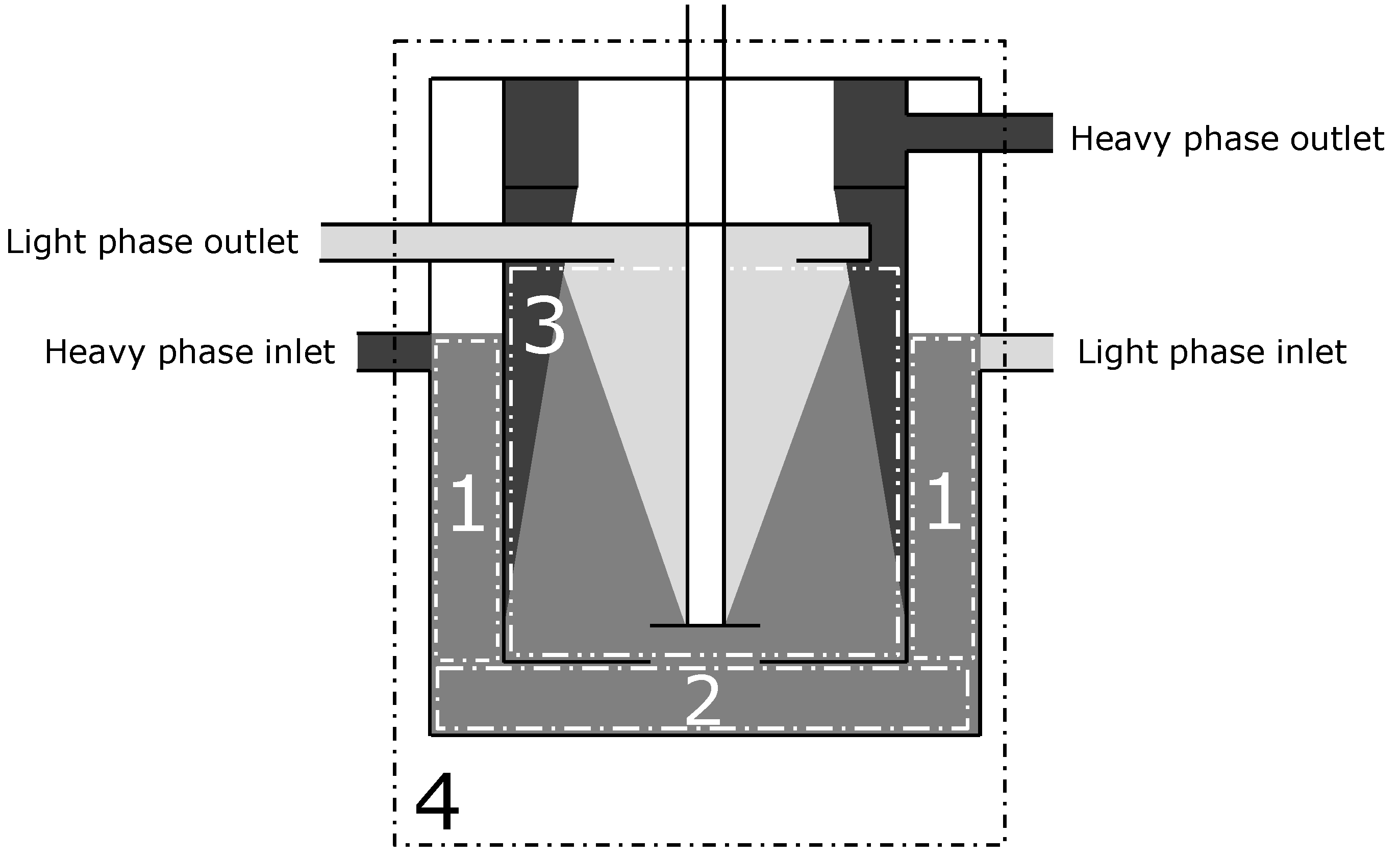
3.1. Definition of the Boundaries of the Balance Sheets

As mentioned above, the ACC was divided in four balance volume compartments for modelling. First, their boundaries were defined (see Figure 1). The first compartment included the annular region of the ACC (Figure 1, compartment 1). The bottom section of the ACC between the outer, static cylinder and the inner, rotating cylinder was defined as the second area (Figure 1, compartment 2). The third balance area consisted of the inner area of the inner, rotating cylinder (Figure 1, compartment 3). The fourth balance sheet was set to include the whole ACC (Figure 1, compartment 4).

3.2. Creation of the Model Equations

For modeling, the following assumptions were made. For the annular region it was assumed that dispersion occurs instantaneously, and a constant average drop diameter is present in the whole annular region. Furthermore, backmixing effects in the axial direction were excluded here. With these assumptions, the first balance sheet compartment (Figure 1, compartment 1) could be modelled like a plug flow reactor according to Equation (2), with c as concentration of the transferred component in one phase, t as time, v as mean velocity and z as the axial coordinate.
c t = c · v z + c ˙ s o u r c e s c ˙ s i n k s
The second balance sheet area (Figure 1, compartment 2) was seen as a perfectly mixed region without concentration gradients or variations in mean drop diameter. Due to the assumed, ideal mixing and the continuous inlet and outlet flows in this balance sheet area, it was modelled as a continuous stirred tank reactor. Equation (3) shows the underlying model equation with n as the amount of substance.
d n d t = n ˙ i n n ˙ o u t + n ˙ s o u r c e s n ˙ s i n k s
Like the assumed, instantaneous dispersion in balance sheet area 1, coalescence in balance sheet 3 is also assumed as instantaneous and complete. The resulting interface area is small compared to the interface area in balance sheet compartments 1 and 2. Therefore, the mass transfer in here is negligible. Balance sheet area 4 as the whole ACC was used for plausibility checks using the mass balance of all input and output streams of the ACC.
The assumptions of the absent backmixing in area 1 and the ideal mixing in area 2 are only fulfilled to a certain degree. As errors resulting from both assumptions have contrary effects, the cumulated error is expected to be low. The same applies for the instantaneous dispersion in balance sheet area 1 and the instantaneous coalescence in balance sheet area 3.
For the model, the distribution coefficient K is defined as the ratio of the concentration of the organic phase divided by the concentration of the aqueous phase. Positive values for mass transfer correspond to a mass transfer from the aqueous phase into the organic phase. With these definitions and the limitation to the steady state, mass transfer in the boundaries for the balance sheet area 1 is described by Equation (4). It should be noted that in this equation and the following equations, the time t is the control variable. It is equivalent to the position of a volume element in the ACC. A volume element enters the ACC at t = 0 and leaves at t = τ ¯ with τ ¯ representing the average residence time. Time stamp t must not be mistaken as time for dynamic modeling of unsteady states or processes.
n ˙ t = A · β t o t · K · c a q t c o r g t
Extending mass balance equations by the equation for mass transfer, the concentration of the transferred component in the aqueous phase, dependent on the position in the ACC, can be expressed mathematically. With the molar concentration and the specific interface area a as the ratio of interface area divided by volume, Equation (5) results for balance sheet 1.
c a q t = c a q , i n a · β t o t · K · c a q t c o r g t   d t
Moreover, c o r g t is eliminated in Equation (5) by extension of Equation (5) by the conservation of mass (Equation (6)). The resulting Equation (7) was implemented in python code and solved with different methods of the solve_IVP function from the library SciPy. With the hereby obtained results for c a q t , Equation (6) was also used to calculate c o r g t .
c o r g t = c o r g , i n + c a q , i n c a q t · V a q V o r g
c a q t = c a q , i n a · β t o t · K · c a q t c o r g , i n c a q , i n c a q t · V a q V o r g   d t
The dependence of the solving method, the resolution, and the error for the numerical solution of the ODE was tested and the resulting error was found to be reasonably low for 10,000 arithmetic operations. The different solutions obtained from different solver methods are displayed in Figure 2 for an exemplary simulation of balance sheet area 1. The concentration profiles of both phases are plotted over time. Here, time represents a spatial coordinate along a hypothetical streamline through the ACC.
It is obvious from the first column of Figure 2 that the methods RK23, RK45 and DOP853 do not converge. In contrast, the methods Radau, BDF and LSODA result in converging solutions (Figure 2, second column). RK23, RK45 and DOP853 have in common that they are explicit Runge–Kutta methods. The converging methods Radau, BDF and LSODA are working with implicit Runge–Kutta methods or implicit multi-step methods. For further simulations, the method BDF was used.
For determination of the mean residence time, the knowledge of the liquid hold-ups within the boundaries of the balance sheet areas is essential. Considering previous work on the topic (e.g., [12,13]), the annular region is expected to be mainly filled with liquid, only containing a small amount of gaseous phase. When the gaseous phase is neglected, the liquid volume equals the entire volume within the boundaries of balance sheet area 1 V 1 . Therefore, the mean residence time is τ ¯ 1 = V 1 / V ˙ and the output concentration of balance sheet area 1 is c a q τ ¯ 1 , resp. c o r g τ ¯ 1 . These concentrations are the input concentrations for balance sheet area 2.
Since here the model of a CSTR is used, the concentration in the output streams equals the concentration in the bulk. Therefore, mass transfer can be expressed as Equation (8).
n ˙ = A · β t o t · K · c a q , o u t c o r g , o u t
Additionally, the expression for transferred mass as the product of flow rate of one phase multiplied by the concentration difference between output and input of this phase is applicable. Extending Equation (8) by this connection gives Equation (9).
c o r g , o u t = β t o t · A · K · c a q , o u t + V ˙ o r g · c o r g , i n V ˙ o r g + β t o t · A
Since the conservation of mass applies, the sum of the products of concentration multiplied with the flow rate must be equal for input and output streams. By rearranging this connection, c o r g , o u t can be eliminated from Equation (9). Equation (10) is obtained, where ϕ is the volume ratio of organic phase to aqueous phase. Since the estimation of liquid hold-ups in ACCs is complex [12,14], the volume ratio of organic phase to aqueous phase is equated with the flow rate ratio of organic phase to aqueous phase. Rearranging Equation (10) to isolate c a q , o u t gives the model equation for the output concentration of the aqueous phase, which was implemented in python code. For calculation of the output concentration of the organic phase with python, Equation (11) was used.
c a q , o u t = c a q , i n + ϕ · c o r g , i n ϕ · β t o t · A · K · c a q , o u t + V ˙ o r g · c o r g , i n V ˙ o r g + β t o t · A
c o r g , o u t = c o r g , i n + 1 ϕ · c a q , i n 1 ϕ · c a q , o u t
As mentioned above, mass transfer is neglected in balance sheet area 3, so the output concentration and therefore the whole ACC are the same as the ones of balance sheet area 2. For balance sheet area 4, input and output streams of the ACC have to comply with the law of conservation of mass.

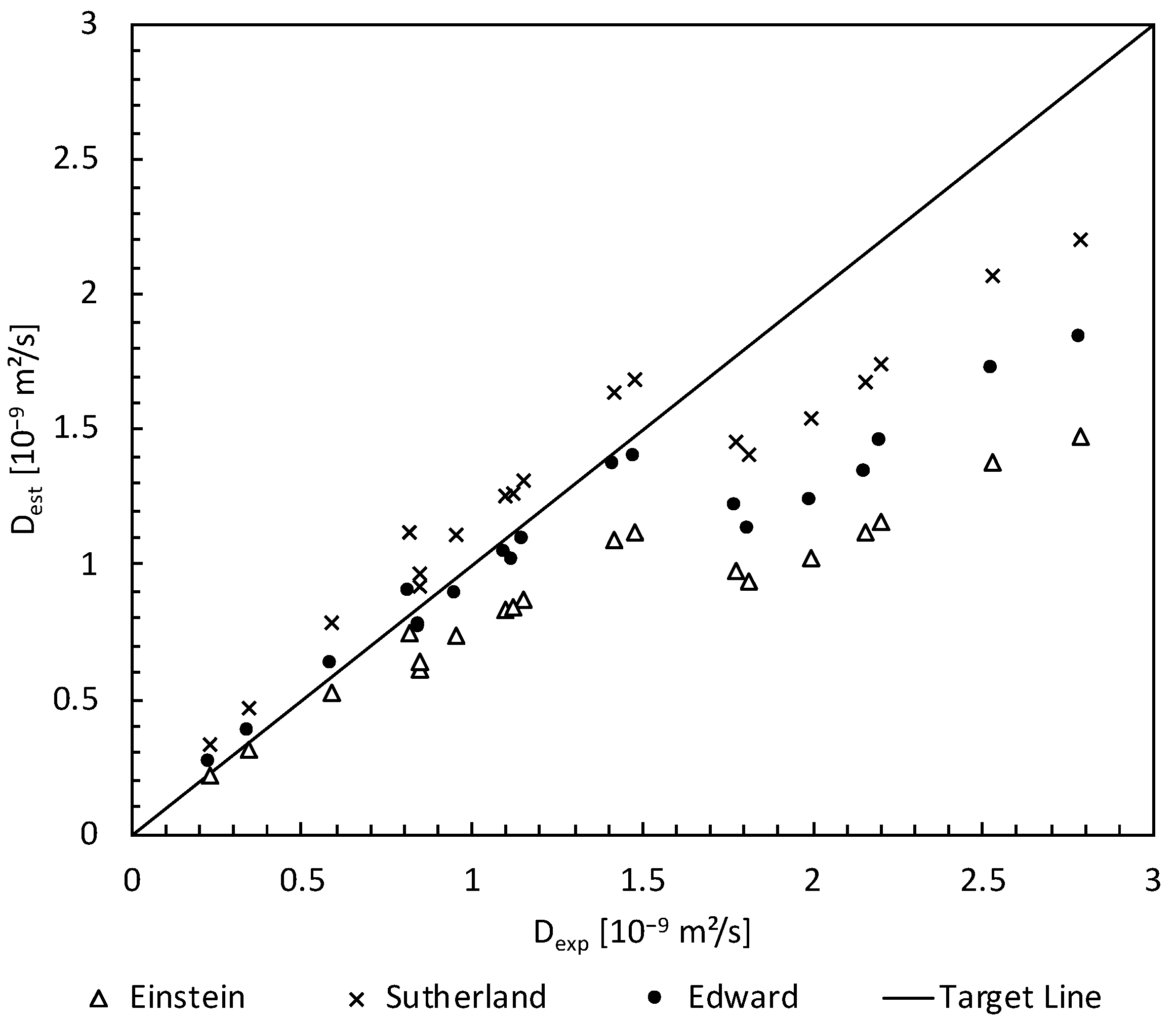
3.3. Estimation of Parameters Contributing to Mass Transfer

In order to obtain results from the model, mass transfer coefficients and (specific) interface area have to be estimated. First, the total mass transfer coefficient β t o t can be expressed through the mass transfer coefficients in the organic phase β o r g and the aqueous phase β a q according to Equation (12).
β t o t = 1 1 β o r g + K β a q
To obtain the phase-specific mass transfer coefficients, Sherwood number (Sh) correlations were used. The limited ranges of validity of these correlations have to be considered. The basis for this approach is the definition of the Sherwood number in Equation (13). For the continuous phase, the correlation of the Sherwood number with the Reynolds (Re) and Schmidt (Sc) number is shown in Equation (14) [15]. In this equation, D is the diffusion coefficient and l the characteristic length. The Reynolds and Schmidt number can be obtained from operating conditions, geometrical data of the ACC and physical properties of the components.
β = S h · D l
S h = 2 π · R e · S c
For the disperse phase, the corresponding correlation is shown in Equation (15) [16]. During mass transfer, a single drop of the disperse phase travels through the ACC and changes its concentration continuously due to mass transfer with the continuous phase. Hence, this drop is in an unsteady state. Therefore, the Fourier number (Fo), a non-dimensional number for unsteady heat and mass transfer processes, is required, even if the model is limited to the steady state. The Fourier number can be calculated with operating conditions, physical properties of the components and the mean drop diameter.
S h = 2 3   F o
Because these correlations are based on investigations on bulk concentrations, it is valid to use bulk concentrations in the model equations above. Additionally, it is assumed that the continuous phase is always the aqueous phase, while the organic phase is the dispersed one. This is the case for most operating conditions and systems of components [17].
Calculation of the Schmidt and Fourier number requires knowledge of the diffusion coefficient. Since the diffusion coefficient is not as widely accessible for many compounds as other physical properties, methods from Einstein, Sutherland and Edwards for prediction of diffusion coefficients are used and compared with experimental data.
Einstein [18] proposed to calculate diffusion coefficients in analogy to the frictional force in Stokes’ law [19] according to Equation (16). Sutherland [20] published the same equation as Einstein but limited it to the borderline case of zero friction. He described the other borderline case of dominating friction with Equation (17). In these equations, r is the radius of the diffusing component, k B the Boltzmann constant, T the temperature and η the dynamic viscosity. The difference between these two equations lies in the numerical value in the denominator. Edward [21] tried to cover the range between the two limiting cases and proposed a range of 2.2–6.0 for numerical values in the denominator, depending on the radius of the diffusing component.
D = k B · T 6   π · η · r
D = k B · T 4   π · η · r
The determination of the size of the diffusing component is challenging because the diffusing component is perfectly spherical only in exceptional cases. Additionally, hydrate shells or similar phenomena further complicate the determination of the radius. For this reason, the use of an equivalent radius is necessary. A suitable equivalent radius is the van der Waals radius, which can be determined using group contribution method by Edward [21] and Bondi [22] for the van der Waals volume and the assumption of a spherical shape of the volume.
Misek [10] and Berger [11] published experimental datasets for diffusion coefficients, which are limited to specific systems of components, limited concentration ranges and three temperatures. These data sets were measured in a diffusion cell using the diaphragm method after Stokes. For estimation of diffusion coefficients, the described methods of Einstein, Sutherland and Edward were used. To have comparable experimental and estimated datasets, the values were estimated using the same temperatures and systems of components used by Misek and Berger for comparison (Figure 3).
All utilized methods show good agreement with the experimental data. Judged by mean square errors, the method of Sutherland (Equation (17)) shows best agreement with experimental data. For this reason, the method of Sutherland is used for estimating diffusion coefficients in the model. Furthermore, it is noticeable that diffusion coefficients above 1.7 × 10⁻⁹ m2/s are consistently underestimated. The underestimated diffusion coefficients have in common that they are for diffusion in a solvent with low polarity.
The interfacial area, identified as the second crucial parameter for simulation, can be calculated from the Sauter mean diameter d P , 32 and the volume fraction of the dispersed phase ϕ d i s p according to Equation (18) [23].
a = 6   ϕ d i s p d P , 32
The simplification mentioned above, that the volume fraction of the dispersed phase equals the flow rate fraction of the dispersed phase, is applied. Thus, ϕ d i s p can be obtained from operating parameters. A more challenging task is the estimation of the Sauter mean diameter. In Taylor–Couette reactors, very similar, although not identical, flow patterns as in ACCs can be found. Thus, more information on these systems is available and considered for the situation in ACCs. Haas [24] investigated the drop size distributions in Taylor–Couette reactors and found that the mean drop diameter d ¯ P can be described as follows:
d ¯ P d R , O D = 150 · W e 0.65 · R e 0.2 · d R , O D d R , I D 0.5
The Weber (We) and Reynolds number can be obtained from operating conditions and physical properties. The diameter of the inner rotor of the ACC d R , I D and of the outer rotor d R , O D can be measured after disassembly of the machine. Haas also found a correlation between the mean drop diameter and the maximum drop diameter. Clay [25] found regularities in ratios of different percentiles of the drop size distributions in Taylor–Couette reactors. Calabrese [26] and Hesketh [27] confirmed these regularities and added the Sauter mean diameter as an aim of their investigations. By combining these findings, an average ratio of the Sauter mean diameter and the mean drop diameter can be approximated as 1.

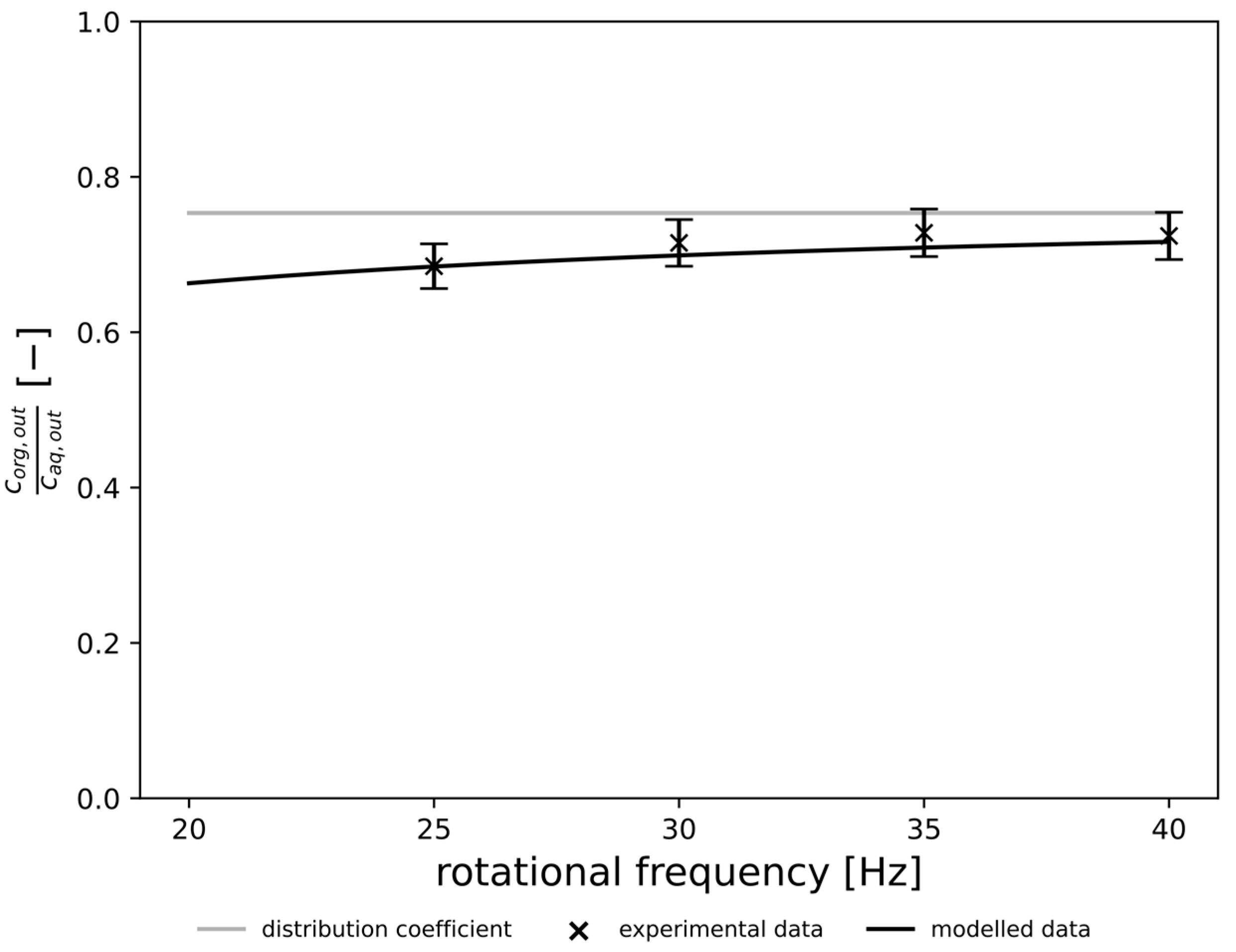
3.4. Validation of Simulated Results with Experimental Data

The steady state of the ACC was reached after 5 min. Thus, sampling was done 5 min after start-up of the ACC for all experiments. For validation purposes experimental data were collected and compared to simulated data. Geometrical parameters were predefined by the type of ACC used in the experiments and obtained directly by measuring the dimensions of the components. A range of rotational frequencies, temperatures, flow rates, flow rate ratios and different systems of components were tested and simulated. Experimental and simulated data of the output concentration ratio for rotational frequencies of 20–40 Hz are shown in Figure 4. Additionally, the distribution coefficient is shown as a grey line. The remaining operating conditions were kept constant at a temperature of 20 °C, a flow rate of 150 mL/min and a flow rate ratio of 1. The used system of components was water–acetone–toluene. Experimental data show very good agreement with simulated data over the whole range of rotational frequencies.
Temperature was varied in the range of 10–30 °C. The experimental and simulated data of the output concentration ratio are shown in Figure 5. The remaining parameters were kept constant at a rotational frequency of 30 Hz, a flow rate of 150 mL/min and a flow rate ratio of 1. Good agreement of experimental and simulated data can be seen for the variation of temperature as well. A slight underestimation of the influence of the temperature is visible in the simulated data.
As the outlet temperature was influenced by the flow rate, the flow rate ratio and the set of components, the comparison between experimental and simulated data is not meaningful. Variation in temperature strongly affects the distribution coefficient (as can be seen in the published physical properties [10,11]). Since the distribution coefficient is a major parameter for mass transfer, mass transfer is also strongly affected by varying temperatures.

4. Model Validation and Discussion

The non-converging behavior of the explicit Runge–Kutta methods is a strong indicator that the present ODE is of a stiff kind. Stiff ODEs are best solved with implicit methods as BDF, which show converging behavior in these cases [28,29].
The comparison of the estimated diffusion coefficients showed good agreement regarding all methods with a slightly better agreement for the method of Sutherland. All approaches have in common that they underestimate diffusion coefficients in solvents with low polarity. It can be presumed that the applied methods offer more precise estimations for polar solvents than for less polar solvents. Furthermore, comparison of mass transfer coefficients of organic phases and aqueous phases calculated during the simulations shows that the mass transfer coefficient for the organic phase is lower than the mass transfer coefficient for the aqueous phase. The difference between the two mass transfer coefficients is about four orders of magnitude. This is in accordance with the usual observations, locating the mass transfer limitation on the side of the disperse phase, which is in this case expected to be the organic phase.
Investigation of the equilibration time of the ACC prior to the experimental model validation showed a steady state after 5 min, which is in accordance with the observations of Schuur [14]. Standard deviation of the output concentration determined within three repeated experiments with identical parameters was 4.2% and therefore, moderate. Improved accuracy could be achieved with a more precise analytical method as could be seen in missing amounts of mass in the mass balances during a plausibility check and a more precise temperature management.
Model validation for a range of rotational frequencies and temperatures was successful. Both experimental and simulated data showed an enhanced mass transfer for increased rotational frequency. This is the expected behavior, since a higher rotational frequency leads to a higher shear force in the annular gap, which results in smaller drop sizes and therefore, a larger interfacial area. This is in accordance with Schuur [14] and Kraai [30] for the investigated range of rotational frequencies. The comparison of experimental and simulated data for different temperatures showed good agreement with a slight underestimation of the influence of temperature in our simulations. Temperature is indirectly affecting mass transfer by its influence on various parameters relevant for mass transfer during extraction (e.g., diffusion coefficients, viscosities, interfacial tensions). The effect of an increasing temperature on these parameters is throughout enhancing mass transfer, which is in accordance with the experimental results. The slight underestimation of the influence of the temperature is assumed to be caused by the differences in temperatures in the outlet flows and the temperatures for the published physical properties. Even if distribution coefficients were adapted to the actual temperatures, all remaining physical properties were not adjusted. Therefore, it could be shown that the model delivers results in accordance with experimental results with the presented accuracy.
Comparison of experimental and simulated data for flow rate and flow rate ratio variation did not result in conclusive correlations. The most plausible reason is that mass transfer limitation effects cannot be observed because of dominant effects of heat transfer limitation. The observations of the influence of flow rate and flow rate ratio indicate a limitation in heat transfer from the tempering jacket. The effects of a limitation in mass transfer are over-compensated by the effects of the limitation in heat transfer. For upcoming investigations using this model, it can be recommended to repeat the validation of the remaining parameters with improved temperature management and a more accurate analytical method. The attempted validation for different systems of components could not be finalized due to limitations in the analytical method. Lastly, it should be mentioned that the intrinsic constraints should be kept in mind while using the model. Due to the chosen approach for modelling, the applicability does not include dynamic processes, non-isothermal processes or reactive extraction processes.

5. Conclusions

In this article, a model for mass transfer in ACCs was established. One-dimensional modeling of mass transfer processes during physical extractions in ACCs was done successfully based on geometrical data of the ACC, operating conditions of the ACC and physical properties of the components. Behavior of the model was investigated by running python-based simulations. Experiments were conducted and compared to the results of the simulations for validation purposes. It could be shown that over the tested range of rotational frequencies and temperatures, the simulated results matched the experimental results. During validation of flow rates and flow rate ratios, phenomena could be observed that indicate a limitation in heat transfer. Therefore, not only is mass transfer a limiting process but also heat transfer. Interferences of the effects caused by mass and heat transfer limitations prevented a reliable validation of the parameters flow rate and flow rate ratio.

Author Contributions

Conceptualization, P.M.R. and B.C.S.; methodology, P.M.R. and B.C.S.; software, P.M.R.; validation, P.M.R.; chemical analysis, P.M.R. and C.K.W.; formal analysis, P.M.R. and B.C.S.; writing—original draft preparation, P.M.R.; writing—review and editing, C.K.W. and B.C.S.; visualization, P.M.R. and B.C.S.; supervision, C.K.W. and B.C.S.; project administration, B.C.S.; funding acquisition, B.C.S. All authors have read and agreed to the published version of the manuscript.

Funding

This research received no external funding.

Data Availability Statement

Not applicable.

Conflicts of Interest

The authors declare no conflict of interest.

References

  1. Hamamah, Z.A.; Grützner, T. Liquid-Liquid Centrifugal Contactors: Types and Recent Applications—A Review. ChemBioEng Rev. 2022, 9, 286–318. [Google Scholar] [CrossRef]
  2. Seyfang, B.C.; Klein, A.; Grützner, T. Extraction Centrifuges—Intensified Equipment Facilitating Modular and Flexible Plant Concepts. ChemEngineering 2019, 3, 17. [Google Scholar] [CrossRef] [Green Version]
  3. Wang, Y.; Du, C.; Yan, Z.; Duan, W.; Deng, J.; Luo, G. Liquid-liquid flow and mass transfer characteristics in a miniaturized annular centrifugal device. Chem. Eng. J. 2022, 431, 3. [Google Scholar] [CrossRef]
  4. Schuur, B.; Jansma, W.J.; Winkelman, J.G.M.; Heeres, H.J. Determination of the interfacial area of a continuous integrated mixer/separator (CINC) using a chemical reaction method. Chem. Eng. Process. 2008, 47, 1484–1491. [Google Scholar] [CrossRef] [Green Version]
  5. Kadam, B.D.; Joshi, J.B.; Koganti, S.B.; Patil, R.N. Dispersed phase hold-up, effective interfacial area and Sauter mean drop diameter in annular centrifugal extractors. Chem. Eng. Res. Des. 2009, 87, 1379–1389. [Google Scholar] [CrossRef]
  6. Nilsson, M. Combining Experiments and Simulations of Extraction Kinetics and Thermodynamics in Advanced Separation Processes for Used Nuclear Fuel; Technical Report; University of California: Irvine, CA, USA, 2018. [Google Scholar] [CrossRef] [Green Version]
  7. Patra, J.; Pandey, N.K.; Kamachi Muduli, U.; Natarajan, R.; Joshi, J.B. Hydrodynamic Study of Flow in the Rotor Region of Annular Centrifugal Contactors Using CFD Simulation. Chem. Eng. Commun. 2012, 200, 471–493. [Google Scholar] [CrossRef]
  8. Wardle, K.E. Hybrid Multiphase CFD Simulation for Liquid-Liquid Interfacial Area Prediction in Annular Centrifugal Contactors. Proc. Glob. 2013, 2013, 7650. [Google Scholar]
  9. Wardle, K.E.; Weller, H.G. Hybrid Multiphase CFD Solver for Coupled Dispersed/Segregated Flows in Liquid-Liquid Extraction. Int. J. Chem. Eng. 2013, 2013, 128936. [Google Scholar] [CrossRef]
  10. Misek, T.; Berger, R.; Schörter, J. Standard Test Systems for Liquid Extraction, 2nd ed.; European Federation of Chemical Engineering by Institution of Chemical Engineers: Rugby, UK, 1985. [Google Scholar]
  11. Berger, R.; Hampe, M.J.; Schröter, J. Neue Testsysteme für die Flüssig/Flüssig-Extraktion. Chem. Ing. Tech. 1992, 64, 1044–1046. [Google Scholar] [CrossRef]
  12. Duan, W.; Cao, S. Determination of the Liquid Hold-up Volume and the Interface Radius of an Annular Centrifugal Contactor using the Liquid-Fast-Separation Method. Chem. Eng. Commun. 2016, 203, 548–556. [Google Scholar] [CrossRef]
  13. Li, S.; Duan, W.; Chen, J.; Wang, J. CFD Simulation of Gas-Liquid-Liquid Three-Phase Flow in an Annular Centrifugal Contactor. Ind. Eng. Chem. Res. 2012, 51, 11245–11253. [Google Scholar] [CrossRef]
  14. Schuur, B.; Kraai, G.N.; Winkelman, J.G.M.; Heeres, H.J. Hydrodynamic features of centrifugal contactor separators: Experimental studies on liquid hold-up, residence time distribution, phase behavior and drop size distributions. Chem. Eng. Process. 2012, 55, 8–19. [Google Scholar] [CrossRef]
  15. Clift, R.; Grace, J.R.; Weber, M.E. Bubbles, Drops, and Particles; Academic Press: New York, NY, USA, 1978. [Google Scholar]
  16. Brauer, H. Unsteady State Mass Transfer trough the Interface of Spherical Particles—II: Discussion of results obtained by theoretical methods. Int. J. Heat Mass Transf. 1978, 21, 455–465. [Google Scholar] [CrossRef]
  17. Mersmann, A.; Kind, M.; Stichlmair, J. Thermische Verfahrenstechnik. Grundlagen und Methoden, 2nd ed.; Springer: Berlin/Heidelberg, Germany, 2005. [Google Scholar] [CrossRef]
  18. Einstein, A. Über die von der molekularkinetischen Theorie der Wärme geforderte Bewegung von in ruhenden Flüssigkeiten suspendierten Teilchen. Ann. Phys. 1905, 322, 549–560. [Google Scholar] [CrossRef] [Green Version]
  19. Stokes, G.G. On the Effect of the Internal Friction of Fluids on the Motion of Pendulums. Trans. Camb. Philos. Soc. 1851, 9, 8–106. [Google Scholar]
  20. Sutherland, W. A dynamical theory of diffusion for non-electrolytes and the molecular mass of albumin. Lond. Edinb. Dublin Philos. Mag. 1905, 9, 781–785. [Google Scholar] [CrossRef] [Green Version]
  21. Edward, J.T. Molecular volumes and the Stokes-Einstein equation. J. Chem. Educ. 1970, 47, 261–270. [Google Scholar] [CrossRef]
  22. Bondi, A. van der Waals Volumes and Radii. J. Phys. Chem. 1964, 68, 441–451. [Google Scholar] [CrossRef]
  23. Westerterp, K.R.; Van Swaaij, W.P.M.; Beenackers, A.A.C.M. Chemical Reactor Design and Operation, 2nd ed.; Wiley: Chichester, UK, 1987. [Google Scholar]
  24. Haas, P.A. Turbulent dispersion of aqueous drops in organic liquids. AIChE J. 1987, 33, 987–995. [Google Scholar] [CrossRef]
  25. Clay, P.H. The mechanism of emulsion formation in turbulent flow. Proc. Ned. Akad. Wet. 1940, 43, 852–865. [Google Scholar]
  26. Calabrese, R.V.; Chang, T.P.K.; Dang, P.T. Drop breakup in turbulent stirred-tank contactors. Part I: Effect of dispersed-phase viscosity. AIChE J. 1986, 32, 657–666. [Google Scholar] [CrossRef] [Green Version]
  27. Hesketh, R.P.; Fraser Russell, T.W.; Etchells, A.W. Bubble size in horizontal pipelines. AIChE J. 1987, 33, 663–667. [Google Scholar] [CrossRef]
  28. Strehmel, K.; Weiner, R.; Podhaisky, H. Numerik Gewöhnlicher Differentialgleichungen. Nichtsteife, Steife und Differential-Algebraische Gleichungen, 2nd ed.; Vieweg+Teubner: Wiesbaden, Germany, 2012. [Google Scholar] [CrossRef]
  29. The SciPy Community. Scipy.Integrate.Solve_Ivp—SciPy v1.10.1 Manual. Available online: https://docs.scipy.org/doc/scipy/reference/generated/scipy.integrate.solve_ivp.html#scipy.integrate.solve_ivp (accessed on 20 March 2023).
  30. Kraai, G.N.; Schuur, B.; van Zwol, F.; van de Bovenkamp, H.H.; Heeres, H.J. Novel highly integrated biodiesel production technology in a centrifugal contactor separator device. Chem. Eng. J. 2009, 154, 384–389. [Google Scholar] [CrossRef] [Green Version]
Figure 1. Section view of a schematic ACC with the four balance sheet compartments marked as dash-dotted rectangles.
Chemengineering 07 00059 g001
Figure 2. Comparison of the concentration profiles for an exemplary ACC simulation resulting for different ODE solver methods.
Chemengineering 07 00059 g002
Figure 3. Comparison of published datasets for experimental diffusion coefficients Dexp (taken from Misek [10] and Berger [11]) with their corresponding estimated diffusion coefficients Dest using the methods of Einstein, Sutherland and Edward (the target line corresponds to a deviation between experimental and estimated diffusion coefficients of zero).
Chemengineering 07 00059 g003
Figure 4. Output concentration ratio in dependence of rotational frequency.
Chemengineering 07 00059 g004
Figure 5. Output concentration ratio in dependence of temperature.
Chemengineering 07 00059 g005
Disclaimer/Publisher’s Note: The statements, opinions and data contained in all publications are solely those of the individual author(s) and contributor(s) and not of MDPI and/or the editor(s). MDPI and/or the editor(s) disclaim responsibility for any injury to people or property resulting from any ideas, methods, instructions or products referred to in the content.

