Comparison of the Dynamic and Thermal Behavior of Different Ideal Flow Crystallizers

Abstract

In this simulation study, we compare the dynamics and thermal behavior of different ideal flow crystallizers. The first step in creating mathematical models for the crystallizers was the implementation of the population balance equation. The population balance equation was completed with mass balance equations for the solute and the solvent as well as in the case of non-isothermal crystallizers with an energy balance equation. The solution to the population balance equation, which is a partial differential equation, can only be performed numerically. Using the method of moments, which calculates the moments of the population density function, gives a mathematically simpler model for simulating and analyzing the crystallizers. All crystallizers studied are considered mixed suspension and mixed product crystallizers. In this simulation study, the investigated crystallizers are the batch mixed suspension and mixed product isothermal crystallizer, the batch mixed suspension and mixed product non-isothermal crystallizer, and the continuous mixed suspension and mixed product removal (CMSMPR) non-isothermal crystallizer equipped with a cooling jacket. We consider citric acid as the solid material to be crystallized, and a water–glycol system is used as a cooling medium. Considering the nucleation kinetics, we applied both primary and secondary nucleation. In the case of a crystal growth kinetic, we assumed a size-independent growth rate. The highest expected value and the variance of the crystal product occur in the isotherm batch case, which can be explained by the high crystallization rate caused by the high supersaturation. Contrary to this, in the non-isothermal batch case, the final mean particle size and variance are the lowest. In continuous mode, the variance and mean values are between the values obtained in the two other cases. In this case, the supersaturation is maintained at a constant level in the steady state, and the average residence time of the crystal particles also has an important influence on the crystal size distribution. In the case of non-isothermal crystallization, the simulation studies show that the application of the energy balance provides different dynamics for the crystallizers. The implementation of an energy balances into the mathematical model enables the calculation of the thermal behavior of the crystallizers, enabling the model to be used more widely.

1. Introduction

The modeling of particulate systems is often challenging due to many model parameters. This is especially true in the case of crystallization processes, where large numbers of particles are present, and their size distribution changes over time and the three spatial dimensions. A large number of particles are often handled as a population and modeled by the population balance method. In practice, the temperature of crystallizers may be the critical parameter for obtaining adequate products; the mathematical models should be completed with an energy balance accounting for the non-isothermal behavior of the system. Many applications of the population balance model developed for modeling crystallizers can be found in the literature. In general, the authors investigate unique crystallizers with given flow and thermodynamic characteristics, and there are only a few studies that compare the behavior of different crystallizers. Ma et al. examined the effect of the different operational parameters (cooling rate, seeding temperatures, seeding load and shape) on the crystal size distribution. They also emphasize the need to apply simulation-based tools to develop new technologies. The applied model is called a morphological population balance, containing multi-spatial crystal development. Nucleation, agglomeration and breakage are also included [1]. Yang et al. investigated the crystallization of indomethacin. The equation of population balance contains the terms of nucleation, growth and aggregation but no breakage. The model parameters were identified by comparing the simulation to experimental results. Additionally, the effect of the operation parameters (stirring rate and temperature) was examined [2]. The chocolate roller size distribution calculated by Khajehesamedini et al. mainly depends on the velocities and grinding parameters. The model, including a breakage term, was validated against industrial data [3]. The high-shear granulation was modeled by Muthancheri et al., where the crystal growth can be divided into different groups according to the temporal behavior of the granulates. The authors used a reduced-order population balance model with lumped liquid and gas dimensions. Aggregation and breakage were also included, and the population balance equation was solved using a two-compartment modeling scheme using impeller and circulation compartments. The first-order explicit Euler integration technique was used to solve the population balance equation [4]. Bellinghausen et al. focused on the design of a high-shear granulator. A one-dimensional population balance equation was applied, including breakage and coalescence. The validation of the model is based on four different crystallizer sizes from the lab scale to a pilot plan: from 2 to 70 L [5]. However, the most important or frequent application field of population balances is related to the pharmaceutical industry. Szilagyi et al. showed methods to ensure the quality of the crystalline product by controlled crystallization. They investigated the cooling crystallization of L-ascorbic acid. A one-dimensional population balance model was applied, and cube-sized crystals were assumed. The model was solved by the high-resolution finite volume method. The model was used to compare two methods of crystal size control (direct nucleation and non-linear model predictive control). Based on the results, the quality of the control framework was generalized. Crystal breakage occurs not only when the crystals contact each other but also when they can collide with the reactor wall or the impeller blades [6]. Szilagyi and Lakatos applied a two-dimensional population balance model to simulate an MSMPR crystallizer. The model was extended to support non-linear breakage, including the collision of the crystals with the wall, impeller and other particles. The method of moments with 2D quadrature was used for the solution to the model [7]. Szilagyi et al. simulated a cascade MSMPR crystallizer structure using the population balance model. The system contained slurry recirculation. The start-up process of the system and its robustness were also examined. The model was solved by the method of moments. One of the most important characteristics of crystalline products in the pharmaceutical industry is their purity [8]. Fysikopoulos et al. developed a multi-dimensional population balance model that accounts for the chemical components of the impurities. The main focus of this research lies in the estimability of the model parameters, which were evaluated using a unique estimability framework. The other challenge arises when modeling a fluidized bed crystallizer, due to the stochastic (chaotic) nature of fluidized bed crystallization [9]. Bartsch et al. calculated the fluid flow in the usual deterministic way, while particle movement was treated by a stochastic method. The model results were compared to experimental results, and a good qualitative agreement was found. However, the complexity of the system makes the quantitative characterization more difficult. Most mathematical models presented for continuously stirred crystallizers are concentrated parameter models assuming ideal mixing. However, some examples use detailed hydrodynamic descriptions in the model [10]. Farias et al. applied a two-phase Euler–Euler model extended with a population balance model for a continuous flow crystallizer. The models were solved within the CFD software OpenFOAM using lovastatin crystallization in a coaxial crystallizer. In this case, the lattice Boltzmann method was used to solve the population balance equations [11].

One of the most commonly used simplifications in the research discussed above is the assumption of the isothermal operation mode of crystallizers. However, to describe realistic crystallization processes, it is essential to complete the model with an energy balance. Muthancheri et al. modeled a supercritical batch crystallization using CO${}_2$ as an antisolvent. Their model can accurately predict the crystal size distribution. The two-dimensional population balance equation was completed with an energy balance. The model is also coupled with the solvent removal kinetics and a drying step. The two-dimensional population balance equation was solved using the finite difference method. The model was validated against laboratory-scale experiments [12]. Another example of the application of an energy balance is shown by Ulbert and Lakatos who modeled a CMSMPR vacuum crystallizer. In that study, an energy balance was implemented for both the vapor and liquid phases. The model was solved using the method of moments [13].

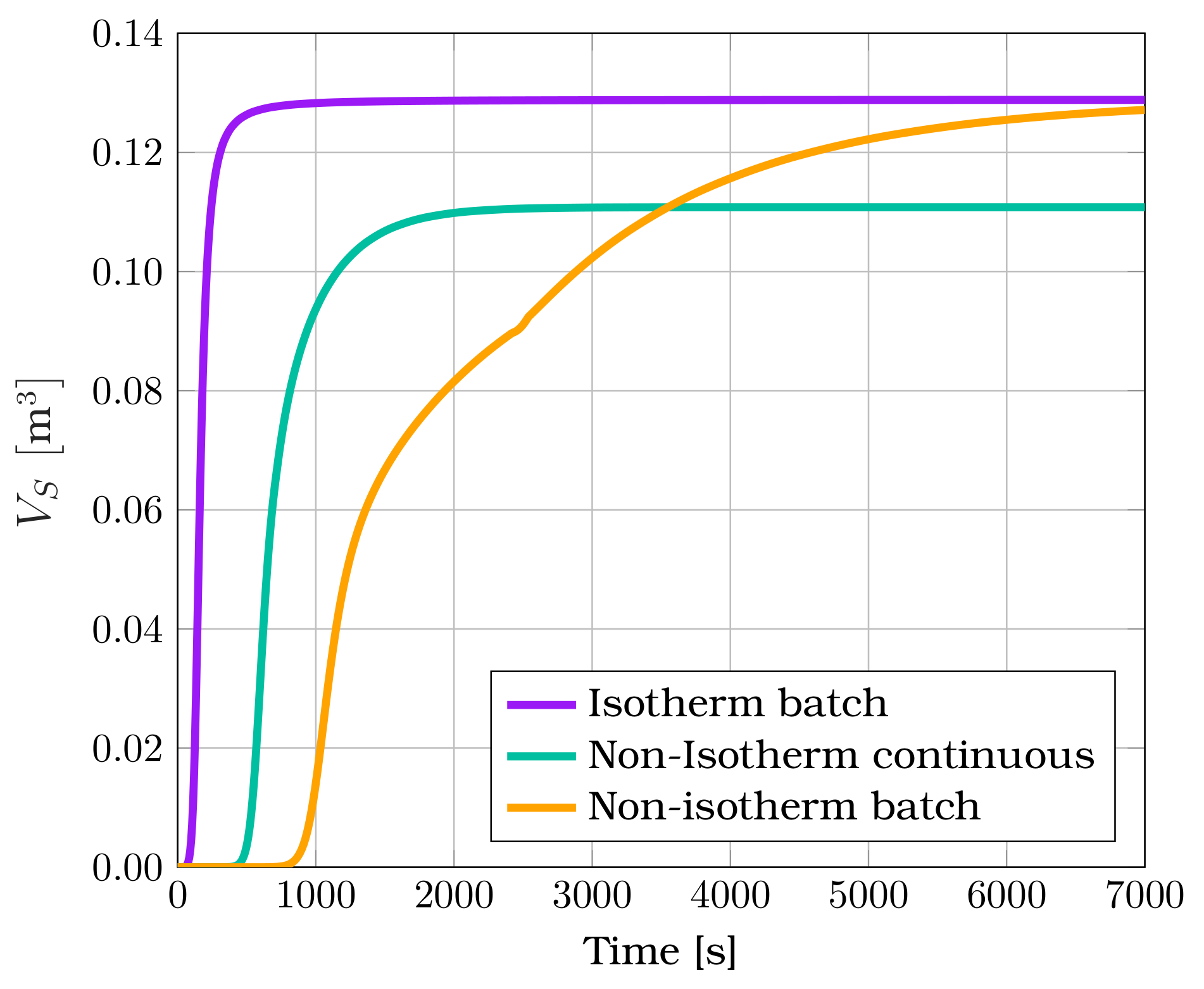
In the literature that we reviewed, we couldn’t find comparative simulation studies investigating how the product quality and dynamic behavior differ among ideal flow crystallizers with different operation modes, i.e., under batch, continuous, isothermal and non-isothermal conditions. In our research work, we carried out the following investigations. In the first case, the crystallizer works under isotherm conditions in batch operation mode. In the second case, we complete the model with an energy balance to simulate non-isothermal batch crystallization. Finally, we examined the non-isothermal continuous crystallizer. In our study, we examine the effect of the implementation of the energy balance on the crystal size distribution, crystalline product volume and solute concentration. The isothermal and non-isothermal operation modes are compared, and the advantages and disadvantages of the non-isothermal operation are highlighted.

In Section 2, the detailed model and the examined system are presented. Section 3 summarizes the model parameters and material characteristics used in the simulation studies, while, in Section 4, the results of the different operation modes are presented and investigated.

2. Mathematical Model

In the crystallizer, there is a continuous phase (solvent) and a discrete phase (crystals). The crystal particles can interact with each other and also with the continuous phase. In the population balance equation, the local change in the population density ($\mathsf{\Psi }$) is dependent on the change along coordinates (${\nabla }_r\left(\mathsf{\Psi }\dot{\mathbf{R}}\right)$) and the source terms G. The general population balance equation can be written as follows (Equation (1)) [14,15,16].

$$\frac{\partial \mathsf{\Psi }}{\partial t}+{\nabla }_r\left(\mathsf{\Psi }\dot{\mathbf{R}}\right)+G=0$$

(1)

The crystallizer is equipped with a cooling jacket. The cooling liquid is considered a water–glycol system, so a wide range of temperatures can be provided (even −50 to 190 ${}^{°}$C [17]). The crystallizer is supplied with a continuous feed, with the inlet being a hot, supersaturated citric acid solution. The outlet consists of the solution and solid crystals. During the modeling, the following assumptions were implemented:

• The suspension inside the crystallizer is perfectly mixed. The outlet stream has the same composition as the one inside the equipment.
• The working volume (V) inside the crystallizer is constant.
• Agglomeration and breakage are negligible based on [15,18].
• Bravi and Mazzarotta found that the crystal growth has a linear size dependency; however, it is not significant compared to the effect of supersaturation [19]. Therefore, we treat it as if the growth rate is independent of the size of the crystals so that we can state that every crystal grows at a similar rate.
• The volume of the crystallized solute is the same as its volume in the dissolved state; therefore, we can assume that the equation is satisfied where $V_S$ is the volume of the crystalline product, and $V_F$ is the volume of the fluid phase.
• The inlet stream does not contain any impurities or crystals.
• The heat transfer between the crystals and the solution and the crystallization heat as a heat source are negligible.
• The size distribution of the crystal particles can be described with a lognormal distribution (Equation (21)).

2.1. Population Balance Model

The crystals are treated as spherical particles; therefore, one-dimensional crystal growth was implemented. The growth rate ($v_r$) depends on the supersaturation level, which can be calculated from the mass balance of the solute. Solubility is a temperature-dependent parameter. The growth kinetics is formulated as follows (Equation (2)) [15].

$$v_r=\frac{dr}{dt}=K_G{\left[c\left(t\right)-c^{*}\left(T\left(t\right)\right)\right]}^{\omega }$$

(2)

To describe the nucleation, we should look at the solubility–supersaturation diagram of citric acid (Figure 1). Three zones can be differentiated in the diagram. In the undersaturated, or subsaturated, zone, the solvent can dissolve more solid material, while, in the unstable zone, crystals begin to form. Between the two zones, the solid concentration is higher than the solubility. This zone can be reached by creating a saturated solution at a high temperature and then cooling down to reach the metastable zone (MSZ). In addition, citric acid has two pseudo-polymorphic modifications depending on the temperature. It is in monohydrate (CAM) form under conditions below 34 ${}^{°}$C and in anhydrate (CAA) form above.

The solubility concentration is formulated as the following equation [21] (Equation (3)).

$$c_{CA}^{*}\left[\frac{kg}{kg\mathrm{water}}\right]=\left\{\begin{array}{cc}\exp \left(-120.05+\frac{3785.6}{T}+19.217\ln T\right)\hfill & \mathrm{if}T\le 34{}^{°}\mathrm{C}\hfill \\ \exp \left(-100.14+\frac{3698.7}{T}+15.794\ln T\right)\hfill & \mathrm{if}T>34{}^{°}\mathrm{C}\hfill \end{array}\right.$$

(3)

Based on this mechanism, several nucleation processes can be described. Based on the formation of the nucleus, there are homogeneous, heterogeneous, primary or secondary forms of nucleation [22]. Regardless of what causes the primary and secondary nucleation, each of them is described mathematically with one equation. The primary nucleation can be formulated by the Volmer equation (Equation (4)). In this kinetic expression, the nucleation rate is dependent on the free energy change and temperature. Moreover, it can be described with an Arrhenius type of equation [23].

$$B_{0,1}=A\exp \left(\frac{\Delta G}{RT}\right)$$

(4)

Since the free energy change in crystallization ($\Delta G$) ) is difficult to measure, instead of Equation (4), a phenomenological power law-type equation (Equation (5)) is generally used in practice [24].

$$B_{0,1}=K_{B,1}{\left[c\left(t\right)-c^{*}\left(T\left(t\right)\right)\right]}^{\vartheta }$$

(5)

The secondary nucleation includes the effect of the impeller and mainly depends on the volume of crystals formed. It can be formulated as follows (Equation (6)). Sikdar and Randolph found that the impeller speed in a citric acid crystallization has minimal effect on the secondary nucleation, or $\varsigma =0$ in our case [25].

$$B_{0,2}=K_{B,2}{V}_S^{\iota }\left(t\right)RP{M}^{\varsigma }{\left[c\left(t\right)-c^{*}\left(T\left(t\right)\right)\right]}^{\kappa }$$

(6)

The overall nucleation rate can be calculated by the sum of the rate of the primary and secondary nucleations (Equation (7)).

$$B_0=\frac{dN}{dt}=B_{0,1}+B_{0,2}$$

(7)

Table 1. Parameters of kinetic equations.

Parameters	Value	Unit	Equation
$K_{B,1}$	2.869 $·{10}^3$	$\left[\frac{\#}{{\mathrm{m}}^3\mathrm{s}}\right]$	Primary nucleation [26] (Equation (5))
$\vartheta$	1.585	$\left[-\right]$
$K_{B,2}$	1.72 $·{10}^8$	$\left[\frac{\#}{{\mathrm{m}}^3\mathrm{s}}\right]$	Secondary nucleation [27] (Equation (6))
$\iota$	0.47	$\left[-\right]$
$\varsigma$	0	$\left[-\right]$
$\kappa$	1.14	$\left[-\right]$
$K_G$	7.18 $·{10}^{-6}$	$\left[\frac{\mathrm{m}}{\mathrm{s}}\right]$	Nucleus growing velocity [27] (Equation (2))
$\omega$	1.58	$\left[-\right]$

shows the kinetic parameters of the nucleation and growth kinetic equations.

2.2. Crystallizer Model

The scheme of the cooled continuous mixed suspension mixed product removal (CMSMPR) crystallizer can be seen in Figure 2.

The crystallizer can be divided into the inner volume and the cooling jacket. There are two phases present inside the crystallizer: fluid and solid. One of the main assumptions is that the volume of the crystals formed has the same volume as the one by which the volume of the solution is decreased. $ϵ$ is defined as the ratio of the solid volume compared to the volume of the crystallizer. The symbol of $ϵ$ is formulated as follows (Equation (8)).

$$ϵ\left(t\right)=\frac{V_S\left(t\right)}{V_S\left(t\right)+V_F\left(t\right)}$$

(8)

Using this symbol, the balance equation for the solute can be written as follows (Equation (9)). The source term $R_{V_S}$ is calculated by the second moment of crystal size distribution.

$$\frac{d\left(c_F{V}_F\right)}{dt}=q{c}_0-(1-ϵ)qc-R_{V_S}{\rho }_S$$

(9)

The solvent concentration balance is as follows (Equation (10)).

$$\frac{d\left(c_W{V}_F\right)}{dt}=q{c}_{W,0}-(1-ϵ)q{c}_W$$

(10)

The calculation of the volume balance must be defined with an equation for the fluid phase volume (Equation (11)) and also for the solid phase volume (Equation (12)).

$$\frac{d{V}_F}{dt}=q-(1-ϵ)q-R_{V_S}$$

(11)

$$\frac{d{V}_s}{dt}=-ϵq+R_{V_S}$$

(12)

The source term ($R_{V_S}$) is formulated as follows (Equation (13)).

$$R_{V_S}=v_{r}3\varphi {\mu }_{2}V$$

(13)

In Equation (13), the $\varphi$ is the volumetric form factor, and the value of that in the case of the spherical particle is $\frac{\pi }{6}$ [15]. Developing the mathematical model for the crystal population is difficult because there are different sizes of crystals composing the suspension. The modeling of individual crystals by the discrete element method (DEM) is almost impossible due to their high number and different sizes. The changes in the population density function in the case of a continuous and one-dimensional system can be calculated using the following multi-variable partial differential equation by applying the assumptions in Equation (1) (Equation (14)).

$$\frac{\partial \mathsf{\Psi }\left(r,t\right)}{\partial t}+v_r\frac{\partial \chi \left(r\right)\mathsf{\Psi }\left(r,t\right)}{\partial r}=\frac{q_{in}{\mathsf{\Psi }}_{in}\left(r,t\right)}{V}-\frac{q_{out}{\mathsf{\Psi }}_{out}\left(r,t\right)}{V}+G$$

(14)

In Equation (14), the volume of the crystallizer is assumed to be constant. $\chi$ denotes the size-dependent growth rate function, and the proposed correlation was formulated by Canning and Randolph (Equation (15)) [28].

$$\chi =1+\gamma r$$

(15)

Assuming that the growth rate is size-independent, the value of $\gamma$ is 0. The inlet stream does not contain any solid phases, so ${\mathsf{\Psi }}_{in}=0$. Supposing that crystals can only enter the system by nucleation, Equation (14) can be written in the following form (Equation (16)).

$$\frac{\partial \mathsf{\Psi }\left(r,t\right)}{\partial t}+v_r\frac{\partial \mathsf{\Psi }\left(r,t\right)}{\partial r}=\frac{q\mathsf{\Psi }\left(r,t\right)}{V}+B_0\left(1-ϵ\left(t\right)\right)\delta \left(r-L_0\right)$$

(16)

There are various methods for solving partial differential equations, one of which is the method of moments. We decided to use this method because the solution to the received ordinary differential equation system is mathematically simpler. However, as with every approximate solving method, it also has a loss of information. The resulting ordinary differential equation system obtains a closed form if it includes the equations up to the third moment. The method of moments was presented first by Hulburt and Katz, and the base of this approach is that the distribution function can be transformed into an ordinary differential equation system of the different order of moments. The definition of the moments is as follows, where m denotes the order of the moments (Equation (17)) [29].

$${\mu }_m={\int }_0^{\infty }{r}^m\mathsf{\Psi }\left(r,t\right)dr\mathrm{where}m=0,1,\cdots ,k$$

(17)

By multiplying Equation (16) by the appropriate powers of the size variable and integrating it, we obtain the ordinary differential equation system of moments. The generalized equation is given in Equation (18). The $L_0$ is the size of nuclei; its powers can be considered as very small values. Thus, in the cases in which $m>0$, the last term in Equation (18) is negligible [16].

$$\frac{d{\mu }_m}{dt}=m{v}_r{\mu }_{m-1}-\frac{q}{V}{\mu }_m+B_0ϵL_0^m$$

(18)

The energy balances must be set for both the inside of the crystallizer and its jacket. In the case of the inner part, we should consider the solid and fluid volumes, the inlet and outlet streams and the heat transferred through the wall that will change the energy inside the equipment. Equations (19) and (20) describe the energy balances for the inside volume (Equation (19)) and the jacket (Equation (20)) of the crystallizer.

$$\begin{array}{c}\frac{d{T}_R\left(V_S{\rho }_S{c}_{p,CA}+V_F{c}_F{c}_{p,CA}+V_F{c}_W{c}_{p,W}\right)}{dt}=q{T}_R^{in}\left(c_W{c}_{p,W}+c_F{c}_{p,CA}\right)\\ -q(1-ϵ)T_R\left(c_W{c}_{p,W}+c_F{c}_{p,CA}\right)\\ -qϵT_R{\rho }_S{c}_{p,CA}+UF\left(T_R-T_J\right)+v_r\varphi 3{\mu }_2\Delta H_{krist}V\end{array}$$

(19)

$$\frac{d{T}_J{V}_J{\rho }_C{c}_{p,C}}{dt}=q_J{\rho }_C{c}_{p,C}{T}_J^{in}-q_J{\rho }_C{c}_{p,C}{T}_J+UF(T_R-T_J)$$

(20)

2.3. Particle Size Distribution Reconstruction

The reconstruction of the particle size distribution function is feasible by the application of various methods, such as the extended quadrature method of moments [30] or the maximum entropy method [31]. However, in this work, we used a distribution function that is often used to approximate the size distribution of crystals. The motivation behind the application of this method was its simplicity and that it can be calculated analytically from moments. The aim of the particle size distribution reconstruction is to show the differences between the different operation modes. The distribution function that was used is the lognormal distribution function given by (Equation (21)) [32].

$$\tilde{\mathsf{\Psi }}\left(r\right)=\frac{1}{r\sigma \sqrt{2\pi }}\exp \left(\frac{{\ln }^2(r-\varpi )}{2{\sigma }^2}\right)$$

(21)

The lognormal distribution was used to reconstruct the particle distribution by calculating its time-varying parameters $\varpi$ and $\sigma$ using the moments model. The moments of the population density function, obtained by solving the moments model, can be used to estimate characteristics of the population density function, such as expected value (E) and variance ($Var$). Using the values of moments, the equations for calculating the expected value and variance are given by Equations (22) and (23).

$$E=\frac{{\mu }_1}{{\mu }_0}$$

(22)

$$Var=\frac{{\mu }_2}{{\mu }_0}-E^2$$

(23)

Using the expected value and variance, the parameters of the lognormal distribution function ($\sigma ,\varpi$) can be calculated by the following equations (Equations (24) and (25)) [32].

$$\varpi =\ln \left(E\right)-\frac{1}{2}\ln \left(1+\frac{Var}{E^2}\right)$$

(24)

$${\sigma }^2=\ln \left(1+\frac{Var}{E^2}\right)$$

(25)

Together with the changing moments during the solution to the moments model, the parameters of the lognormal distribution are also determined, reconstructing the size distribution of the crystals.

3. Model Parameters and Material Characteristics

The section on the model parameters and material characteristics presents the geometric parameters of the crystallizer equipment and the determinations of the temperature and concentration-dependent material properties.

3.1. Reactor Geometry and Initial Values of the Calculation

The following table shows the geometry of the crystallizer (

Table 2. Geometry of the reactor based on [33].

Total volume (${\mathit{V}}_{\mathit{R}}$)	1.0	m${}^3$
Jacket volume ($V_J$)	0.235	m${}^3$
Heat transfer surface (F)	4.2	m${}^2$

). The equipment is a jacketed vessel with 1 m${}^3$ of nominal volume. The reactor was a standard construction, selected from a Lampart catalog, and the ID of the chosen equipment is A-2-03 [33].

The overall heat transfer coefficients (U) of the crystallizer wall were calculated based on [34], so the value of the calculated overall heat transfer coefficient was $486.5\frac{\mathrm{W}}{{\mathrm{m}}^2\mathrm{K}}$.

In the simulation study, the basic case was crystallization under isothermal conditions, where the isothermal temperature was defined as 30 ${}^{°}$C. In the case of a non-isothermal batch and continuous crystallizers, the temperature of the cooling medium entering the cooling jacket was calculated in such a way that the temperature of the crystallizer could reach the desired value. The initial concentration of the solvent and the solution was calculated with the solubility curve. In the case of non-isothermal continuous crystallizers, the inlet temperature of the cooling medium ($T_J^{in}$) is determined so that the temperature of the exit volume flow reaches 30 ${}^{°}$C.

3.2. Calculation of Temperature-Dependent Material Properties

Due to the added extension of the energy balance to the model, many more new parameters need to be given compared to in the isothermal case. The physical parameters of the solute were calculated by Aspen Plus software. The system is polaric and electrolyte in nature; therefore, the ELECNRTL property package was used to calculate density, heat capacity and solubility. This property package was chosen based on [35]. In the case of the cooling medium, only the temperature dependence is calculated ($f\left(T\right)$) because its composition remained constant. The given discrete data points are then used for fitting polynomial functions using the MATLAB curve fitting toolbox. The polynomial function has the following form (Equation (26)).

$$f\left(T\right)=a_f+b_{f}T+c_f{T}^2+d_f{T}^3+e_f{T}^4$$

(26)

Figure 3 shows the estimated and fitted data lines.

In the cases of citric acid solubility (Equation (3)), specific heat (Equation (28)), crystal density (Equation (27)) and the specific heat of water (Equation (28)), we used results [21,36] from the literature. The functions have the following form.

$${\rho }_S=\frac{1}{a+bT+c{T}^2}$$

(27)

$$c_p=a+bT+c{T}^2+d{T}^3+e{T}^4$$

(28)

4. Results and Discussion

This section summarizes the simulation results and the distribution reconstruction for the three different operation modes as well as the comparison of the results.

4.1. Simulation Results for Batch Mode and Isothermal Conditions

In this section, we show the simulation results obtained for the mixed suspension and mixed product isothermal batch crystallizer. The temperature of the crystallizer was set to 30 ${}^{°}$C, and the initial values of the state variables applied can be found in

Table 3. Initial values of the differential equation systems and operation conditions of the calculated systems.

Function	Isotherm Batch	Case Non-Isotherm Batch	Non-Isotherm Continuous	Unit
$V_F\left(0\right)$	1.0	1.0	1.0	$\left[{\mathrm{m}}^3\right]$
$V_S\left(0\right)$	0	0	0	$\left[{\mathrm{m}}^3\right]$
$c_F\left(0\right)$	774.06	774.06	774.06	$\left[\frac{\mathrm{kg}}{{\mathrm{m}}^3}\right]$
$c_W\left(0\right)$	301.53	301.53	301.53	$\left[\frac{\mathrm{kg}}{{\mathrm{m}}^3}\right]$
${\mu }_m\left(0\right)$	0	0	0	$\left[\frac{\#}{{\mathrm{m}}^{4-m-1}}\right]$
$T_J\left(0\right)$	-	50	50	$\left[{}^{°}\mathrm{C}\right]$
$T_R\left(0\right)$	-	50	50	$\left[{}^{°}\mathrm{C}\right]$
$q_j$	-	0.004	0.004	$\left[\frac{{\mathrm{m}}^3}{\mathrm{s}}\right]$
$q_r$	-	-	0.002	$\left[\frac{{\mathrm{m}}^3}{\mathrm{s}}\right]$
$T_J^{in}$	-	30	−28.28	$\left[{}^{°}\mathrm{C}\right]$
$T_R^{in}$	-	-	50	$\left[{}^{°}\mathrm{C}\right]$

. In this operation mode, the supersaturation is the largest at the start of the crystallization and can be formulated as follows (Equation (29)).

$$\Delta c=c_{CA}-c_{CA}^{*}$$

(29)

Figure 4 and Figure 5 show the simulation results.

Figure 4a shows that solute concentration ($c_F$) does not change significantly during the startup process (from 0 to ∼100 s) since nuclei are dominantly formed by the primary nucleation ($B_{0,1}$), as shown in Figure 4b. When the solid volume starts to increase significantly, the secondary nucleation ($B_{0,2}$) becomes the dominant nucleation process. Many new nuclei are formed and begin to grow ($v_r$) due to the increase in supersaturation ($\Delta c$). This will lead to a rapid decrease in the solute concentration. Finally, the rate of the crystallization process tends to decrease until the solute concentration reaches its solubility value of about ∼350 s (the solubility is 1.9017 $\frac{\mathrm{kg}}{\mathrm{kg}\mathrm{water}}$ at 30 ${}^{°}$C). The characteristic of the batch mode is that the nucleation and the growth processes stop as the actual concentration reaches solubility.

Figure 5 also shows that in the startup process; the rapid change in momentum values can only be observed after the secondary nucleation has started. As the solute concentration and supersaturation decrease, the rate of nucleation and the growth rate slow down. As a consequence, the values of the moments change only slightly.

4.2. Simulation Results for Batch Mode and Non-Isothermal Conditions

In the non-isothermal batch case, the set of governing equations was extended with the energy balances. The initial value and the operation parameters of the calculation can be seen in Table 3. Figure 6, Figure 7 and Figure 8 and show the results.

Figure 7 shows the temperature profiles over time. The cooling jacket temperature ($T_J$) decreases rapidly while the temperature of the inside volume ($T_R$) decreases gradually due to the cooling effect.

Figure 6 and Figure 8 show that the changes in concentration ($c_F$) and moments (${\mu }_i$) occur later (about 1000 s) than in the isothermal batch crystallizer since, in this case, supersaturation develops more slowly by cooling down the inside volume. The maximum supersaturation appears lower because the crystallizer temperature decreases slowly. The crystallization process stops much later (about ∼5000 s). The fracture in the curves in Figure 6 and Figure 8 are caused by the change in the solubility at 34 ${}^{°}$C.

4.3. Simulation Results for Continuous Mode and Non-Isothermal Conditions

The initial value and the operation parameters of the calculation can be seen in Table 3. Figure 9 and Figure 10 show the results.

Figure 10 shows that the crystallizer inlet stream keeps the temperature high, but the decrease in the reactor temperature is faster than in the case of the batch systems because the cooling medium’s temperature is much lower here. The nucleation and growth processes do not stop because the inlet flow maintains supersaturation. In the steady state, it is 0.1 $\frac{\mathrm{kg}}{\mathrm{kg}\mathrm{water}}$.

Figure 11 shows that during the startup process (about ∼400 s) the values of moments rapidly increase due to the initial highest value of supersaturation.

4.4. Reconstruction of Population Density Function

The reconstruction of the population density function provides an additional opportunity to compare the three operating modes. Based on the solution to the moments model, we calculated the expected value and variance of crystal size using Equations (21)–(23). Then, using Equations (24) and (25), we calculated the lognormal distribution given by Equation (21). The evolution of the size distribution of particles at different operation modes of the crystallizer can be seen in Figure 12, Figure 13 and Figure 14. The two abscissae are the time and the particle size, and the ordinate is the approximate distribution function. This figure shows the number of particles of a given size at a given moment. The expected value and variance of the distribution are shown in Figure A1, Figure A2 and Figure A3.

We can state for each case that, in the beginning, the size distribution in the small size interval increases intensively due to the primary nucleation, which produces a lot of nuclei of the size $L_0$. As time progresses, the supersaturation decreases ($\Delta c$), the formation of new crystals by primary nucleation ($B_{0,1}$) starts to slow down and the expected value (E) of the size distribution decreases rapidly. At the same time, the secondary nucleation ($B_{0,2}$) becomes significant, and the formation of new crystals (with $L_0$ size) starts to increase. As a consequence, the size distribution in the small size interval starts to increase again after reaching a minimum. Due to the secondary nucleation and formation of new crystals, the expected value of the population density function decreases after reaching a maximum.

4.5. Comparison of the Results

In the literature, many studies can be found on citric acid crystallization. Our results were compared to these, and we found that the trends in the results are consistent with the case of isotherm batch simulations [15,18,27]. Comparing the isothermal and non-isothermal operation modes, we can conclude that the differences in the evolution of the distributions are a consequence of the fact that, in the non-isothermal case, the nuclei are formed mainly by the secondary nucleation during the entire crystallization process. For this reason, we can see that the maximum of the size distribution increases continuously throughout the whole process. Since more crystals are formed, the average crystal size will be smaller than in the case of the isotherm batch crystallization.

For the comparison of the three cases in terms of crystal size distribution, the steady-state values of the expected value and the variance of the distribution were calculated (in the case of batch crystallizer, we consider the steady-state when the processes of nucleation and growth are both stopped). These values can be seen in

Table 4. The expected value and variance of the distribution in the three cases.

	Isotherm Batch	Non-Isotherm Batch	Non-Isotherm Continuous
Expected value (E)	$8.994·{10}^{-5}$	$6.772·{10}^{-5}$	$8.486·{10}^{-5}$
Variance ($Var$)	$8.047·{10}^{-9}$	$5.428·{10}^{-9}$	$7.232·{10}^{-9}$

.

The highest expected value and the variance occur in the isotherm batch case, which can be explained by the high crystallization rate caused by high supersaturation. Contrary to this, in the non-isothermal batch case, the final mean particle size and variance are the lowest. This can also be explained by the supersaturation dynamics since, in the slow-cooling crystallizer, supersaturation is present for a longer period of time but with a lower value. In continuous mode, the variance and the mean value are between the received values of the other two cases because, in this case, in addition to supersaturation, the average residence time of the crystal particles also has an important influence on the distribution.

For the comparison of the crystal volume of the operation modes, Figure 15 shows changes in the crystal volume over time in the three different cases.

Figure 15 shows that, in the isothermal and the non-isothermal batch systems, the final crystal volume is the same, which can be explained by the overall citric acid content being equal in these cases. The dynamic behavior is different because the development of supersaturation is slower due to the cooling. The value of crystal volume in continuous mode is 0.1098 m${}^3$, and, in the batch mode, the value is 0.1271 m${}^3$. On the other hand, the steady-state value is reached faster in continuous mode. This phenomenon can be explained by the fact that the temperature of the inside of the crystallizer decreases faster than in the batch system. The steady-state value of the volume fraction of the solid crystals is lower than in batch operation mode. This can be explained by the outlet stream carrying crystal seeds away. The continuous inflow of solute constantly ensures a higher value of supersaturation for nucleation and crystal growth, so these processes do not stop in the steady state, as can be seen in Figure 9b.

5. Conclusions

The aim of this study was to simulate mixed suspension and mixed product crystallizers using a population balance model completed with energy balances. Both the primary and secondary nucleation processes of crystals were considered. We examined the temporal behavior of the crystallizer and the evolution of the size distribution of the crystals over time. The crystallization process was investigated under three different operational modes. We made a comparative analysis under different operation conditions, during which the volume of the crystalline product and the particle size distribution were the examined properties. In the first case, batch operation mode under isothermal conditions was examined. In the second case, non-isothermal batch crystallization was considered by implementing energy balances for the inside volume and cooling jacket of the crystallizer. In the last case, we examined the behavior of a non-isothermal continuous crystallizer. The implementation of energy balances into the mathematical model enables the calculation of the thermal behavior of the crystallizer, permitting the model to be used more widely.

If the aim of the crystallization is to obtain a size-limited product size distribution, then batch operation mode seems to be more suitable. The continuous mode produces a wider distribution of the particle size. As a result of this study, we found that the use of an energy balance can modify the dynamic behavior of crystallizers to a great extent. This is especially important in the case of systems (industrial scale crystallizers) in which the dynamic of a temperature change determines the rate of the kinetic processes. In accordance with the previously mentioned conclusions, it can be concluded that temperature significantly affects the size distribution, so one of the possibilities for controlling the crystallizer is temperature control. The presented model and the conclusions of the examinations can be used for further studies, i.e., model predictive control of continuous cooling crystallizers or optimization of crystal size and dispersion.

References

1. Ma, C.Y.; Roberts, K.J. Morphological population balance modelling of the effect of crystallisation environment on the evolution of crystal size and shape of para-aminobenzoic acid. Comput. Chem. Eng. 2019, 126, 356–370. [Google Scholar] [CrossRef]
2. Yang, L.; Zhang, Y.; Liu, P.; Wang, C.; Qu, Y.; Cheng, J.; Yang, C. Kinetics and population balance modeling of antisolvent crystallization of polymorphic indomethacin. Chem. Eng. J. 2022, 428, 132591. [Google Scholar] [CrossRef]
3. Khajehesamedini, A.; Paggios, K.; Schmid, P.; Kindlein, M.; Briesen, H. A population balance model for the chocolate roller refining process. Adv. Powder Technol. 2021, 32, 4130–4140. [Google Scholar] [CrossRef]
4. Muthancheri, I.; Chaturbedi, A.; Bétard, A.; Ramachandran, R. A compartment based population balance model for the prediction of steady and induction granule growth behavior in high shear wet granulation. Adv. Powder Technol. 2021, 32, 2085–2096. [Google Scholar] [CrossRef]
5. Bellinghausen, S.; Gavi, E.; Jerke, L.; Barrasso, D.; Salman, A.D.; Litster, J.D. Model-driven design using population balance modelling for high-shear wet granulation. Powder Technol. 2022, 396, 578–595. [Google Scholar] [CrossRef]
6. Szilágyi, B.; Borsos, Á.; Pal, K.; Nagy, Z.K. Experimental implementation of a Quality-by-Control (QbC) framework using a mechanistic PBM-based nonlinear model predictive control involving chord length distribution measurement for the batch cooling crystallization of l-ascorbic acid. Chem. Eng. Sci. 2019, 195, 335–346. [Google Scholar] [CrossRef] [Green Version]
7. Szilágyi, B.; Lakatos, B.G. Model-based analysis of stirred cooling crystallizer of high aspect ratio crystals with linear and nonlinear breakage. Comput. Chem. Eng. 2017, 98, 180–196. [Google Scholar] [CrossRef]
8. Szilágyi, B. Modeling and analysis of MSMPR cascades involving nucleation, growth and agglomeration mechanisms with slurry recycling. Chem. Eng. Res. Des. 2021, 174, 42–56. [Google Scholar] [CrossRef]
9. Fysikopoulos, D.; Benyahia, B.; Borsos, A.; Nagy, Z.; Rielly, C. A framework for model reliability and estimability analysis of crystallization processes with multi-impurity multi-dimensional population balance models. Comput. Chem. Eng. 2019, 122, 275–292. [Google Scholar] [CrossRef]
10. Bartsch, C.; Wiedmeyer, V.; Lakdawala, Z.; Patterson, R.I.; Voigt, A.; Sundmacher, K.; John, V. Stochastic-deterministic population balance modeling and simulation of a fluidized bed crystallizer experiment. Chem. Eng. Sci. 2019, 208, 115102. [Google Scholar] [CrossRef]
11. Farias, L.F.; de Souza, J.A.; Braatz, R.D.; da Rosa, C.A. Coupling of the population balance equation into a two-phase model for the simulation of combined cooling and antisolvent crystallization using OpenFOAM. Comput. Chem. Eng. 2019, 123, 246–256. [Google Scholar] [CrossRef]
12. Muthancheri, I.; Long, B.; Ryan, K.M.; Padrela, L.; Ramachandran, R. Development and validation of a two-dimensional population balance model for a supercritical CO2 antisolvent batch crystallization process. Adv. Powder Technol. 2020, 31, 3191–3204. [Google Scholar] [CrossRef]
13. Ulbert, Z.; Lakatos, B. Simulation of CMSMPR vacuum crystallizers. Comput. Chem. Eng. 1999, 23, S435–S438. [Google Scholar] [CrossRef]
14. Ramkrishna, D. Chapter 2—The Framework of Population Balance. In Population Balances; Ramkrishna, D., Ed.; Academic Press: San Diego, CA, USA, 2000; pp. 7–45. [Google Scholar] [CrossRef]
15. Caillet, A.; Sheibat-Othman, N.; Fevotte, G. Crystallization of Monohydrate Citric Acid. 2. Modeling through Population Balance Equations. Cryst. Growth Amp; Des. 2007, 7, 2088–2095. [Google Scholar] [CrossRef]
16. Ulbert, Z. Kristályosítók Dinamikus Folyamatainak Modellezése és Szimulációja. Ph.D. Thesis, Veszprémi Egyetem Vegyészmérnöki Tudományok Doktori Iskola, Veszprém, Hungary, 2002. [Google Scholar]
17. Engineering ToolBox. Ethylene Glycol Heat-Transfer Fluid Properties. 2003. Available online: https://www.engineeringtoolbox.com/ethylene-glycol-d_146.html (accessed on 27 July 2022).
18. Févotte, G.; Alexandre and Sheibat Othman Nida, C. A population balance model of the solution-mediated phase transition of citric acid. AIChE J. 2007, 53, 2578–2589. [Google Scholar] [CrossRef]
19. Bravi, M.; Mazzarotta, B. Size dependency of citric acid monohydrate growth kinetics. Chem. Eng. J. 1998, 70, 203–207. [Google Scholar] [CrossRef]
20. Groen, H. Nucleation, Growth, and Pseudo-Polymorphic Behavior of Citric Acid As Monitored in Situ by Attenuated Total Reflection Fourier Transform Infrared Spectroscopy. J. Phys. Chem. B 2001, 105, 10723–10730. [Google Scholar] [CrossRef]
21. Apelblat, A. Citric Acid; Springer: Cham, Switzerland, 2014. [Google Scholar]
22. Ramanarayanan, K. Growth Rate Dispersion in Batch and Continuous Crystallizers. Ph.D. Thesis, Department of Chemical and Biological Engineering, Iowa State University of Science and Technology, Des Moines, IO, USA, 1982. [Google Scholar] [CrossRef]
23. Volmer, M.; Weber, A. Keimbildung in üBersättigten Gebilden. Z. Phys. Chem. 1926, 119U, 277–301. [Google Scholar] [CrossRef]
24. Bravi, M.; Mazzarotta, B. Primary nucleation of citric acid monohydrate: Influence of selected impurities. Chem. Eng. J. 1998, 70, 197–202. [Google Scholar] [CrossRef]
25. Sikdar, S.K.; Randolph, A.D. Secondary nucleation of two fast growth systems in a mixed suspension crystallizer: Magnesium sulfate and citric acid water systems. AIChE J. 1976, 22, 110–117. [Google Scholar] [CrossRef]
26. Nemdili, L.; Koutchoukali, O.; Bouhelassa, M.; Seidel, J.; Mameri, F.; Ulrich, J. Crystallization kinetics of citric acid anhydrate. J. Cryst. Growth 2016, 451, 88–94. [Google Scholar] [CrossRef]
27. Févotte, F.; Févotte, G. A new approach for the modelling of crystallization processes in impure media using Population Balance Equations (PBE). IFAC Proc. Vol. 2009, 42, 52–61. [Google Scholar] [CrossRef] [Green Version]
28. Canning, T.F.; Randolph, A.D. Some aspects of crystallization theory: Systems that violate McCabe’s delta L law. AIChE J. 1967, 13, 5–10. [Google Scholar] [CrossRef]
29. Hulburt, H.; Katz, S. Some problems in particle technology: A statistical mechanical formulation. Chem. Eng. Sci. 1964, 19, 555–574. [Google Scholar] [CrossRef]
30. Yuan, C.; Laurent, F.; Fox, R. An extended quadrature method of moments for population balance equations. J. Aerosol Sci. 2012, 51, 1–23. [Google Scholar] [CrossRef] [Green Version]
31. Lebaz, N.; Cockx, A.; Spérandio, M.; Morchain, J. Reconstruction of a distribution from a finite number of its moments: A comparative study in the case of depolymerization process. Comput. Chem. Eng. 2016, 84, 326–337. [Google Scholar] [CrossRef]
32. Johnson, N.L.; Kotz, S.; Balakrishnan, N. Continuous Univariate Distributions; Wiley-Interscience Publication: New York, NY, USA, 1994. [Google Scholar]
33. Lampart Vegyipari Gépgyár Zrt. Lampart Háziszabvány Szerinti Készülék Katalógus. 2022. Available online: http://www.lampart.hu/gyartmanyok/Lampart_katalogus.pdf (accessed on 27 July 2022).
34. Lehrer, I.H. Jacket-Side Nusselt Number. Ind. Eng. Chem. Process. Des. Dev. 1970, 9, 553–558. [Google Scholar] [CrossRef]
35. Al-Matar, A. Selecting Fluid Packages (Thermodynamic Model) for HYSYS/ Aspen Plus/ ChemCAD Process Simulators. ResearchGate 2015. [Google Scholar] [CrossRef]
36. BYU DIPPR Thermophysical Properties Laboratory. DIPPR. 2022. Available online: https://dippr.aiche.org/SampleDb (accessed on 27 July 2022).
Figure 1. Solubility and supersaturation diagram of CAM and CAA based on [20].
Chemengineering 07 00021 g001
Figure 2. Schematic drawing of the CMSMPR crystallizer.
Chemengineering 07 00021 g002
Figure 3. ρ ( T ) and c p ( T ) functions of 25 V V % ethylene glycol–water refrigerant.
Chemengineering 07 00021 g003
Figure 4. (a) The change in V F , c F and V S over time; (b) the change in Δ c , B 0 , 2 , v r , B 0 , 1 over time in the case of the isothermal batch system.
Chemengineering 07 00021 g004
Figure 5. The change in moments ( μ i ) over time, in the case of isothermal batch system.
Chemengineering 07 00021 g005
Figure 6. (a) The change in V F , c F and V S over time; (b) the change in Δ c , B 0 , 2 , v r , B 0 , 1 in the case of the non-isothermal batch system.
Chemengineering 07 00021 g006
Figure 7. The evolutions of the jacket ( T J ) and the reactor temperature ( T R ) in the case of the non-isothermal batch system.
Chemengineering 07 00021 g007
Figure 8. The change in moments ( μ i ) over time in the case of the non-isothermal batch system.
Chemengineering 07 00021 g008
Figure 9. (a) The change in V F , c F and V S over time; (b) the change in Δ c , B 0 , 2 , v r , B 0 , 1 in the case of the non-isothermal continuous system.
Chemengineering 07 00021 g009
Figure 10. The change in the jacket ( T J ) and the reactor temperature ( T R ) over time in the case of the non-isothermal continuous system.
Chemengineering 07 00021 g010
Figure 11. The change in moments ( μ i ) over time in the case of the non-isothermal continuous system.
Chemengineering 07 00021 g011
Figure 12. (a) Full scale; (b) zoomed scale of the particle distribution in the case of the isothermal batch system.
Chemengineering 07 00021 g012
Figure 13. (a) Full scale; (b) zoomed scale of the particle distribution in the case of the non-isothermal batch system.
Chemengineering 07 00021 g013
Figure 14. (a) Full scale; (b) zoomed scale of the particle distribution in the case of the non-isothermal continuous system.
Chemengineering 07 00021 g014
Figure 15. Change in V S in the three modes.
Chemengineering 07 00021 g015