Statistical Analysis of Wood Durability Data and Its Effect on a Standardised Classification Scheme

Abstract

The biological durability of wood is an important property for outdoor applications of wood-based products. In temperate climate zones, the most critical biological hazard is wood-destroying fungi, and the European standard EN 350 in combination with EN 113-2 provide guidance on sampling, testing, and classifying wood durability against brown and white rot fungi. However, in their latest revised versions, both standards recommend the use of probability density functions for fitting mass loss data (ML). Subsequently, the durability of wood and its variability should be further characterised. The aim of this study was to statistically analyse the ML data from laboratory agar plate tests with different European-grown wood species and to examine the effect of different statistical treatments on the standardised classification scheme of wood durability. It was concluded that more precise guidance is needed on the sampling procedure since significant differences in durability exist between stem zones. The assignment of dispersion indicators requires a revision to ensure clear, unmistakable, and reproducible durability classification of wood. Deficits in the description of the proposed statistical treatments in both standards became evident. It can be questioned whether the application of probability density functions provides additional information about the variability of wood durability.

1. Introduction

Wood is a renewable and biodegradable material. It is generally prone to decay by different bacteria, fungi, insects, and marine borers. The material resistance of wood against various biotic decay agents varies between and within wood species and can be altered through different treatments, such as cell wall modification or impregnation with biocidal preservatives [1,2,3,4,5]. The biological durability of wood and wood-based products can be tested under laboratory or field conditions [6]. Therefore, wood specimens are exposed to the decay organisms for a defined duration, and a possible attack is quantified either in terms of mass loss (ML), stiffness loss, or remaining cross-section and volume, e.g., [6,7,8,9]. Durability is often expressed as a relative value compared to a reference material, which usually is a non-durable reference wood species [10]. It is, therefore, a unitless material property. For the sake of better comparability, wood durability is expressed as durability classes, where each class represents a certain range of relative values, e.g., relative ML of a tested wood species compared to the untreated sapwood of another wood species, which is, per definition, non-durable [11].

In Europe, the standard EN 350 [6] treats the durability classification of wood and wood-based products and follows a 5-class system between durability class 1 (DC 1), i.e., ‘very durable’ and DC 5, i.e., ‘non-durable’. Since its revision in the year 2016, it allows for determining and classifying the durability of wood and wood-based materials against biological wood-destroying agents, where the described methods can be applied either to individual wood species, batches of wood and processed wood-based materials, including heat-treated, preservative-treated wood and modified wood. Among others, basidiomycete agar plate tests can be conducted to determine the biological durability against wood-destroying fungi, e.g., according to EN 113-2 [9]. Both the overarching guidance standard EN 350 [6] and the test standard EN 113-2 [9] provide some instruction for statistical processing of the test data, here ML data, and a subsequent durability classification. However, previous studies showed some unclarities and inconsistencies when the test and classification protocols were applied to test data [12,13]. For instance, the spread of ML data can be expressed based on fitted probability density functions, but it stays unclear how the data are distributed (e.g., Normal, Weibull, Cauchy). Several distribution and density functions do not allow for negative values. However, the latter frequently occurs due to ingrown fungal mycelium and fungal-induced transport of nutrients [14]. Finally, it stays unclear whether it is allowed to assign two different variability measures, e.g., a range of DCs and the indicator ‘v’ (=variable) in addition, or if, alternatively, it is solely one. The sampling rules provided in EN 350 [6] are rather vague, and it remains unclear how varying portions of central and outer heartwood affect durability classification without adaptation of the sampling procedure.

The aim of this study was to statistically analyse the ML data from laboratory agar plate tests [9] with different European-grown wood species and to examine the effect of different statistical treatments on the standardised classification scheme of wood durability. The statistical evaluation of test data aimed to compare different measures of dispersion and a central tendency for defining variability indicators and durability class ranges. Potential conflicts between test protocol instructions and generally accepted rules of mathematical statistics were sought.

2. Materials and Methods

2.1. Wood Species, Treatments, and Sampling

Specimens of 15 × 25 × 50 (ax.) mm³ were made from Scots pine (Pinus sylvestris), Norway spruce (Picea abies), European larch (Larix decidua), European beech (Fagus sylvatica), English oak (Quercus robur), and Black locust (Robinia pseudoacacia). Three to six trees from each wood species were harvested at state forests in Central Germany. Stem sections were cut into planks and kiln-dried at Goettingen University. Specimens were sampled at different zones of the stem, i.e., in the sapwood (sw), the outer heartwood (adjacent to the sapwood, hw_outer), the central heartwood (hw_central), and the inner heartwood (juvenile wood, hw_inner) as shown in Figure 1 and

Table 1. Wood species, sampled stem sections, and number of test specimens for durability tests according to EN 113-2 [9].

Wood Species	Botanical Name	Stem Zone *
		sw	hwouter	hwcentral	hwinner
European larch	Larix decidua	n.a.	90	90	90
Norway spruce	Picea abies	90	90	90	90
Scots pine	Pinus sylvestris	90	90	90	90
European beech	Fagus sylvatica	90	n.a.	n.a.	n.a.
English oak	Quercus robur	n.a.	90	90	90
Black locust	Robinia pseudoacacia	n.a.	90	90	90

* sw = sapwood, hw = heartwood.

. For an additional consideration of the entire heartwood (hw_total), the data for the three previously separately considered heartwood sections were pooled.

2.2. Agar Plate Tests with Basidiomycetes

The durability of the six different wood species was evaluated according to EN 113-2 [9]. Therefore, n = 30 replicate specimens were used for each combination of test fungus, wood species, and stem zone; n = 5–10 specimens were used per tree. Deviating from the standard, all specimens were oven-dried at 103 ± 2 °C for 48 h before incubation.

Specimens made from Scots pine sapwood and European beech also served as virulence controls, which are, per definition, non-durable and need to achieve a minimum average mass loss (ML) of 20% to validate the test. All specimens were incubated for 16 weeks at 22 ± 2 °C and 70 ± 5% RH. The following fungal strains were used for the tests: the brown rot fungi Coniophora puteana = (Schum.:Fr.) P. Karsten BAM Ebw. 15 and Rhodonia placenta (Fr.) Niemelä, K.H. Larsson and Schigel EMPA 229-FPRL 280, and the white rot fungus Trametes versicolor = (L.:Fr.) Pilat CTB 863A.

Before incubation, the test specimens were steam sterilised in an autoclave at 120 °C for 30 min. Afterwards, sets of two specimens of the same species were placed on fungal mycelium in Kolle flasks filled with 100 mL malt extract agar (4%).

After incubation, the specimens were cleaned from adhering mycelium, weighed to the nearest 0.001 g, and oven-dry mass loss (ML) was calculated according to Equation (1):

$$\mathrm{M}\mathrm{L}=\left(\frac{m_{0,i}-m_{0,f}}{m_{0,i}}\right)\times 100 [\%]$$

(1)

where:

m_0,i is the oven-dry mass before incubation (g);

m_0,f is the oven-dry mass after incubation (g).

2.3. Durability Classification

The durability classification was based on the highest median ML determined for all the test specimens exposed to each of the test fungi, as shown in

Table 2. Durability classes (DC) of wood to fungal attack (basidiomycete fungi) according to EN 350 [6] and EN 113-2 [9].

Durability Class	Description	Median Percent Mass Loss (ML) 1
DC 1	Very durable	≤5
DC 2	Durable	>5 to ≤10
DC 3	Moderately durable	>10 to ≤15
DC 4	Less durable	>15 to ≤30
DC 5	Not durable	>30 2

¹ ML = highest of the median mass losses (in %) determined for test specimens exposed to each of the used test fungi. ² if any fungus induces higher ML on the tested material than on the reference species, it should also be classified as DC 5.

. Additional information about the spread of individual ML values was sought and identified using the following criteria given in EN 113-2 [9].

If individual ML values were distributed over two durability classes (x and y) with at least 40% of values being in each of them, the retained durability class was not based on the median ML but expressed as falling between x and y. If individual ML values were distributed over three or more durability classes (x to z) with at least 15% of values being in each of them, the retained durability class was not based on the median ML but as falling between x and z. When over three individual test specimens (10% of the replicates) existed that differed from the assigned batch durability class by more than one class, the letter “v” was appended to the class number to indicate the variability.

2.4. Statistical Analysis

Statistical analysis and data processing were performed using R [15]. All data sets underwent a descriptive and explorative analysis. In addition to the determination of median values, mean values, and standard deviation, a visual assessment of histograms and the Shapiro-Wilk test for normality were performed.

Significant differences between data sets were determined using the analysis of variance (ANOVA) followed by post hoc analysis for parametric data and the Kruskal–Wallis test followed by the Wilcoxon test for nonparametric data.

Fitted Probability Density Functions

In general, the probability density function determines the probability that a continuous random variable takes a value within a specific interval. The probability hereby is given by the integral of the probability density curve within the interval limits. EN 113-2 [9] does not offer any guidelines on how to apply fitted probability density functions to show the spread of individual ML data whatsoever.

In order to determine the probability density function for a ML data set, the most reliable distribution fitting is necessary. To determine the latter, all datasets were tested for the best fit according to likelihood. All ML datasets were fitted for Normal distribution, Weibull distribution, Gamma distribution, Exponential distribution, Log-normal distribution, Logarithmic distribution, and Cauchy distribution. These distributions were selected for being promising, well-known, and assumed to be most suitable for biological data.

However, the Weibull distribution, Gamma distribution, Exponential distribution, and Log-normal distribution solely operate with positive values. Due to commonly accruing negative ML values, this distribution could not be considered for all data sets. Therefore, all data sets with negative ML values were only tested for the best fit for Normal distribution, Logarithmic distribution, and Cauchy distribution. In addition, an example evaluation for one data set attempted the following options: (1) substitution of negative ML values with minimal but positive operating values of 0.1 × 10⁻¹⁰%, and (2) Translation of data along the x-axis by 10%-points (low), 20%-points (medium), and 100%-points (high).

The best-fit density functions were analysed regarding the percentage of the function’s integral lying within the intervals of the DCs, according to Table 2. This complies with the exemplary display of the ’distribution of classes of mass loss values of the tested material in different durability classes based on fitted probability density functions’ according to EN 113-2 ([9]; Annex F, Table F.2).

As mentioned above, the spread of individual ML values over DCs should be provided in test reports and marked as ‘x–y’, ‘x–z’, or ‘v’ next to the DC determined by the highest median ML. While the expression ’spread of individual ML values’ indicates that the instructions aim for the empirical data, EN 113-2 ([9]; Annex F, Table F.2) suggests only the display of DC distribution based on fitted probability density functions. Therefore, this study also examined to what extent the spread over DCs differs if the evaluation is based on the empirical distribution data or on the integral distribution of the best-fit density function.

3. Results and Discussion

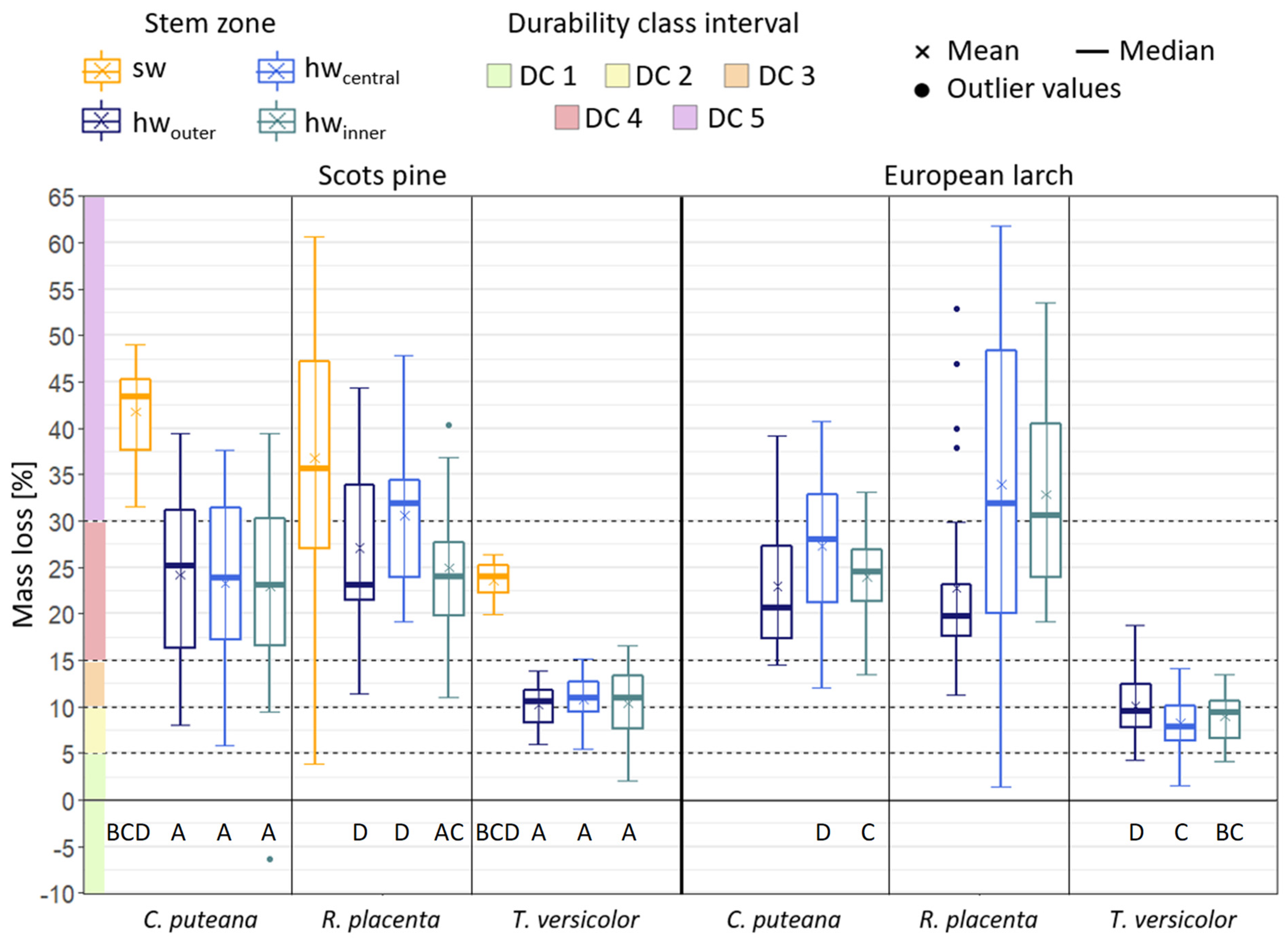
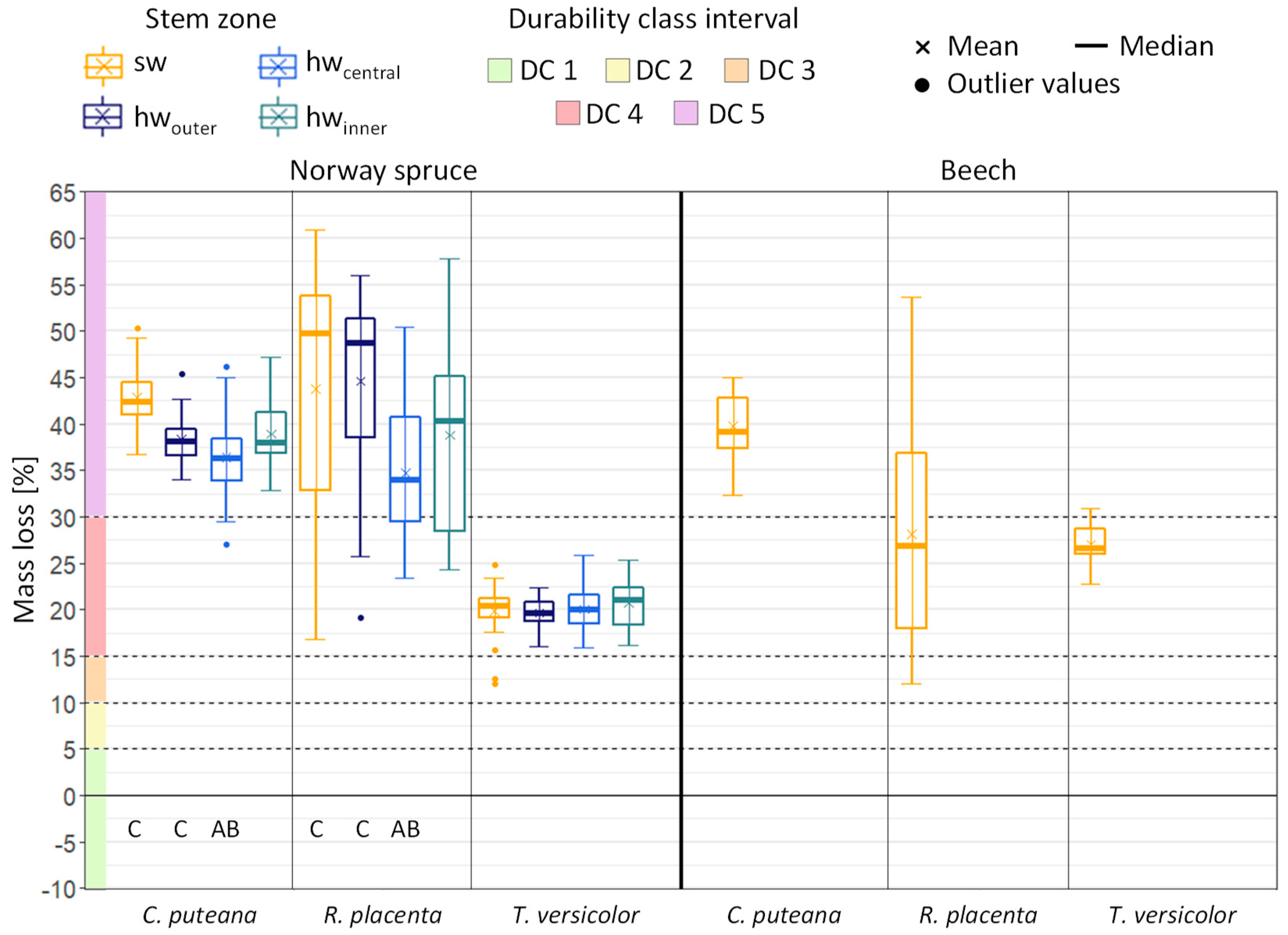
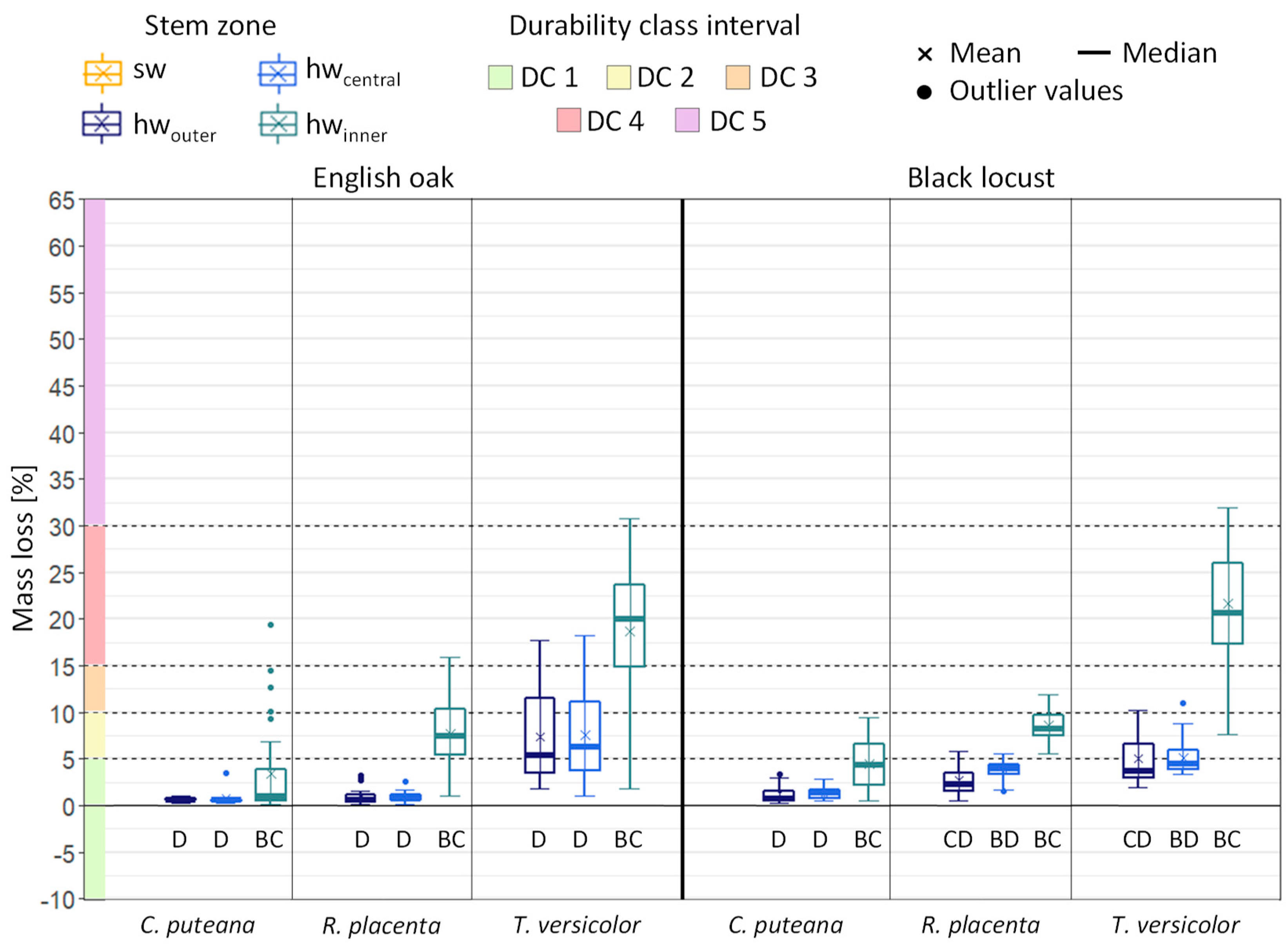
3.1. Mass Loss

Mass loss after 16 weeks of incubation with wood-destroying basidiomycetes differed between wood species, stem zones within one wood species, and test fungi (Figure 2, Figure 3 and Figure 4). All tests were valid since the ML thresholds of the virulence control specimens were passed by all three test fungi (i.e., 30% on Beech and Scots pine sapwood by C. puteana, 20% on Scots pine sapwood by R. placenta, and 20% on Beech by T. versicolor).

As expected, the sapwood of Scots pine showed significantly higher ML compared to the respective heartwood specimens (Figure 2), but the sapwood of Norway spruce showed similar ML compared to its heartwood (Figure 3). Furthermore, the juvenile wood (i.e., the inner heartwood) showed higher ML compared to the central and outer heartwood, in particular for Black locust and English oak (Figure 4), but not for the conifers, Scots pine, and European larch (Figure 2). Only small and in most cases, insignificant differences in ML were found between the outer and the central heartwood in all tested species (Figure 2, Figure 3 and Figure 4).

The white rot fungus T. versicolor caused higher ML on the hardwoods compared to the two brown rot fungi C. puteana and R. placenta, and the latter ones caused higher ML on the conifers with one exception; C. puteana caused the highest ML on Beech as previously reported by other authors [16,17].

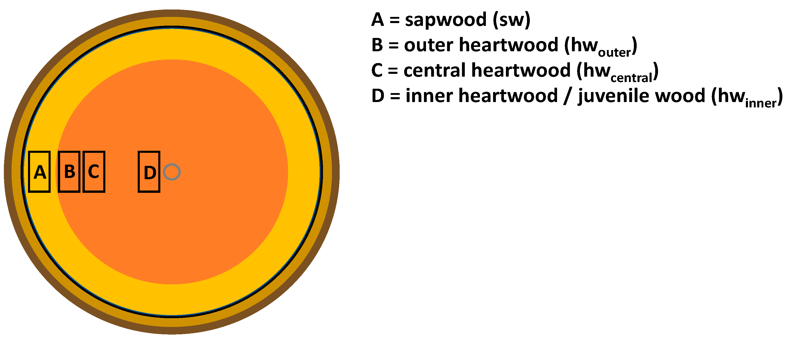
3.2. Sampling from Different Stem Zones

This study focused on the variability of the biological durability of untreated timbers. Hence, different stem zones were sampled separately. As shown above, the stem zone can have a major impact on ML data and, thus, on the resulting DCs. However, the precise sampling procedure undertaken in this study is rather unusual and often not possible, especially when boards or planks, but not logs, are sampled. Both standards, EN 350 [6] and EN 113-2 [9], suggest different sampling procedures for logs, sawn timber, and wood-based materials, where only the sampling of logs has a strong emphasis placed on stem zone differentiation. In contrast, for a sampling of sawn wood, the differentiation of stem zones is optional but can be discarded for a sampling of wood-based materials. According to EN 350 [6] sampling of logs shall separately consider sapwood, heartwood, and juvenile wood. For heartwood sampling, both the inner and the outer parts of the heartwood shall be incorporated, but juvenile wood, i.e., the region located 3 cm around the pith, shall be excluded. In general, the findings from this study support the guidance given by EN 350 [6], since only sapwood and juvenile wood showed a durability that significantly deviated from that of the remaining heartwood (Figure 2, Figure 3 and Figure 4). The differences between outer and central heartwood were negligibly small.

From a practical point of view, using different sampling procedures for logs, sawn timber, and wood-based materials appears reasonable but does not inevitably lead to the same DCs. For example, since juvenile wood in coloured heartwood can often not be distinguished from mature heartwood (e.g., Black locust) and since sapwood and non-coloured heartwood (e.g., Norway spruce) cannot be distinguished from each other, sampling from boards or planks cannot fulfil the above-mentioned requirements.

3.3. Applying Fitted Probability Density Functions to Mass Loss Data

According to EN 350 (2016), the proposed durability classification determined by the highest median ML “can be incorrect if high variability in results is present”. Therefore, the standard offers the option to express the spread of individual values based on fitted probability functions but does not suggest specific distributions that shall be used. EN 113-2 [9] refers to the procedure recommended by EN 350 [6] but adds that an “optional result analysis can be included: test for normality […] and fitting 3P Weibull-function to provide multiple parameters to assess the distribution.” In the standard [9], only Normal and Weibull distributions are proposed. However, some data sets showed the best fit using other types of distribution such as Gamma, Cauchy, and Log-normal distributions. Logarithmic and Exponential distributions were not found.

3.3.1. Handling Negative Mass Loss Values

The more durable a wood-based material is, the more likely the occurrence of negative ML data. Negative ML can be the result of erroneous mass measurements or the effect of ingrown fungal mycelium, as previously described by Meyer et al. [14]. Since some of the potential types of distributions solely operate with positive values (including Weibull), the following options to operate with negative ML values were evaluated:

(1)

The substitution of negative ML values by very small, but still positive operating values of 0.1e⁻¹⁰% does not lead to significant changes in the data set’s median value, which is crucial since the latter defines the DC. However, the mean value and the standard deviation are influenced by substituting negative values. Nevertheless, these values are parameter estimators for the fitting of affected distributions. An unspecific shift of these values due to substitution cannot be seen as a valid procedure, because this shift directly influences the calculation of the fitted probability function.

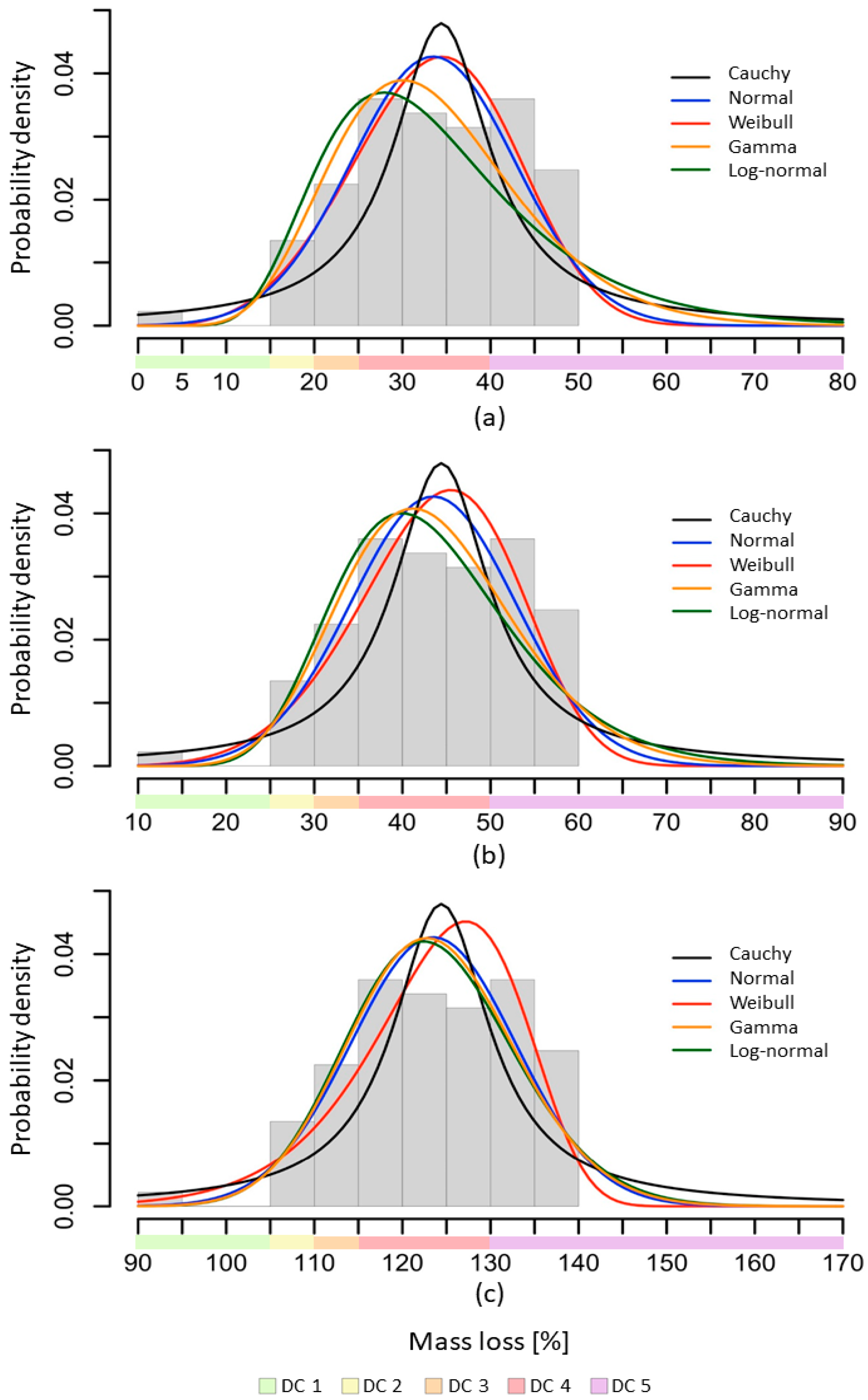
(2)

A low (10%), medium (20%), and high (100%) data translation along the x-axis was exemplarily performed for the ML data (hw_total) of Scots pine incubated with C. puteana. As shown in Figure 5, the data translation led to changes in the overall appearance of the fitted distributions; especially for Weibull, Gamma, and Log-normal distributions. The latter does not equally continue to ± ∞, but is limited to zero. Since the transformation of the fitted probability density function to the DC distribution is performed via the calculation of the integral area of the graph within the DC intervals, any compression or shift of the graph can lead to a non-transparent impact on the integral proportion within the DC intervals. The restriction of certain distributions to 0 (0 to +∞) in comparison to distributions with no limitation (−∞ to +∞) can cause non-transparent differences in the integral area per DC interval. Once the ML data analysis is completed, a reconstruction of empirical or fitted ML data via the integral percentage is impossible.

Data translation along the x-axis can cause shifts in the distribution curve. Without a consistent protocol for data translation, the resulting changes in the integral areas are neither comparable nor reconstructable—they can vary according to the individually chosen data translation technique. The effects of data translation may therefore lead to incomprehensible DC distribution, as the percental integral area per DC can be affected.

The portfolio of potential distribution types for data processing is limited without a clearly described procedure for transforming negative ML data. As a consequence, the comparability with other data sets containing solely positive values is constrained.

3.3.2. Data Fitting

Data fitting included a primary test for Normal distribution (Shapiro-Wilk). In this study, 40 of 69 data sets were normally distributed (

Table 3. Individual results of the Shapiro-Wilk test for normality. Number of replicates for sapwood (sw), outer heartwood (hw_outer), central heartwood (hw_central), inner heartwood (hw_inner): n = 30; Number of replicates for the total heartwood (hw_total): n = 90.

Wood Species	Test Fungi	Stem Zone
		sw	hwouter	hwcentral	hwinner	hwtotal
European larch	C. puteana	n.a.	*	-	-	-
	R. placenta	n.a.	***	-	**	***
	T. versicolor	n.a.	-	-	-	-
Norway spruce	C. puteana	-	-	-	-	-
	R. placenta	**	**	-	*	**
	T. versicolor	***	-	-	-	-
Scots pine	C. puteana	*	-	-	-	*
	R. placenta	-	*	-	-	**
	T. versicolor	-	-	-	-	-
European beech	C. puteana	-	n.a.	n.a.	n.a.	n.a.
	R. placenta	*	n.a.	n.a.	n.a.	n.a.
	T. versicolor	-	n.a.	n.a.	n.a.	n.a.
English oak	C. puteana	n.a.	-	***	***	***
	R. placenta	n.a.	***	**	-	***
	T. versicolor	n.a.	**	-	-	***
Black locust	C. puteana	n.a.	***	-	-	***
	R. placenta	n.a.	**	-	-	***
	T. versicolor	n.a.	***	***	-	***

Significance code: *** = most significant (p ≤ 0.001); ** = highly significant (p ≤ 0.01); * = significant (p ≤ 0.05); - = not significant (p > 0.05); n.a. = not available.

). Even though 32 of those 40 showed an even better fit with other types of distribution. This phenomenon is quite common and lies within the acceptable uncertainty of statistical testing. In general, a non-significant p-value for a standard test for Normal distribution can be seen as a valid reason to choose the Normal distribution as a base for the fitted probability density function approach. However, the follow-up best-fit analysis leads to a more reliable evaluation of the data distribution.

In addition to statistical testing, visual data assessment can be used to determine a reliable distribution. Figure 6 shows the histogram and fitted probability density function curves for a data set that was tested to be normally distributed via the Shapiro-Wilk test and best-fit analysis. In visual assessment, however, the Cauchy distribution was determined to be the most reliable. The human assessor concluded that while the Cauchy distribution underestimates several lower ML values, the histogram classes with the highest probability were more accurately represented, while the Normal distribution drastically underestimated the main represented histogram classes.

EN 350 [6] does not specify the selection process for the most suitable (best fit) probability density function, which bears the risk of producing deviating durability classifications even if the same ML data are used as a basis.

This effect can be amplified by the fact that differences in data fitting and resulting integral areas affect certain DCs more than others. DC 2 and DC 3 represent a ML interval range of 5%, which is clearly smaller than the range covered by DC 4 (15%), DC 1, and DC 5 (theoretically infinitive range). The smaller the DC’s ML range, the stronger the effect of data processing and fitting. Therefore, the proportions of DC 2 and DC 3 are most sensitive to dissimilar data processing.

For this study, all data fittings were based on the results of the best-fit analysis for the mentioned portfolio of distributions; if negative ML values occurred, the data set was only tested for distributions that were suitable for negative values.

3.4. Durability Classification

The median ML was used to determine the DC, and the empirical distribution of the ML data was used to define the different dispersion indicators (“x–y”, “x–z”, or “v”). Additionally, the percentage of the integral of the fitted probability density functions prorated to each DC interval was created and equally used to determine resulting dispersion indicators. The results for the examined soft- and hardwood species are shown in Table 3,

Table 4. Median mass loss (ML) of Scots pine specimens after incubation with different test fungi (C.p. = Coniophora puteana, R.p. = Rhodonia placenta, T.v. = Trametes versicolor), resulting durability classes (DC) according to EN 350 [6] and EN 113-2 [9] based on their empirical distribution and a distribution using a probability density function of best fit. DC based on fungus causing highest ML in bold. Discrepancies in DC are marked grey.

					Empirical Distribution **						Best Fit Density Function ***
Wood Species	Stem Zone	Test Fungus	Median ML [%]	DC *	DC 1 [%]	DC 2 [%]	DC 3 [%]	DC 4 [%]	DC 5 [%]	DC	DC 1 [%]	DC 2 [%]	DC 3 [%]	DC 4 [%]	DC 5 [%]	DC
Scots pine	sw	C.p.	43.4	5	-	-	-	-	100.0	5	-	-	-	1.2	98.8	5 2
		R.p.	35.7	5	3.3	-	-	33.3	63.3	5	0.6	1.2	2.6	25.4	70.2	5 1
		T.v.	24.1	4	-	-	-	100.0	-	4	-	-	0.1	99.9	-	4 2
	hwouter	C.p.	25.2	4	-	3.3	10.0	53.3	33.3	4	0.3	3.1	9.5	62.9	24.2	4 2
		R.p.	23.1	4	-	-	3.3	60.0	36.7	4	0.2	2.0	6.3	53.9	37.6	4 4
		T.v.	10.7	3	-	4.0	60.0	-	-	2–3	1.3	41.9	56.3	0.5	-	2–3 2
	hwcentral	C.p.	23.9	4	-	13.3	10.0	50.0	26.7	4v	1.1	5.9	12.6	56.7	23.7	4 2
		R.p.	31.9	5	-	-	-	36.7	63.3	5	-	0.5	2.4	42.8	54.3	4–5 3
		T.v.	10.7	3	-	40.0	60.0	-	-	2–3	1.3	41.9	56.3	0.5	-	2–3 2
	hwinner	C.p.	23.2	4	3.4	3.4	13.8	48.3	31.1	4	0.9	5.3	12.1	58.2	23.5	4 2
		R.p.	24.1	4	-	-	3.3	73.3	23.3	4	0.1	1.7	6.8	66.9	24.5	4 3
		T.v.	10.9	3	10.0	30.0	50.0	10.0	-	3v	8.6	37.8	41.8	11.8	-	3 1
	hwtotal	C.p.	23.7	4	1.1	6.7	11.2	50.6	30.4	4	1.7	5.3	10.2	55.4	27.4	4 2
		R.p.	25.2	4	-	-	2.2	56.7	41.1	4–5	-	0.2	3.2	61.9	34.7	4 3
		T.v.	10.8	3	3.3	35.6	56.7	4.4	-	3	3.2	39.9	51.8	5.1	-	3 2

* DC based on median mass loss, ** DC based on empirical distribution, *** DC based on best fit density function, ¹ Normal distribution, ² Weibull distribution, ³ Gamma distribution, ⁴ Log-normal distribution, ⁵ Cauchy distribution.

,

Table 5. Median mass loss (ML) of European larch specimens after incubation with different test fungi (C.p. = Coniophora puteana, R.p. = Rhodonia placenta, T.v. = Trametes versicolor), resulting durability classes (DC) according to EN 350 [6] and EN 113-2 [9] based on their empirical distribution and a distribution using a probability density function of best fit. DC based on fungus causing highest ML in bold. Discrepancies in DC are marked grey.

					Empirical Distribution **						Best Fit Density Function ***
Wood Species	Stem Zone	Test Fungus	Median ML [%]	DC *	DC 1 [%]	DC 2 [%]	DC 3 [%]	DC 4 [%]	DC 5 [%]	DC	DC 1 [%]	DC 2 [%]	DC 3 [%]	DC 4 [%]	DC 5 [%]	DC
European larch	hwouter	C.p.	20.7	4	-	-	3.3	76.7	20.0	4	-	0.2	8.2	78.0	13.6	4 4
		R.p.	19.7	4	-	-	13.3	73.3	13.3	4	-	2.1	15.5	65.5	17.0	3–5 4
		T.v.	9.6	2	10.0	43.3	33.3	13.3	-	2v	5.5	48.1	36.2	10.2	-	2v 3
	hwcentral	C.p.	28.0	4	-	-	10.0	46.7	43.3	4–5	0.1	1.1	4.7	56.4	37.7	4 2
		R.p.	32.0	5	6.6	-	-	36.7	56.7	5	4.3	3.5	5.3	27.7	59.2	5 1
		T.v.	7.9	2	13.3	60.0	26.7	-	-	2	15.2	55.5	27.4	1.9	-	1–3 2
	hwinner	C.p.	24.5	4	-	-	3.3	93.4	3.3	4	-	0.2	2.5	91.3	6.0	4 2
		R.p.	30.6	5	-	-	-	46.7	53.3	4–5	-	-	1.4	44.5	54.1	4–5 4
		T.v.	9.4	2	3.3	63.3	33.3	-	-	2	5.8	59.4	34.4	0.4	-	2 2
	hwtotal	C.p.	24.5	4	-	-	5.6	72.2	22.2	4	-	0.3	5.4	73.6	20.7	4 3
		R.p.	24.8	4	2.2	-	4.4	52.2	41.1	4–5	1.4	5.0	8.7	38.8	46.1	4 2
		T.v.	9.3	2	8.9	55.6	31.1	4.4	-	2	10.7	50.3	35.1	3.9	-	2 2

* DC based on median mass loss, ** DC based on empirical distribution, *** DC based on best fit density function, ¹ Normal distribution, ² Weibull distribution, ³ Gamma distribution, ⁴ Log-normal distribution, ⁵ Cauchy distribution.

,

Table 6. Median mass loss (ML) of Norway spruce specimens after incubation with different test fungi (C.p. = Coniophora puteana, R.p. = Rhodonia placenta, T.v. = Trametes versicolor), resulting durability classes (DC) according to EN 350 [6] and EN 113-2 [9] based on their empirical distribution and a distribution using a probability density function of best fit. DC based on fungus causing highest ML in bold.

					Empirical Distribution **						Best Fit Density Function ***
Wood Species	Stem Zone	Test Fungus	Median ML [%]	DC *	DC 1 [%]	DC 2 [%]	DC 3 [%]	DC 4 [%]	DC 5 [%]	DC	DC 1 [%]	DC 2 [%]	DC 3 [%]	DC 4 [%]	DC 5 [%]	DC
Norway spruce	sw	C.p.	42.4	5	-	-	-	-	100.0	5	-	-	-	-	100.0	5 4
		R.p.	49.8	5	-	-	-	13.3	86.7	5	-	0.1	0.5	11.3	88.1	5 2
		T.v.	20.5	4	-	-	6.7	93.3	-	4	-	0.8	2.3	92.2	2.9	4 5
	hwouter	C.p.	38.1	5	-	-	-	-	100.0	5	-	-	-	-	100.0	5 4
		R.p.	48.7	5	-	-	-	6.7	93.3	5	-	-	-	4.3	95.7	5 2
		T.v.	19.7	4	-	-	-	100.0	-	4	-	-	0.1	99.9	-	4 1
	hwcentral	C.p.	36.3	5	-	-	-	6.7	93.3	5	-	-	-	5.8	94.2	5 3
		R.p.	34.0	5	-	-	-	36.7	63.3	5	-	-	-	27.7	72.3	5 4
		T.v.	20.1	4	-	-	-	100.0	-	4	-	-	0.3	99.7	-	4 4
	hwinner	C.p.	38.1	5	-	-	-	-	100.0	5	-	-	-	0.1	99.9	5 4
		R.p.	40.3	5	-	-	-	33.3	66.7	5	-	-	0.1	18.4	81.5	5 3
		T.v.	21.1	4	-	-	-	100.0	-	4	-	-	1.5	98.5	-	4 1
	hwtotal	C.p.	37.6	5	-	-	-	2.2	97.8	5	-	-	-	1.2	98.8	5 1
		R.p.	40.0	5	-	-	-	25.8	74.2	5	-	0.1	0.6	16.0	83.3	5 2
		T.v.	19.9	4	-	-	-	100.0	-	4	-	-	0.4	99.6	-	4 4

* DC based on median mass loss, ** DC based on empirical distribution, *** DC based on best fit density function, ¹ Normal distribution, ² Weibull distribution, ³ Gamma distribution, ⁴ Log-normal distribution, ⁵ Cauchy distribution.

,

Table 7. Median mass loss (ML) of English oak specimens after incubation with different test fungi (C.p. = Coniophora puteana, R.p. = Rhodonia placenta, T.v. = Trametes versicolor), resulting durability classes (DC) according to EN 350 [6] and EN 113-2 [9] based on their empirical distribution and a distribution using a probability density function of best fit. DC based on fungus causing highest ML in bold. Discrepancies in DC are marked grey.

					Empirical Distribution **						Best Fit Density Function ***
Wood Species	Stem Zone	Test Fungus	Median ML [%]	DC *	DC 1 [%]	DC 2 [%]	DC 3 [%]	DC 4 [%]	DC 5 [%]	DC	DC 1 [%]	DC 2 [%]	DC 3 [%]	DC 4 [%]	DC 5 [%]	DC
English oak	hwouter	C.p.	0.7	1	100.0	-	-	-	-	1	99.3	0.4	0.1	0.1	0.1	1 5
		R.p.	0.7	1	100.0	-	-	-	-	1	99.3	0.6	0.1	-	-	1 4
		T.v.	5.4	2	46.7	26.7	13.3	13.3	-	2v	40.9	37.1	13.3	7.8	0.9	2 4
	hwcentral	C.p.	0.6	1	100.0	-	-	-	-	1	99.3	0.4	0.1	0.1	0.1	1 4
		R.p.	0.8	1	100.0	-	-	-	-	1	100.0	-	-	-	-	1 4
		T.v.	6.4	2	36.7	30.0	26.7	6.7	-	1–3	34.2	39.0	19.2	7.6	-	1–3 2
	hwinner	C.p.	1.0	1	76.7	10.0	10.0	3.3	-	1v	83.3	10.0	3.2	2.6	0.9	1 4
		R.p.	7.5	2	23.3	50.0	23.3	6.7	-	1–3	24.5	49.4	22.6	3.5	-	1–3 2
		T.v.	20.1	4	3.3	13.3	10.0	70.0	3.3	4v	2.4	8.0	19.2	65.3	5.1	4 1
	hwtotal	C.p.	0.7	1	92.2	3.3	3.3	1.1	-	1	99.0	0.5	0.2	0.2	0.1	1 5
		R.p.	1.2	1	74.4	16.7	7.8	1.1	-	1	83.0	10.5	3.2	2.5	0.8	1 4
		T.v.	9.7	2	28.9	23.3	16.7	30.0	1.1	1–4/2v	23.3	28.5	21.5	24.1	2.6	1–4/2v 2

* DC based on median mass loss, ** DC based on empirical distribution, *** DC based on best fit density function, ¹ Normal distribution, ² Weibull distribution, ³ Gamma distribution, ⁴ Log-normal distribution, ⁵ Cauchy distribution.

,

Table 8. Median mass loss (ML) of Black locust specimens after incubation with different test fungi (C.p. = Coniophora puteana, R.p. = Rhodonia placenta, T.v. = Trametes versicolor), resulting durability classes (DC) according to EN 350 [6] and EN 113-2 [9] based on their empirical distribution and a distribution using a probability density function of best fit. DC based on fungus causing highest ML in bold. Discrepancies in DC marked grey.

					Empirical Distribution **						Best Fit Density Function ***
Wood Species	Stem Zone	Test Fungus	Median ML [%]	DC *	DC 1 [%]	DC 2 [%]	DC 3 [%]	DC 4 [%]	DC 5 [%]	DC	DC 1 [%]	DC 2 [%]	DC 3 [%]	DC 4 [%]	DC 5 [%]	DC
Black locust	hwouter	C.p.	0.8	1	100.0	-	-	-	-	1	99.1	0.9	-	-	-	1 4
		R.p.	2.3	1	86.7	13.3	-	-	-	1	92.1	7.6	0.3	-	-	1 4
		T.v.	3.8	1	63.3	30.0	6.7	-	-	1	59.8	34.6	4.7	0.9	-	1 4
	hwcentral	C.p.	1.4	1	100.0	-	-	-	-	1	100.0	-	-	-	-	1 3
		R.p.	4.0	1	83.3	16.7	-	-	-	1	89.5	10.5	-	-	-	1 2
		T.v.	4.5	1	63.3	33.3	3.3	6.7	-	1	52.5	46.8	0.7	-	-	1–2 4
	hwinner	C.p.	4.4	1	63.3	36.7	-	-	-	1	63.1	33.2	3.6	0.1	-	1 2
		R.p.	8.2	2	-	76.7	23.3	-	-	2	0.8	78.5	20.6	0.1	-	2 3
		T.v.	20.7	4	-	3.3	-	90.0	6.7	4	0.1	1.8	9.6	83.0	5.5	4 2
	hwtotal	C.p.	1.5	1	87.8	12.2	-	-	-	1	90.4	7.8	1.3	0.5	-	1 4
		R.p.	4.2	1	56.7	35.5	7.8	-	-	1	57.5	35.4	6.2	0.9	-	1 3
		T.v.	6.3	2	42.2	22.2	3.4	30.0	2.2	1–4/2v	29.7	33.2	16.9	15.7	4.5	1–4/2v 4

* DC based on median mass loss, ** DC based on empirical distribution, *** DC based on best fit density function, ¹ Normal distribution, ² Weibull distribution, ³ Gamma distribution, ⁴ Log-normal distribution, ⁵ Cauchy distribution.

and

Table 9. Median mass loss (ML) of Beech specimens after incubation with different test fungi (C.p. = Coniophora puteana, R.p. = Rhodonia placenta, T.v. = Trametes versicolor), resulting durability classes (DC) according to EN 350 [6] and EN 113-2 [9] based on their empirical distribution and a distribution using a probability density function of best fit. DC based on fungus causing highest ML in bold. Discrepancies in DC marked grey.

					Empirical Distribution **						Best Fit Density Function ***
Wood Species	Stem Zone	Test Fungus	Median ML [%]	DC *	DC 1 [%]	DC 2 [%]	DC 3 [%]	DC 4 [%]	DC 5 [%]	DC	DC 1 [%]	DC 2 [%]	DC 3 [%]	DC 4 [%]	DC 5 [%]	DC
Beech	sw	C.p.	39.2	5	-	-	-	-	100.0	5	-	-	-	-	100.0	5 1
		R.p.	26.9	4	-	-	10.0	43.3	46.7	4–5	-	1.6	7.6	52.6	38.2	4 3
		T.v.	26.7	4	-	-	-	93.3	6.7	4	-	-	-	92.6	7.4	4 1

* DC based on median mass loss, ** DC based on empirical distribution, *** DC based on best fit density function, ¹ Normal distribution, ² Weibull distribution, ³ Gamma distribution, ⁴ Log-normal distribution, ⁵ Cauchy distribution.

.

With a sample size of 30 specimens, each specimen accounts for 3.3% of the empirical DC distribution. While ML is a continuous variable, the empirical DC distribution only allows discrete steps based on the sample size—this holds true, despite decimal digit and percentage numbers suggesting otherwise. Using fitted probability density functions seems to be an attempt to transform the discrete empirical DC distribution into a continual theoretical distribution. The effect is distinctly recognisable for boundary values and DCs that only hold 1–3 specimens (3.3–9.9%) in the empirical DC distribution.

The effect of fitting the data to probability density functions can be seen in Table 3, Table 4, Table 5, Table 6, Table 7 and Table 8. For instance, while Scots pine heartwood (hw_total) is assigned to DC 4 based on the median ML by R. placenta, it is DC 4–5 based on the empirical distribution, and DC 4 based on the best fit density function (Table 3). As intended, the distribution of the DCs provides information about the variability in durability, and the latter can be expressed through dispersion indicators, either in the form of DC ranges (‘x-y’ or ‘x-z’) or by the supplement ‘v = variable’. In summary, fitting the ML data to a probability density function led in two cases to a higher DC or DC range, respectively, and in one case to a lower DC, but had no effect in 14 cases (Table 3, Table 4, Table 5 and Table 6). More difficult to interpret is the addition of the dispersion indicator ‘v’ since, per definition, it does not provide any quantitative information about the spread of DC as the following example illustrates: The outer heartwood (hw_outer) of English oak is assigned to DC 2v and the inner heartwood (hw_inner) to DC 4v, both based on the empirical distribution of ML data referring to T. versicolor (Table 6). The outer heartwood included more ML data referring to higher durability, i.e., DC 1, compared to those referring to lower durability, i.e., DC 3 and 4 together. In contrast, hw_inner included more than 10% ML data referring to DC 3 and 4, respectively, but less than 10% in DC 5. Consequently, the supplement ‘v’ only indicates that a certain spread exists but does not inform about its quality.

In two cases, i.e., the hw_total of English oak and Black locust, more than one dispersion indicator could be assigned. The distribution of ML data fulfilled both the requirements for the range DC 1–4 and the supplement ‘v’, which, combined with the median-based classification, led to DC 2v. Again, the indicator ‘v’ did not inform about the qualitative spread, while the indication of a range did not inform about the quantitative spread. The latter became particularly evident for Black locust heartwood, which contained between 22 and 42% ML data in DC 1, 2, and 4, but only 3.4% in DC 3.

3.5. Further Aspects under Debate

In addition to the questions examined in this study, there are a number of other aspects that have been discussed controversially for some time in the context of the durability testing of wood in the laboratory. These include the aspects summarized below.

In the agar-plate test for determining the durability of wood against wood-destroying fungi the most common measure is ML by fungal attack, which can be expressed absolutely in grams or as a percentage of the initial oven-dry mass [18]. The absolute ML is a measure of fungal activity (how much wood substance the fungus was able to metabolize), i.e., a measure of decay susceptibility. In contrast, the percentage ML is a measure of the remaining wood substance or the remaining strength of the material [19], and thus a measure of wood durability. When comparing the resistance of wood-based materials of different densities the absolute ML should be considered. However, it has been frequently recommended to use the percentage ML for durability classification [18] even if wood blocks vary in density. Nevertheless, it is commonly accepted that the specimen volume as well as the incubation must not be changed at a given schedule for the assignment of durability classes, e.g., according to EN 113-2 [9] and EN 350 [6]. To become furthermore independent from the virulence of the test fungi, relative percentage ML can be used as, for instance, required for soft rot resistance tests according to CEN/TS 15083-2 [7] and graveyard field tests according to EN 252 [8] in form of so-called ‘x-values’.

According to EN 113-2 [9], test specimens need to get sterilized before incubation using either gamma radiation or steam treatment. The latter shall only be used for materials that are heat-resistant and not volatile at high temperatures. However, since, in case of doubt, it is not known at all how the material or the treatment agent behaves, it may be questioned whether this sterilisation method can be used optionally. In contrast, gamma radiation can affect the structural integrity of the wood and its chemical constitution as well [20] and it cannot be excluded that it also influences the results of the durability test [21]. More recently, different sterilization methods as well as the effect of oven-drying for ML measurements of the test specimens on the resulting durability were examined by Brischke et al. [22]. They found no significant ML differences between sterilization through gamma radiation, steam, autoclaving, ethanol dipping, and oven-drying. Solely, non-sterilized specimens showed a reduced ML, since the test fungus was inhibited by mould growth. Oven-drying of wood species that contain volatile and resistance-affecting compounds such as Scots pine (Pinus sylvestris) led to reduced biological durability and should either be avoided or adapted to kiln-drying temperatures above 60 °C as usually applied in practice.

The incubation time in durability agar plate tests is fixed, for instance, 16 weeks according to EN 113-2 [9]. However, it has been repeatedly suggested that prolonged incubation times may be necessary to allow for fungal attack which can be delayed through cell wall modification or biocidal treatments [23,24,25]. However, it does not seem advisable to deviate from the specified incubation period for the following reasons: (1) malt agar serves as a source of nutrients and moisture, but dries out when the incubation time significantly exceeds 16 weeks. Adding water during the running experiment is challenging since the agar does not take up water after it has gelled; (2) the comparability of test results is limited since keeping specimen size and the incubation time constant is the basis for durability classification according to EN 113-2 [9]. The assumption that prolonged incubation times can prevent negative ML from occurring cannot be confirmed either. Negative ML is a common phenomenon when testing very durable but non-toxic materials, i.e., the test fungus is not able to degrade the wood, but can easily colonize it [26,27] and will not change in elongated tests.

4. Conclusions

The biological durability of six different European-grown wood species has been tested against different wood-destroying fungi according to the European standards EN 350 [6] and EN 113-2 [9]. The spread of the obtained mass loss (ML) data has been extensively and comparatively analysed using different statistical methods. The following can be concluded from the results of the analysis:

• Since the durability can vary not only between sapwood, heartwood, and juvenile wood but also between outer and central heartwood, more precise guidance is needed on the sampling procedure. Especially when sampling boards, planks, and wood products, it is difficult to differentiate between stem zones which are not adequately addressed by the current standards.
• Showing the spread of individual ML data using fitted probability density functions is an optional but recommended element of the test protocol according to EN 113-2 [9]. However, the proposed statistical treatment is inadequately described and thus hardly reproducible. In particular, the standard lacks a description of the selection procedure of the best-fitting density function.
• The application of probability density functions is demanding and laborious. The comparison of DCs based on empirical distributions and those derived from best-fitted density functions showed that only marginal differences could be expected. The additional information about the variability of wood durability is rather limited. Furthermore, the statistical procedure is highly complex, and its application may cause further sources of error.
• Generally, the assignment of dispersion indicators appeared meaningful since it could provide additional information about the variability of wood durability. However, using two different and non-complementary indicators may cause confusion. Preference should be given to indicators that provide both qualitative and quantitative information. A range of DCs should take precedence over the variability index ‘v’.

References

1. Van Acker, J.; Stevens, M.; Carey, J.; Sierra-Alvarez, R.; Militz, H.; Le Bayon, I.; Kleist, G.; Peek, R.D. Biological durability of wood in relation to end-use. Holz als Roh- und Werkstoff. 2003, 61, 35–45. [Google Scholar] [CrossRef]
2. Augusta, U. Untersuchung der Natürlichen Dauerhaftigkeit Wirtschaftlich Bedeutender Holzarten bei Verschiedener Beanspruchung im Außenbereich. Ph.D. Thesis, University of Hamburg, Hamburg, Germany, 2007. [Google Scholar]
3. Brischke, C.; Alfredsen, G.; Humar, M.; Conti, E.; Cookson, L.; Emmerich, E.; Flæte, P.O.; Fortino, S.; Francis, L.; Hundhausen, U.; et al. Modelling the material resistance of wood—Part 2: Validation and Optimization of the Meyer-Veltrup Model. Forests 2021, 12, 590. [Google Scholar] [CrossRef]
4. Brischke, C.; Alfredsen, G.; Humar, M.; Conti, E.; Cookson, L.; Emmerich, E.; Flæte, P.O.; Fortino, S.; Francis, L.; Hundhausen, U.; et al. Modelling the material resistance of wood—Part 3: Relative resistance in above and in ground situations—Results of a global survey. Forests 2021, 12, 576. [Google Scholar] [CrossRef]
5. Brischke, C.; Alfredsen, G. Biological durability of pine wood. Wood Mat. Sci. Eng. 2022, 18, 1050–1064. [Google Scholar] [CrossRef]
6. EN 350; Durability of Wood and Wood-Based Products—Testing and Classification of the Durability to Biological Agents of Wood and Wood-Based Materials. European Committee for Standardization: Brussels, Belgium, 2016.
7. CEN/TS 15083-2; Durability of Wood and Wood-Based Products—Determination of the Natural Durability of Solid Wood against Wood-Destroying Fungi, Test. Methods—Part 2: Soft Rotting Micro-Fungi. European Committee for Standardization (CEN): Brussels, Belgium, 2005.
8. EN 252; Field Test Method for Determining the Relative Protective Effectiveness of a Wood Preservative in Ground Contact. European Committee for Standardization: Brussels, Belgium, 2015.
9. EN 113-2; Durability of Wood and Wood-Based Products—Test. Method against Wood Destroying Basidiomycetes—Part. 2: Assessment of Inherent or Enhanced Durability. European Committee for Standardization: Brussels, Belgium, 2021.
10. Van Acker, J.; Palanti, S. Durability. In Performance of Bio-Based Building Materials; Jones, D., Brischke, C., Eds.; Elsevier: Duxford, UK, 2017; pp. 257–277. [Google Scholar]
11. Alfredsen, G.; Brischke, C.; Marais, B.N.; Stein, R.F.; Zimmer, K.; Humar, M. Modelling the material resistance of wood—Part 1: Utilizing durability test data based on different reference wood species. Forests 2021, 12, 558. [Google Scholar] [CrossRef]
12. Bollmus, S.; Bächle, L.; Militz, H.; Brischke, C. Durability classification of preservative treated and modified wood. In Proceedings of the IRG Annual Meeting, IRG/WP 19-20659, Quebec City, QC, Canada, 12–16 May 2019; p. 17. [Google Scholar]
13. Brischke, C.; Bollmus, S.; Melcher, E.; Stephan, I. Biological durability and moisture dynamics of Dawn redwood (Metasequoia glyptostroboides) and Port Orford cedar (Chamaecyparis lawsoniana). Wood Mat. Sci. Eng. 2022, 18, 1024–1034. [Google Scholar] [CrossRef]
14. Meyer, L.; Brischke, C.; Treu, A.; Larsson-Brelid, P. Critical moisture conditions for fungal decay of modified wood by basidiomycetes as detected by pile tests. Holzforschung 2016, 70, 331–339. [Google Scholar] [CrossRef]
15. R Core Team. R: A Language and Environment for Statistical Computing; R Foundation for Statistical Computing: Vienna, Austria, 2020; Available online: http://www.r-project.org/index.html (accessed on 11 April 2023).
16. Brischke, C.; Welzbacher, C.R.; Gellerich, A.; Bollmus, S.; Humar, M.; Plaschkies, K.; Scheiding, W.; Alfredsen, G.; Van Acker, J.; De Windt, I. Wood natural durability testing under laboratory conditions: Results from a round-robin test. Eur. J. Wood Wood Prod. 2014, 72, 129–133. [Google Scholar] [CrossRef]
17. Emmerich, L.; Ehrmann, A.; Brischke, C.; Militz, H. Comparative studies on the durability and moisture performance of wood modified with cyclic N-methylol and N-methyl compounds. Wood Sci. Technol. 2021, 55, 1531–1554. [Google Scholar] [CrossRef]
18. Nilsson, T.; Daniel, G. On the use of% weight loss as a measure for expressing results of laboratory decay experiments. In Proceedings of the IRG Annual Meeting, IRG/WP 92-2394, Harrogate, UK, 10–15 May 1992; p. 6. [Google Scholar]
19. Brischke, C.; Bayerbach, R.; Rapp, A.O. Decay-influencing factors: A basis for service life prediction of wood and wood-based products. Wood Mat. Sci. Eng. 2006, 1, 91–107. [Google Scholar] [CrossRef]
20. Despot, R.; Hasan, M.; Brischke, C.; Welzbacher, C.R.; Rapp, A.O. Changes in physical, mechanical and chemical properties of wood during sterilisation by gamma radiation. Holzforschung 2007, 61, 267–271. [Google Scholar] [CrossRef]
21. Despot, R.; Hasan, M.; Glavaš, M.; Rep, G. On the changes of natural durability of wood sterilised by gamma radiation. In Proceedings of the IRG Annual Meeting, IRG/WP 06-10571, Tromsø, Norway, 18–22 June 2006; p. 12. [Google Scholar]
22. Brischke, C.; von Boch-Galhau, N.; Bollmus, S. Impact of different sterilization techniques and mass loss measurements on the durability of wood against wood-destroying fungi. Eur. J. Wood Wood Prod. 2022, 80, 35–44. [Google Scholar] [CrossRef]
23. Donath, S.; Militz, H.; Mai, C. Creating water repellent effects on wood by treatment with silanes. Holzforschung 2006, 60, 40–46. [Google Scholar] [CrossRef]
24. Beck, G.; Thybring, E.E.; Thygesen, L.G. Brown-rot fungal degradation and de-acetylation of acetylated wood. Int. Biodeter. Biodegr. 2018, 135, 62–70. [Google Scholar] [CrossRef]
25. Thygesen, L.G.; Beck, G.; Nagy, N.E.; Alfredsen, G. Cell wall changes during brown rot degradation of furfurylated and acetylated wood. Int. Biodeter. Biodegr. 2021, 162, 105257. [Google Scholar] [CrossRef]
26. Brischke, C.; Soetbeer, A.; Meyer-Veltrup, L. The minimum moisture threshold for wood decay by basidiomycetes revisited. A review and modified pile experiments with Norway spruce and European beech decayed by Coniophora puteana and Trametes versicolor. Holzforschung 2017, 71, 893–903. [Google Scholar] [CrossRef]
27. Emmerich, L.; Bleckmann, M.; Strohbusch, S.; Brischke, C.; Bollmus, S.; Militz, H. Growth behavior of wood-destroying fungi in chemically modified wood: Wood degradation and translocation of nitrogen compounds. Holzforschung 2021, 75, 786–797. [Google Scholar] [CrossRef]
Figure 1. Stem sections sampled for durability tests.
Standards 03 00017 g001
Figure 2. Mass loss of Scots pine and European larch after 16 weeks of incubation with wood-destroying basidiomycetes differentiated by test fungi and stem zones. Values outside the 1.5 interquartile range were considered outliers. Number of replicates: n = 30. Capital letters indicate significant differences from other stem sections (p ≤ 0.05).
Standards 03 00017 g002
Figure 3. Mass loss of Norway spruce and Beech after 16 weeks of incubation with wood-destroying basidiomycetes differentiated by test fungi and stem zones. Values outside the 1.5 interquartile range were considered outliers. Number of replicates: n = 30. Capital letters indicate significant differences from other stem sections (p ≤ 0.05).
Standards 03 00017 g003
Figure 4. Mass loss of English oak and Black locust after 16 weeks of incubation with wood-destroying basidiomycetes differentiated by test fungi and stem zones. Values outside the 1.5 interquartile range were considered outliers. Number of replicates: n = 30. Capital letters indicate significant differences from other stem sections (p ≤ 0.05).
Standards 03 00017 g004
Figure 5. Data translation of the histogram along the x-axis and the resulting fitted probability density functions of different distributions for a parallel shift of (a) 10%, (b) 20%, and (c) 100% by taking the example of Scots pine heartwood ML after incubation with C. puteana (n = 89).
Standards 03 00017 g005
Figure 6. Histogram and fitted probability density function curves of mass loss of English oak after incubation with T. versicolor (n = 30). The data set was tested to be normally distributed via the Shapiro-Wilk test and best-fit analysis.
Standards 03 00017 g006