Article

Single Image Deblurring for Pulsed Laser Range-Gated Imaging System with Multi-Slice Integration

1
College of Weapons Engineering, Naval University of Engineering, Wuhan 430033, China
2
Naval Petty Officer School, Bengbu 233012, China
*
Author to whom correspondence should be addressed.
Photonics 2022, 9(9), 642; https://doi.org/10.3390/photonics9090642
Submission received: 9 August 2022 / Revised: 24 August 2022 / Accepted: 2 September 2022 / Published: 7 September 2022

Abstract

:
The multi-slice integration (MSI) method is one of the approachs to extend the depth of view (DOV) of the pulsed laser range-gated imaging (PLRGI) system. When the DOV is large enough and exceeds the depth of focus of the system, it may make some targets in the image clear and others blurred. In addition, forward scatter is also considered to have a blurring effect on the image. There is very little literature to solve the combined effect of forward scatter and defocus. An imaging model is built based on the model from Jaffe–McGlamery and Fourier optics. According to the imaging model, backscattered light is independent from reflected light from the target, and forward scatter has a relationship with the reflected light. Thus, backscattered light should be removed before deblurring. First, rolling ball and intensity transformation are used to remove the backscattered light and enhance the image. Then, a deep learning model based on Transformer is used to deblur the image. To enable the deep learning model to accommodate different degrees of blurred image, 16 different blur kernels are generated according to the imaging model. Sharp images from a DPDD dataset were chosen to train the model. Images of varying degrees of blur were collected from a water tank and a boat tank by the PLRGI system as test sets. Image deblurring results show that the proposed method can remove different levels of blur and can deal with images which have sharp targets and blurred targets together.

1. Introduction

Pulsed laser range-gated imaging (PLRGI) is one of the most effective methods to achieve underwater high-resolution imaging [1,2,3]. The conventional PLRGI system is mostly used for in situ observation for the limitation of the depth of view (DOV). To extend the DOV, many methods can be used. One is multi-channel receivers, which can acquire images from multi-slice at the same time [4,5]. However, this will make the system too complex and expensive. Another one is the multi-pulse integration (MPI) method, which splits the detection area into multi-areas and assigns pulses to detect each area alone and combines them to a single image [6,7]. Nevertheless, the number of pulses allocated to each slice is the same in the literature, and this makes it similar to a single slice with a large DOV. The MPI method introduces the problem that the distant target is much darker than the near target. Thus, we propose the multi-slice integration (MSI) method in the literature [8]. Different from the MPI method, the number of the pulses assigned to each slice and gate width (GW) of each slice can be different from each other in the MSI method. In this case, by adjusting the system parameters, the intensity of targets at different distances can be approximately equal. When the DOV is extended, the distance between multiple targets in the field of view may exceed the depth of focus (DOF), resulting in clear imaging of some targets and blurring of others (same as blur caused by improper focal length setting). In addition, forward scatter in water also has an effect on the blurring of the image [9]. Similar to other optical systems, the motion of the system or target can also cause image blur. Since motion blur is different from the above two blurring effects, it is not considered in this paper.
Forward scatter changes the direction of the light and blurs the image of the target. Various solutions have been proposed to address the blurring caused by the forward scatter. One is to build a model related to the shape and background of the target [10,11,12], and use the model to estimate the intensity and distribution of forward scattering light. The key point of these model-based methods is the accurate estimation of medium transmission [13,14,15]. However, these methods always are unstable and sensitive for three reasons: (1) image recovery is an ill-posed problem, (2) the underwater environment is complex and estimating underwater imaging parameters is difficult, and (3) underwater imaging models may be inaccurate in some cases. Another one is to deconvolve the blurred image using an iterative approach [9,16]. However, this approach relies on the initial estimate and has a high computational cost. There are also methods for underwater image enhancement which come with the ability to remove forward scatter [15,17]. However, they mainly focus on color cast, low contrast or backscattered light removal.
For defocus blur, researchers focus on detection and segmentation of the defocus blur area [18], defocus map estimation [19] and defocus blur removal. The traditional approach for defocus blur removal is to estimate the point spread function (PSF) and then use a deconvolution method to restore a clear image. However, the PSF is hard to estimate for the same reasons of model-based methods. In recent years, researchers have preferred to use deep learning methods to remove defocus blur. This approach uses an end-to-end network architecture that skips complex modeling problems and enables direct mapping of blurred images to clear images. Abuolaim [20] proposed DPDNet for removing defocus blur. However, the method is limited by the hardware, and the performance of the single image deblurring method needs to be improved. Son [21] proposed a kernel-sharing parallel atrous convolutional (KPAC) block for single image defocus deblurring. Quan [22] proposed a pixel-wise Gaussian kernel mixture deep neural network (GKMNet) for single image defocus blur removal. However, their performances on severely blurred regions is not that satisfactory. All the above networks are designed based on convolutional neural networks. Convolution is a local operation that usually only models the relationship between neighboring pixels. Transformer, on the other hand, is a global operation that models the relationship between all pixels. As a result, image restoration using Transformer is now at the forefront [23,24].
For underwater range-gated imaging, a blurred image is caused by the combined effect of forward scatter and defocus. Most of the literature focuses on removing the effects of forward scatter. There is very little literature to solve the combined effect of forward scatter and defocus blur due to the small DOV of the PLRGI system. In this paper, a two-step method is proposed to deblur the image collected by the PLRGI system with an MSI method. The main contributions of this paper are highlighted as follows.
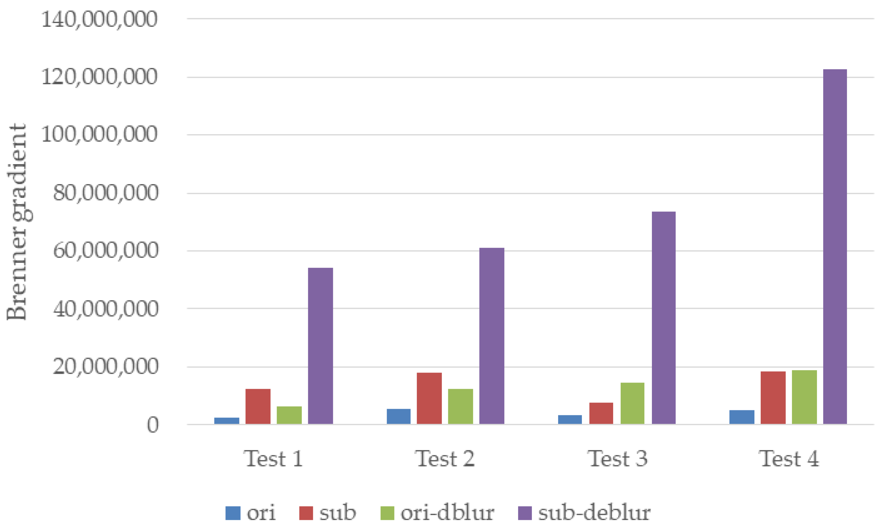
  • A two-step method is proposed to deblur the blurred image caused by the combined effect of forward scatter and defocus.
  • An imaging model is built to generate training data for the network, and this can enable the model to deal with different levels of blurred image. It makes use of merits of both knowledge of underwater imaging and deep neural networks.
  • Our method outperforms two state-of-the-art methods on several experiments under different water conditions in terms of both visual quality and quantitative metrics.
The paper is organized as follows: following this introduction section, principles of the MSI method are described, and an imaging model is built based on the model from Jaffe–McGlamery and Fourier optics. In Section 3, a two-step method is proposed to deblur the image according to the imaging model. First, rolling ball and intensity transformation are used to remove the backscattered light and enhance the image. Then, a deep learning model based on Transformer is used to deblur the image. In Section 4, in order to validate the method proposed, experiments were carried out to obtain the blurred image from the PLRGI system, and the experimental results are presented and discussed. Conclusions are drawn in the last section.

2. Theory

2.1. Multi-Slice Integration Method for PLRGI System

The PLRGI system enables a slice imaging approach similar to that of computed tomography. Position and width of the slice depends on the delay time and gate width. Intensity of the slice depends on the number of pulses assigned to the slice. To illustrate the principle of the MSI method, we take three slices, for example, which are shown in Figure 1. In the system, a laser with a high pulse repetition frequency is in use. The laser pulses in one video frame can be split into three groups, and each group corresponds to one slice. Each slice has its own delay time and gate width.
The timing sequence of the MSI method is shown in Figure 1b. The number of pulses assigned to target ①, ② and ③ are n1, n2 and n3, respectively. Delay time of three groups are t1, t2 and t3, which are different from each other. Every pulse has a range intensity profile (RIP), and pulses belonging to same group have the same RIP. Finally, three sub-RIPs are integrated in a frame and generate an image with an integrated RIP.
RIP of a single pulse can be expressed as,
E i ( z ) = ( 2 z c w t i + τ P ) Φ , 2 z c w [ τ p , 0 ] τ P Φ , 2 z c w [ 0 , τ i τ p ] ( τ i + t i 2 z c w ) Φ , 2 z c w [ τ i τ p , τ i ]
where τP is the pulse width, cw is speed of the laser in water, ti is the delay time of the gate, τi is gate width, z is the distance of the target, z′ = z-cwti/2, and Φ is the laser pulse radiant flux that reach the camera. More details about the integrated RIP can be obtained from the literature [8].
Integrated RIP in a frame is,
E i n t e g r a t e d = k = 1 3 n k E k
where k means kth slice, and Ek can be obtained from Equation (1).

2.2. Imaging Model Based on Jaffe-McGlamery

The commonly used underwater imaging model was developed by Jaffe [25] after improving on the model proposed by McGlamery [26]. According to the model, the total irradiance Etotal that reaches the sensor consists of three components: light reflected from the target, forward scattering light from the reflected light and backscattered light from water. Etotal can be expressed as,
E t o t a l = E t arg e t + E f s + E b s
Here Etarget equals Eintegrated for the MSI method. Efs and Ebs denote energy of forward scattering light and energy of backscattered light, respectively.
According to the Fourier optics, light energy output from CCD equals the convolution of Etotal and the modulation transfer function (MTF) of the receiver MTFsys and can be expressed as,
E o u t = E t o t a l F 1 ( MTF sys )
where F−1 is the inverse Fourier Transform.
From Equations (3) and (4), we can acquire,
E o u t = E t arg e t F 1 ( MTF sys ) + E f s F 1 ( MTF sys ) + E b s F 1 ( MTF sys )
For forward scattering light, Efs can be calculated by the convolution operation of reflected light and the PSF of water. There are many models for the PSF of water. Here we take the form of the PSF of water from Hou [27],
PSF water = K θ 0 b r e τ 2 π θ m = K θ 0 ω 0 τ e τ 2 π θ m
where θ is the scattering angle, K(θ0) is a constant, and m = 1/ω0 − 2τθ0. Note that τ is the optical length and defined as τ = cr. Here c is the total attenuation coefficient, and r is the distance from the system.
Thus, energy of the forward scattering light can be expressed as,
E f s = E t arg e t PSF water
Substituting Equation (7) into Equation (5), we obtain,
E o u t = E t arg e t ( F 1 ( MTF sys ) + PSF water F 1 ( MTF sys ) ) + E b s F 1 ( MTF sys )
The composition of the receiver is shown in Figure 2. It consists mainly of an optical lens, a photocathode, a micro-channel plate (MCP), a fluorescent screen and a CCD.
According to the literature [28,29], MTF of the receiver can be acquired by,
MTF sys = MTF len × MTF MCP × MTF CCD
For a circular aperture without considering aberration, MTFlen can be expressed [30] as,
MTF len f x , f y = 2 π ( φ cos φ sin φ ) φ = cos 1 f x 2 + f y 2 f c f c = D 0 λ × f l
where fx, fy denote the spatial frequencies in the x and y directions, respectively. D0 is the diameter of the optical system, λ is the wavelength, and fl is the focal length.
The MTF of the MCP [31] is expressed as,
MTF MCP = 2 J 1 ( 2 π f N d ) 2 π f N d
where d is the size of the fine tubes in the MCP, and fN is the spatial resolution.
The MTF of the CCD [30] can be expressed as,
MTF CCD f x , f y = sin π α f x π α f x sin π β f y π β f y
where
α = μ x / f l β = μ y / f l
Here, μx and μy are the pixel size.
From Equations (8)–(13), we can calculate energy of all the light reaching the CCD. It can be seen from Equation (9) that MTFsys will change as the focal length changes, and PSFwater will change as attenuation coefficient changes according to Equation (6). Thus, traditional model-based image restoration methods are very difficult to apply, for the model will change as the condition changes.

3. Method

We present the flowchart of our method in Figure 3. From Equation (8), we can see that energy of the light received by the CCD contains two parts: light from the target and backscattered light, and there is no correlation between these two terms. Thus, backscattered light can be removed before deblurring.
After backscattered light removing, Equation (8) can be changed to,
E o u t = E t arg e t ( F 1 ( MTF sys ) + PSF water F 1 ( MTF sys ) )
The right-hand side of the equation can be seen as a convolution of the reflected light with a blur kernel. Thus, Equation (14) can be used to generate training data for deep learning. Here, a Transformer model is used to deblur the image.
For backscattered light removal, several methods have been proposed. These approaches include lower-upper-threshold correlation [32], dark channel prior [33] and unsharp filtering [17]. The lower-upper-threshold correlation method does not remove the noise well. The dark channel prior method removes the noise while filtering out part of the target details. The unsharp filtering method maintains the target details, while the noise near the target is not effectively removed. In medical image processing, the rolling ball method is often used to remove background noise [34,35], which is both simple and effective. Thus, the rolling ball method is used to remove the backscattered light in this paper.

3.1. Backscattered Light Removal

The rolling ball method was first proposed by Sternberg [36]. This method draws the grayscale image as a 3D surface with the intensity as the third dimensional coordinate values. Then a 3D ball of a certain radius is used to roll over the 3D surface to form a series of tangent points, and these tangent points are interpolated and used as the background map. After that, background noise can be subtracted from the original image. Figure 4 shows an example of the rolling ball with line A–B.
Let the original image be represented by f(x,y), the rolling ball by b(x’,y’). Then background noise g(xb,yb) can be obtained from
g = ( f b ) b
Here
f b = min f ( x + x , y + y ) b ( x , y ) ( x , y ) D b
and
f b = max f ( x x , y y ) + b ( x , y ) ( x , y ) D b
The corrected image t(xt,yt) can be obtained from
t = f g
After removing the backscattered light, the brightness of the image is low. Thus, an intensity transformation should be used to adjust the brightness.
The histogram of the image is
p ( r i ) = n i ,   i = 0 , 1 , 2 , L 1
where ni is the number of pixels in the image whose gray value is ri, and L is the gray level of the image.
Let
T ( r i ) = j = 0 i p ( r j ) ,   i = 0 , 1 , 2 , L 1
then the histogram cumulative distribution function is
D ( i ) = k = 0 i T ( r k ) k = 0 L 1 T ( r k ) ,   i = 0 , 1 , 2 , L 1
Considering the interference of bright spot and dark spot, the gray value in the range of 0.1–99.9% is selected as the valid range. Then the threshold value of transformation is
D min = D ( k ) D ( k 1 ) 0.1 % D ( k ) D max = D ( k ) D ( k 1 ) 99.9 % D ( k )
Let the transformed image be U(x,y), then the intensity transformation is
U ( x , y ) = 0 f ( x , y ) [ 0 , D min ) t ( x t , y t ) D min D max D min f ( x , y ) [ D min , D max ] 255 × 0.9 f ( x , y ) ( D max , 255 ]

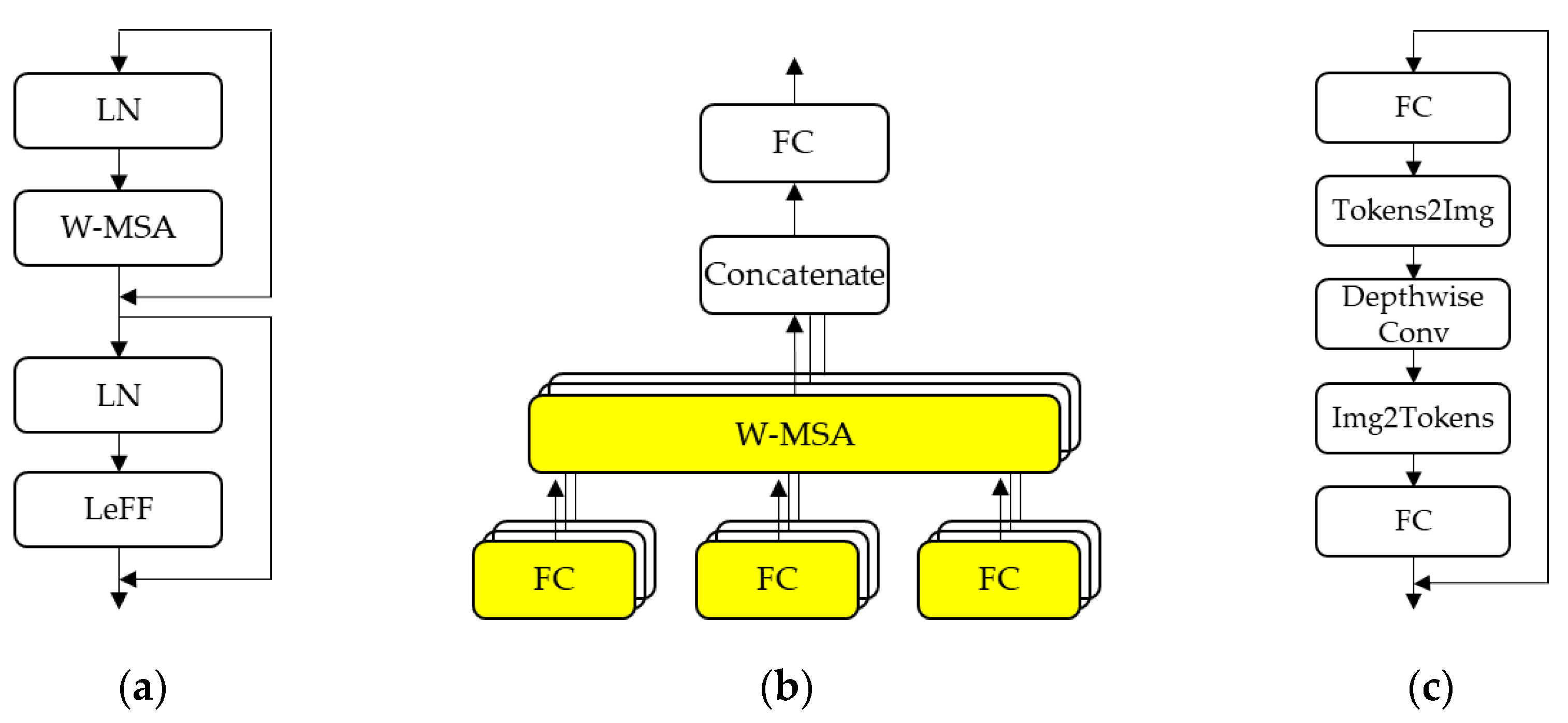
3.2. Image Deblurring Using Transformer

There are many deep learning model architectures for defocus deblurring. A popular approach for image processing is the U-Net architecture [37], which is characterized by its encoder–decoder structure as well as skip connections.
In recent years, Transformer has been quite competitive compared to convolutional neural networks. After evaluating several model architectures, we have chosen the model by Wang [23], which employs U-Net architecture and Transformer block. The model architecture is shown in Figure 5. The model consists of three main modules: input (output) projection, Transformer block and down (up) sampling. The main purpose of the input projection is to convert the data into a format that can be processed by the Transformer block, and the output projection converts the processed data into images. Down sampling is used to compress the size of the feature map and reduce the computational cost, while up sampling is used to restore the compressed feature map to its original size. Skip connections in the model can preserve previously learned features across network layers.
The Transformer block is a key component of the network. It uses a window-based multi-headed self-attention (W-MSA) mechanism to map feature maps to different spaces and improve feature extraction. A locally enhanced feed-forward (LeFF) network is also used in the Transformer block to enhance the ability to capture local contextual information. The structure of the Transformer block is shown in Figure 6. Each Transformer block is composed of LayerNorm (LN) layer, W-MSA block, LeFF block and skip connections. The architecture of how W-MSA block works is shown in Figure 6b. It is able to improve the feature extraction by mapping to different spaces through QKV. All the cropped feature maps are compressed by a full connection (FC) layer and sent to the W-MSA block to calculate the attention value. The structure of the LeFF block is shown in Figure 6c. It is a new structure formed by adding a depthwise convolution to the Feed-Forward Network (FFN) of the standard Transformer block. FFN has limitations in capturing local contextual information and adding depthwise convolution to an FFN can enhance the ability to capture local contextual information.
The loss function used to train the model is
L ( I , I g t ) = I I g t 2 + ε 2
where I′ is the output image, Igt is the ground-truth image, and ε (10−3) is a constant.
To train the model, sharp images are chosen from the DPDD dataset [20] and cropped to non-overlapping images of size 256 × 256 pixels. According to Equation (14), each cropped image is convolved with the system transfer function to generate the blur image. From Section 2.2, we know that MTFsys will be changed when the system parameters change, and PSFwater will be changed when the condition of the water is changed. Thus, to enable the model to deal with different levels of blurred image, 16 different blur kernels are generated according to Equation (14) by changing the parameters of focal length and attenuation coefficient of the water.

4. Results and Discussion

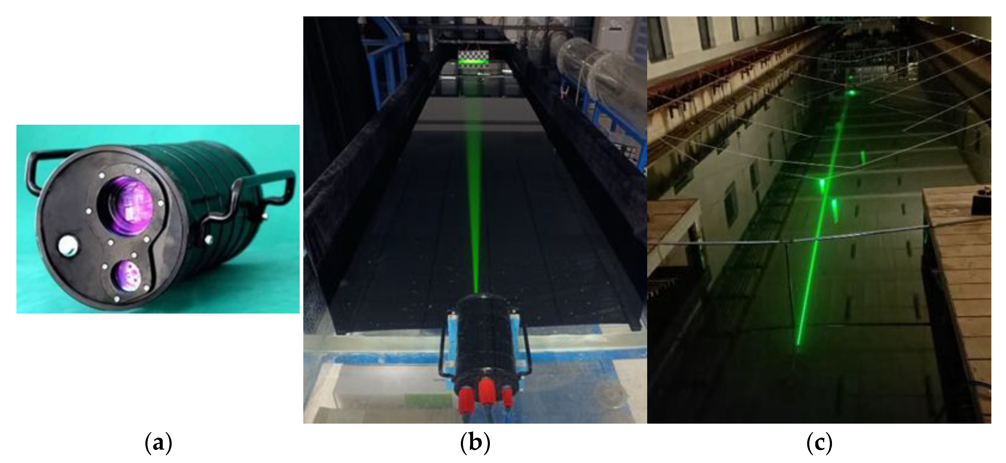
4.1. Experimental Setup

To verify the methods in this paper, two experiments are carried out in a laboratory water tank and a boat tank at Huazhong University of Science and Technology. The imaging system used in the experiments and the experimental scenario are shown in Figure 7.
The PLRGI system used in the experiments is shown in Figure 7a. The laser works at a repetition rate of 10 kHz with a pulse length of 5 ns. The minimum gate width is 5 ns, and the maximum frame rate is 30 Hz. Some characteristics of the system are listed in Table 1, and more information about the system can be acquired from the literature [8].
The water tank is 7 m long, 0.5 m high and 1 m wide. The size of the towing boat tank is 175 m × 6 m × 4 m (length × width × depth). The attenuation coefficient of the water was estimated [38] to 0.15 m−1 and 0.25 m−1, respectively.

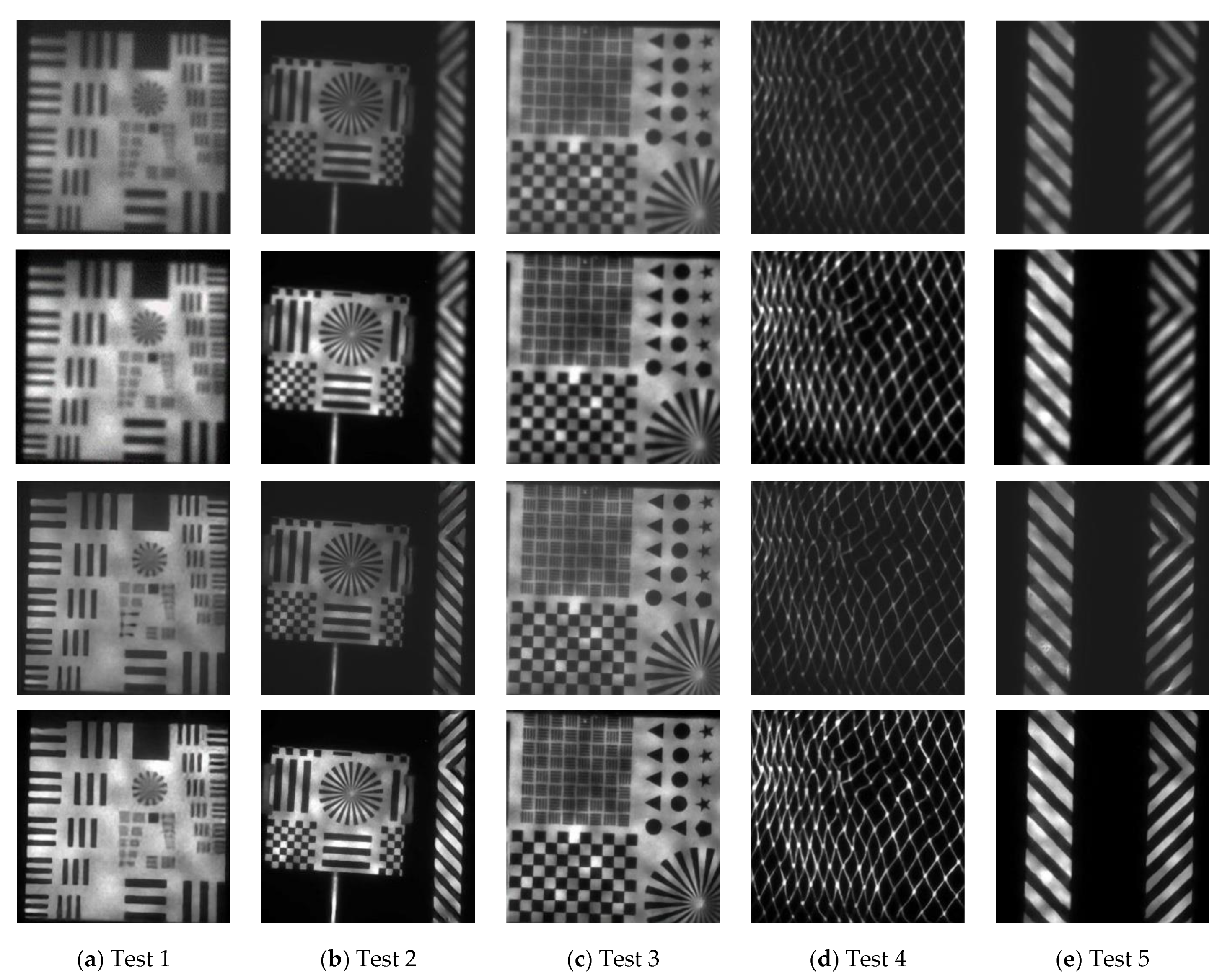
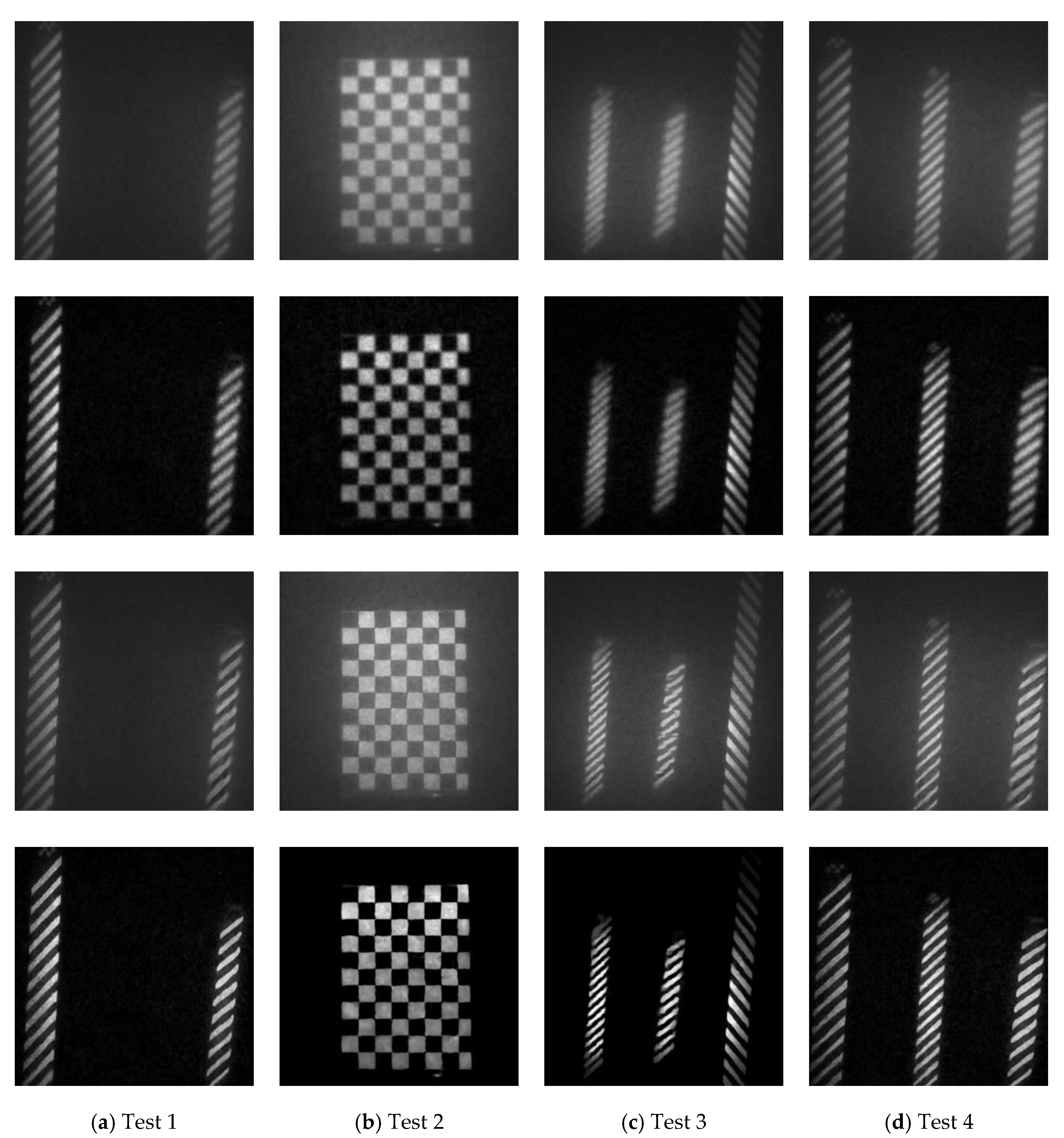
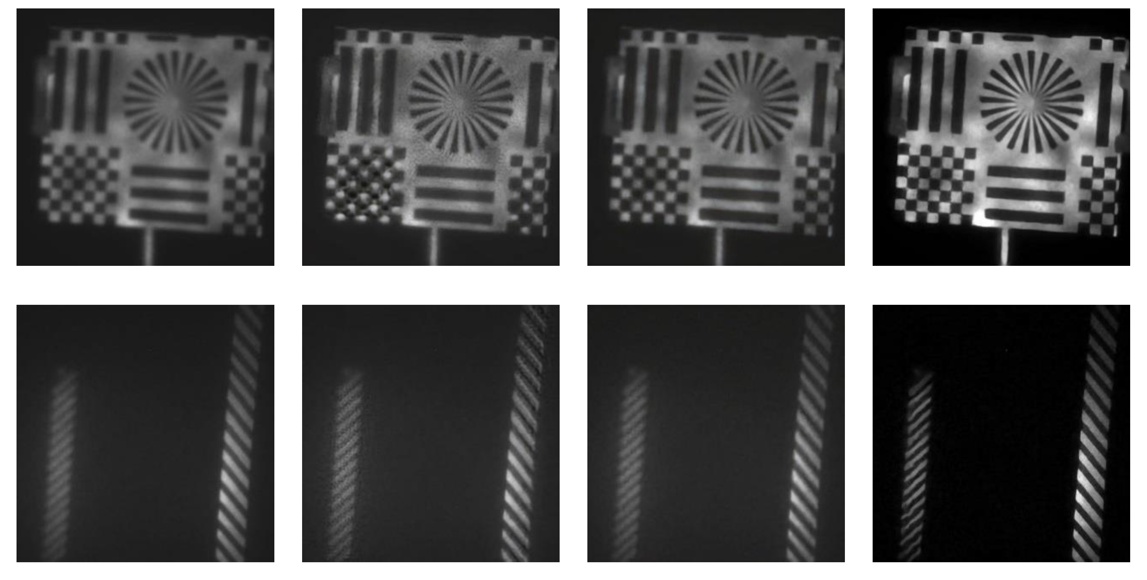
4.2. Experiments in the Water Tank

Many images of varying degrees of blur were collected in a water tank as a test set, five of which are shown in Figure 8.
As can be seen in Figure 8, the contrast of the image is improved after the backscattered light is removed, but the blurring remains. To facilitate the description, the first row (the original data) of Figure 8 is denoted as ORI, the second row (data after the removal of backscattered light) as SUB, the third row (result of the deblurring of the first row) as ORI-deblur, and the fourth row (result of the deblurring of the second row) as SUB-deblur. Images of both ORI-deblur and SUB-deblur are sharper than those of ORI or SUB, and due to the influence of backscattered light, images of ORI-deblur are more blurred than those of SUB-deblur. Compared to ORI, the sharpness of the images of SUB-deblur increases significantly. In addition, we can see that the trained model can deblur images of different degrees of blur.
The Brenner gradient is often used to evaluate the sharpness of an image. It is expressed as,
f ( I )   =   x y [ I ( x + 2 , y ) I ( x , y ) ] 2
where I(x,y) is the gray value.
A comparison of images from Figure 8 by Brenner gradient is shown in Figure 9.
From Figure 9, we can see that the Brenner gradient of images from SUB-deblur are much larger than those from others, and this means that images from SUB-deblur are much sharper than those from others.

4.3. Experiments in the Boat Tank

Many images were collected in a boat tank by the PLRGI system with the MSI method, four of which are shown in Figure 10.
As can be seen in Figure 10, images of the first row were collected by the PLRGI system with large DOV, and some targets are out of focus. In addition, due to the large attenuation coefficient, backscattered light is obvious.
We can see from the second row that most of the backscattered light is removed, and the contrast of the images is improved. Images of both ORI-deblur and SUB-deblur are sharper than that of ORI or SUB, and due to the influence of backscattered light, images of ORI-deblur are not that clear. Compared to ORI, the sharpness of the images of SUB-deblur increases significantly. In addition, the trained model can deblur images of different levels of blur and can deal with images which have sharp targets and blurred targets.
A comparison of images from Figure 10 by Brenner gradient is shown in Figure 11.
From Figure 11, we can see that the Brenner gradient of images from SUB-deblur are much larger than those from others, and this means that images from SUB-deblur are much sharper than those from others. This is consistent with the subjective feelings.

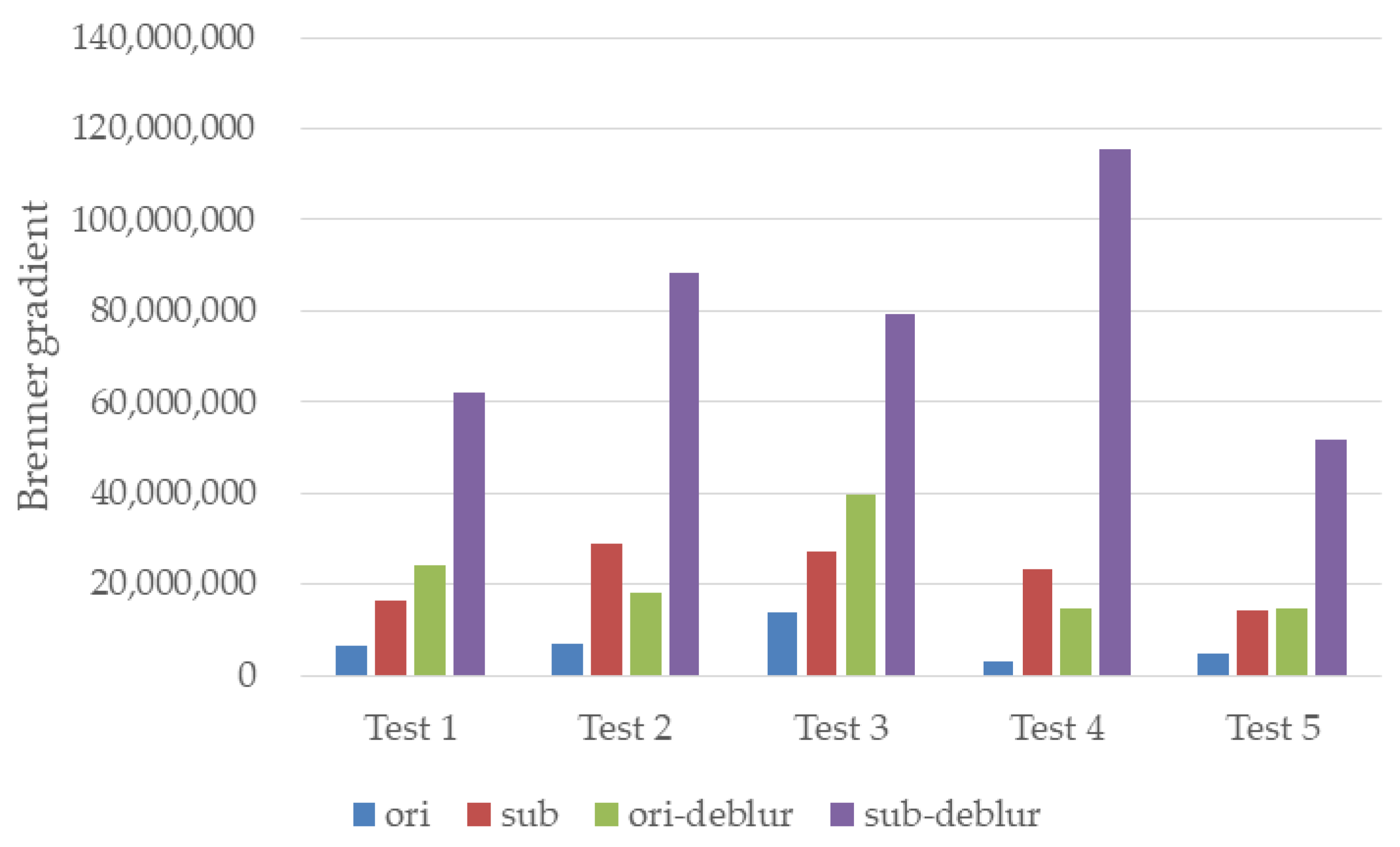
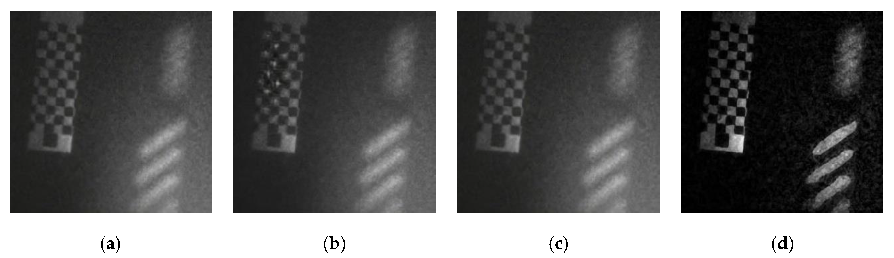
4.4. Compare with Other Methods

We compare our method with the recent end-to-end deep-learning-based approach for defocus deblurring [21,22]. The result images are produced by using the pre-trained model provided by the authors. KPAC provides two versions of models, one is 2-level KPAC and the other is 3-level KPAC. We choose 2-level KPAC to deblur the images. For evaluation, we measure the Brenner gradient of the images.
Figure 12 shows a qualitative comparison. As the figure shows, our method produces sharper results with more details. KPAC is affected by noise severely and has a small effect on large-scale blur. GKMNet has little effect with large-scale blur.
Table 2 reports the quantitative comparison. As shown in the table, our method performs better than KPAC and GKMNet, which is consistent with the subjective feelings.

5. Conclusions

We have introduced an underwater image deblurring method for the PLRGI system with an MSI method. Our method considers the blur caused by the combined effect of forward scattering and defocus. According to the imaging model, we introduce the rolling ball and intensity transformation to remove backscattered light before deblurring, and we introduce a deep learning model based on Transformer to deblur images with different levels of blur. Extensive experiments on various water conditions were carried out, and the results show that the proposed method is effective and robust. The imaging model and the backscattered light removal method in this paper is also beneficial for other underwater vision tasks. Although the deep learning model based on Transformer has good performance in deblurring, it takes too much time and cannot handle this in real time. In order to be applied to the compact system, this issue will be studied in our future work.

Author Contributions

All experiments were carried out and analyzed by all authors. H.L. wrote the manuscript, which was discussed by all authors. All authors have read and agreed to the published version of the manuscript.

Funding

This research was funded by Independent Scientific Research Project of Naval University of Engineering (20200357).

Institutional Review Board Statement

Not applicable.

Informed Consent Statement

Not applicable.

Data Availability Statement

The data that support this study are proprietary in nature and may only be provided with restrictions.

Acknowledgments

The authors thank Huazhong University of Science and Technology for the support of experiment in the boat tank. The authors thank Zhang Su, Kai Li and Sun Chunsheng for the help during the experiment.

Conflicts of Interest

The authors declare no conflict of interest.

References

  1. Liu, X.; Wang, X.; Ren, P.; Cao, Y.; Zhou, Y.; Liu, Y. Automatic Fishing Net Detection and Recognition Based on Optical Gated Viewing for Underwater Obstacle Avoidance. Opt. Eng. 2017, 56, 83101. [Google Scholar] [CrossRef]
  2. Risholm, P.; Thorstensen, J.; Thielemann, J.T.; Kaspersen, K.; Tschudi, J.; Yates, C.; Softley, C.; Abrosimov, I.; Alexander, J.; Haugholt, K.H. Real-Time Super-Resolved 3D in Turbid Water Using a Fast Range-Gated CMOS Camera. Appl. Opt. 2018, 57, 3927–3937. [Google Scholar] [CrossRef] [PubMed]
  3. Sluzek, A. Model of Gated Imaging in Turbid Media. Opt. Eng. 2005, 44, 116002. [Google Scholar] [CrossRef]
  4. Ulich, B.L.; Lacovara, P.; Moran, S.E.; DeWeert, M.J. Recent Results in Imaging Lidar. In Proceedings of the Advances in Laser Remote Sensing for Terrestrial and Oceanographic Applications, Orlando, FL, USA, 21–22 April 1997; SPIE: Bellingham, WA, USA, 1997; Volume 3059, pp. 95–108. [Google Scholar]
  5. McLean, E.A.; Burris, H.R.; Strand, M.P. Short-Pulse Range-Gated Optical Imaging in Turbid Water. Appl. Opt. 1995, 34, 4343–4351. [Google Scholar] [CrossRef] [PubMed]
  6. Acharekar, M.A. Underwater Laser Imaging System (ULIS); Dubey, A.C., Barnard, R.L., Eds.; SPIE: Orlando, FL, USA, 1997; Volume 3079, pp. 750–761. [Google Scholar]
  7. Xinwei, W.; Youfu, L.; Yan, Z. Multi-Pulse Time Delay Integration Method for Flexible 3D Super-Resolution Range-Gated Imaging. Opt. Express 2015, 23, 7820–7831. [Google Scholar] [CrossRef]
  8. Lin, H.; Han, H.; Ma, L.; Ding, Z.; Jin, D.; Zhang, X. Range Intensity Profiles of Multi-Slice Integration for Pulsed Laser Range-Gated Imaging System. Photonics 2022, 9, 505. [Google Scholar] [CrossRef]
  9. Chen, Y. Model-Based Restoration and Reconstruction for Underwater Range-Gated Imaging. Opt. Eng. 2011, 50, 113203. [Google Scholar] [CrossRef]
  10. Murez, Z.; Treibitz, T.; Ramamoorthi, R.; Kriegman, D.J. Photometric Stereo in a Scattering Medium. IEEE Trans. Pattern. Anal. Mach. Intell. 2017, 39, 1880–1891. [Google Scholar] [CrossRef]
  11. Fujimura, Y.; Iiyama, M.; Hashimoto, A.; Minoh, M. Photometric Stereo in Participating Media Using an Analytical Solution for Shape-Dependent Forward Scatter. IEEE Trans. Pattern Anal. Mach. Intell. 2020, 42, 708–719. [Google Scholar] [CrossRef] [PubMed]
  12. Drews, P.L.J.; Nascimento, E.R.; Botelho, S.S.C.; Montenegro Campos, M.F. Underwater Depth Estimation and Image Restoration Based on Single Images. IEEE Comput. Graph. Appl. 2016, 36, 24–35. [Google Scholar] [CrossRef]
  13. Li, C.; Anwar, S.; Hou, J.; Cong, R.; Guo, C.; Ren, W. Underwater Image Enhancement via Medium Transmission-Guided Multi-Color Space Embedding. IEEE Trans. Image Process. 2021, 30, 4985–5000. [Google Scholar] [CrossRef]
  14. Zhang, W.; Zhuang, P.; Sun, H.-H.; Li, G.; Kwong, S.; Li, C. Underwater Image Enhancement via Minimal Color Loss and Locally Adaptive Contrast Enhancement. IEEE Trans. Image Process. 2022, 31, 3997–4010. [Google Scholar] [CrossRef]
  15. Zhang, W.; Dong, L.; Xu, W. Retinex-Inspired Color Correction and Detail Preserved Fusion for Underwater Image Enhancement. Comput. Electron. Agric. 2022, 192, 106585. [Google Scholar] [CrossRef]
  16. Wang, R.; Wang, G. Single Image Recovery in Scattering Medium by Propagating Deconvolution. Opt. Express 2014, 22, 8114. [Google Scholar] [CrossRef]
  17. Risholm, P.; Thielemann, J.T.; Moore, R.; Haugholt, K.H. A Scatter Removal Technique to Enhance Underwater Range-Gated 3D and Intensity Images. In Proceedings of the OCEANS 2018 MTS/IEEE, Charleston, SC, USA, 22–25 October 2018; pp. 1–6. [Google Scholar]
  18. Cun, X.; Pun, C.-M. Defocus Blur Detection via Depth Distillation. In Computer Vision–ECCV 2020; Vedaldi, A., Bischof, H., Brox, T., Frahm, J.-M., Eds.; Lecture Notes in Computer Science; Springer International Publishing: Berlin/Heidelberg, Germany, 2020; Volume 12358, pp. 747–763. ISBN 978-3-030-58600-3. [Google Scholar]
  19. Karaali, A.; Jung, C.R. Edge-Based Defocus Blur Estimation With Adaptive Scale Selection. IEEE Trans. Image Process. 2018, 27, 1126–1137. [Google Scholar] [CrossRef]
  20. Abuolaim, A.; Brown, M.S. Defocus Deblurring Using Dual-Pixel Data. In Proceedings of the Computer Vision–ECCV 2020; Vedaldi, A., Bischof, H., Brox, T., Frahm, J.-M., Eds.; Springer International Publishing: Berlin/Heidelberg, Germany, 2020; Volume 12355, pp. 111–126. [Google Scholar]
  21. Son, H.; Lee, J.; Cho, S.; Lee, S. Single Image Defocus Deblurring Using Kernel-Sharing Parallel Atrous Convolutions. In Proceedings of the 2021 IEEE/CVF International Conference on Computer Vision (ICCV); IEEE: Montreal, QC, Canada, 2021; pp. 2622–2630. [Google Scholar]
  22. Quan, Y.; Wu, Z.; Ji, H. Gaussian Kernel Mixture Network for Single Image Defocus Deblurring. arXiv 2021, arXiv:2111.00454. [Google Scholar]
  23. Wang, Z.; Cun, X.; Bao, J.; Zhou, W.; Liu, J.; Li, H. Uformer: A General U-Shaped Transformer for Image Restoration. arXiv 2021, arXiv:2106.03106. [Google Scholar]
  24. Zamir, S.W.; Arora, A.; Khan, S.; Hayat, M.; Khan, F.S.; Yang, M.-H. Restormer: Efficient Transformer for High-Resolution Image Restoration. arXiv 2022, arXiv:2111.09881. [Google Scholar]
  25. Jaffe, J.S. Computer Modeling and the Design of Optimal Underwater Imaging Systems. IEEE J. Ocean. Eng. 1990, 15, 101–111. [Google Scholar] [CrossRef]
  26. McGlamery, B.L. A Computer Model for Underwater Camera Systems; Duntley, S.Q., Ed.; SPIE: Monterey, CA, USA, 1979; Volume 0208, pp. 221–231. [Google Scholar]
  27. Hou, W.; Gray, D.J.; Weidemann, A.D.; Arnone, R.A. Comparison and Validation of Point Spread Models for Imaging in Natural Waters. Opt. Express 2008, 16, 9958. [Google Scholar] [CrossRef]
  28. Zhang, W.; Liu, H.; Zou, P.; Chen, Q.; Gu, G.; Zhang, L. Research on Modulation Transfer Function of the Electron Multiplying CCD. In Proceedings of the 2012 Symposium on Photonics and Optoelectronics, Shanghai, China, 21–23 May 2012; IEEE: Shanghai, China, 2012; pp. 1–4. [Google Scholar]
  29. Wu, L.; Shen, Y.; Li, G.; Chen, C.; Yang, H. Modeling and Simulation of Range-Gated Underwater Laser Imaging Systems; Amzajerdian, F., Gao, C., Xie, T., Eds.; SPIE: Beijing, China, 2009; Volume 7382, p. 73825B. [Google Scholar]
  30. Holst, G.C. CCD Arrays, Cameras, and Displays, 2nd ed.; SPIE Optical Engineering: Winter Park, CO, USA; JCD Publishing: Bellingham, FL, USA, 1998; ISBN 978-0-9640000-4-9. [Google Scholar]
  31. Csorba, I.P. Modulation Transfer Function (MTF) Of Image Intensifier Tubes; Williams, T.L., Ed.; SPIE: Reading, UK, 1981; Volume 0274, pp. 42–51. [Google Scholar]
  32. Sun, L.; Wang, X.; Liu, X.; Ren, P.; Lei, P.; He, J.; Fan, S.; Zhou, Y.; Liu, Y. Lower-Upper-Threshold Correlation for Underwater Range-Gated Imaging Self-Adaptive Enhancement. Appl. Opt. 2016, 55, 8248. [Google Scholar] [CrossRef]
  33. Kaiming He; Jian Sun; Xiaoou Tang Single Image Haze Removal Using Dark Channel Prior. IEEE Trans. Pattern Anal. Mach. Intell. 2011, 33, 2341–2353. [CrossRef]
  34. Rodrigues, M.; Militzer, M. Application of the Rolling Ball Algorithm to Measure Phase Volume Fraction from Backscattered Electron Images. Mater. Charact. 2020, 163, 110273. [Google Scholar] [CrossRef]
  35. Rashed, M. Rolling Ball Algorithm as a Multitask Filter for Terrain Conductivity Measurements. J. Appl. Geophys. 2016, 132, 17–24. [Google Scholar] [CrossRef]
  36. Sternberg Biomedical Image Processing. Computer 1983, 16, 22–34. [CrossRef]
  37. Ronneberger, O.; Fischer, P.; Brox, T. U-Net: Convolutional Networks for Biomedical Image Segmentation. In Medical Image Computing and Computer-Assisted Intervention–MICCAI 2015; Navab, N., Hornegger, J., Wells, W.M., Frangi, A.F., Eds.; Lecture Notes in Computer Science; Springer International Publishing: Cham, Switzerland, 2015; Volume 9351, pp. 234–241. ISBN 978-3-319-24573-7. [Google Scholar]
  38. Lin, H.; Zhang, X.; Ma, L.; Hu, Q.; Jin, D. Estimation of Water Attenuation Coefficient Byimaging Modeling of the Backscattered Lightwith the Pulsed Laser Range-Gated Imagingsystem. Opt. Contin. 2022, 1, 989–1002. [Google Scholar] [CrossRef]
Figure 1. Description and time sequence of the MSI method with three slices: (a) three targets are in three adjacent slices respectively; (b) time sequence of the MSI method. The same delay time belongs to the same slice, the gate width is small, and only one target echo can be passed.
Photonics 09 00642 g001
Figure 2. Composition of the receiver in the PLRGI system.
Photonics 09 00642 g002
Figure 3. Flowchart of the proposed method.
Photonics 09 00642 g003
Figure 4. Description of rolling ball background subtraction algorithm: (a) underwater image captured by PLRGI system; (b) calculated background of line A-B by rolling ball; (c) corrected profile.
Photonics 09 00642 g004
Figure 5. Model architectures for image deblurring.
Photonics 09 00642 g005
Figure 6. Description of the Transformer block: (a) Transformer block; (b) illustration of how the W-MSA works; (c) structure of LeFF.
Photonics 09 00642 g006
Figure 7. The PLRGI system and experimental scenario: (a) the PLRGI system used in the experiments; (b) water tank in lab; (c) boat tank.
Photonics 09 00642 g007
Figure 8. Image deblurring result of the test set. The first row is the original data (denoted by ORI), the second row is the data with the removal of backscattered light (denoted by SUB), the third row is the result of the deblurring of the first row images (denoted by ORI-deblur), and the fourth row is the blur removal result for the second row images (denoted by SUB-deblur).
Photonics 09 00642 g008
Figure 9. Comparison of images from Figure 8 by the Brenner gradient.
Photonics 09 00642 g009
Figure 10. Image deblurring results. The first row is the original data (denoted by ORI), the second row is the data with the removal of backscattered light (denoted by SUB), the third row is the result of the deblurring of the first row images (denoted by ORI-deblur), and the fourth row is the blur removal result for the second row images (denoted by SUB-deblur).
Photonics 09 00642 g010
Figure 11. Comparison of images from Figure 10 by the Brenner gradient.
Photonics 09 00642 g011
Figure 12. Visual comparison of three methods. The first row, the second row and the third row denoted as Test 1, Test 2 and Test 3: (a) images captured by PLRGI system; (b) results of KPAC (2-level); (c) results of GKMNet; (d) results of our proposed method.
Photonics 09 00642 g012aPhotonics 09 00642 g012b
Table 1. Characteristics of the PLRGI system.
SpecificationsCharacteristics
DimensionsΦ150 mm × L280 mm
Weight in water≤1 kg
Depth rangeUp to 200 m
Camera Lens8–48 mm focal length
Field Of View50°
Frame rate1–30 Hz
Visual rangeUp to 5 attenuation lengths
Table 2. Brenner gradient of the images in Figure 12.
ImageOriginal-ImgKPAC (2-Level)GKMNetProposed
Test 16,332,71711,105,33216,595,90160,484,160
Test 21,859,7692,309,7264,788,04412,987,654
Test 31,711,6703,133,3174,259,16722,433,318
Publisher’s Note: MDPI stays neutral with regard to jurisdictional claims in published maps and institutional affiliations.

