Speckle Noise Suppression Based on Empirical Mode Decomposition and Improved Anisotropic Diffusion Equation

Abstract

Existing methods to eliminate the laser speckle noise in quantitative phase imaging always suffer from the loss of detailed phase information and the resolution reduction in the reproduced image. To overcome these problems, this paper proposes a speckle noise suppression method based on empirical mode decomposition. Our proposed method requires only one image without additional equipment and avoids the complicated process of searching the optimal processing parameters. In this method, we use empirical mode decomposition to highlight the high frequency information of the interference image and use the Canny operator to perform edge detection, so the diffusion denoising process is guided by high-precision detection results to achieve better results. To validate the performance of our proposed method, the phase maps processed by our proposed method are compared with the phase maps processed by the improved anisotropic diffusion equation method with edge detection, the mean filter method and the median filter method. The experimental results show that the method proposed in this paper not only has a better denoising effect but also preserves more details and achieves higher phase reconstruction accuracy.

1. Introduction

Quantitative phase imaging [1,2,3,4] (QPI) is an emerging label-free optical imaging method that enables visualization of the three-dimensional topography of reflective samples or measurement of the internal structure or refractive index distribution of transparent and translucent samples. Its application on transparent biological samples is one of the existing research trends in bio-optical imaging. It mainly relies on holography and interference technology to record the phase distribution of the transparent object or extracts the phase of the object from the diffraction intensity map of the recorded light field passing through the transparent object. It can be combined with compressive sensing [5,6,7], deep learning [8,9,10], autofocus [11,12,13], topological modulation [14,15] or compensation techniques [16,17,18] to achieve higher precision measurement results.

At present, a laser is often used as a light source for QPI. Due to the high coherence of the laser and the high roughness of the object, the scattered light is coherently superimposed on the interference plane to form speckle noise [19]. Speckle reduces the contrast and resolution of the reconstructed image [20], limiting the application of QPI. Therefore, it is necessary to suppress the laser speckle noise.

The commonly used methods for speckle noise suppression are mainly divided into two categories. One is to add or replace hardware to reduce the coherence of the light source, such as using low-coherence LED light sources [21]. Choi et al. [22] developed an off-axis quantitative phase microscopy system that relies on light sources with extremely short spatial coherence lengths. The system is able to reduce diffraction noise while improving spatial resolution. Farrokhi et al. [23] adopted a dynamic and static dual diffuser system to obtain high-speed speckle field illumination to suppress coherent speckle in QPI. This type of hardware method generally requires higher precision control of the optical path difference in the optical path, which increases the complexity and difficulty of constructing the optical path. Another category is achieving speckle noise suppression through image processing. The mean filter method [24] and the median filter method [25] are the kernel-based noise reduction methods in digital image processing which can blur image details and reduce the accuracy of phase map reconstruction. Uzan et al. [26] applied a non-local mean (NLM) filtering algorithm to pixels located in the center of the image block, which had a good suppression effect on speckle noise. However, this method smooths the information at some edges while denoising, which leads to phase errors. Montresor et al. [27] applied a residual network (DNCNN) to denoise the phase map of digital holographic interferometry, which has non-Gaussian statistics and non-stationary properties and exhibits spatial correlation length with excellent denoising performance. This method needs to use a large number of hologram datasets with speckle noise to train multi-level neural networks, and the experimental conditions are complicated. Niu et al. [28] proposed using a two-dimensional Gaussian window to suppress the speckle noise of the wrapped phase, which improves the accuracy of phase reconstruction. In this method, the size of the two-dimensional Gaussian window and the threshold affects the phase reconstruction accuracy, and thus it is necessary to study the optimal window size and threshold. Gao et al. [29] established an anisotropic diffusion model to suppress speckle noise based on anisotropic diffusion in additive noise, which can effectively remove the speckle noise and retain minute details of the image. However, this method should establish an anisotropic diffusion model in advance, and the optimal values of its parameters should be obtained through learning, which is a complicated and time-consuming computational process. Wu et al. [30] proposed a holographic speckle suppression method based on the Canny operator to improve the anisotropic diffusion equation. This method has a slight improvement in retaining the detailed information of the image, but the accuracy of the recovered phase map should be further improved.

To overcome these problems, this paper proposes a QPI speckle noise suppression method, which combines the Canny operator of empirical mode decomposition (EMD) to improve the anisotropic (P-M) diffusion equation. Only one phase imaging result is required in our proposed method. The method proposed in this paper first performs EMD on the recorded interferogram and reconstructs the image using only the decomposed high-frequency intrinsic mode function (IMF) components to enhance the detailed information of the image. Then, the Canny operator is introduced to perform edge detection, which has a better control on the diffusion denoising process and improves the performance of the P-M diffusion equation (P-M equation for short) to suppress speckle noise. The feasibility of the speckle noise suppression method has been verified by experiments.

The remaining sections of this paper are organized as follows. Section 2 presents the proposed method of this paper in detail. Section 3 shows the experimental results and result analysis. Section 4 presents the discussion on the proposed methods. Section 5 concludes the whole paper.

2. Principles

Speckle noise in the interferogram is a uniformly distributed noise [31] whose mathematical model is as follows:

$$H^{\prime }(x,y)=H(x,y)N(x,y)$$

(1)

where $H^{\prime }(x,y)$ is an interferogram recorded by a charge coupled device (CCD), which contains speckle noise; $H(x,y)$ is an ideal interferogram without noise; and $N(x,y)$ is speckle noise. Our method aims to eliminate the speckle noise $N(x,y)$ from the recorded interferogram $H^{\prime }(x,y)$.

To suppress speckle noise, the method proposed in this paper first performs EMD on the recorded interferogram to obtain a series of IMF components from high to low frequencies, and only the high-frequency IMF components are used to reconstruct the image to enhance the image detail information. Then the Canny operator is introduced to detect the edge of the reconstructed image with prominent detail information, which guides the P-M equation to achieve a better denoising effect.

2.1. Empirical Mode Decomposition (EMD)

We decompose the two-dimensional signal $f(x,y)$ into a series of IMF components with frequencies ranging from high to low. The high-frequency part contains object detail information and the low-frequency part contains object outline information. Images with different characteristics can be obtained by selecting IMFs with different frequencies to reconstruct images. For example, if the image should be degraded to reduce the influence of noise, only the low-frequency IMF components are selected to reconstruct a new image; if the image details should be highlighted to enhance the image, only the high-frequency IMF components are selected to reconstruct a new image. The process of EMD is as follows:

1.

Find the maxima and minima of $f(x,y)$ and construct the maximum surface $u(x,y)$ and the minimum surface $v(x,y)$ by interpolation. Then, the mean of the maximum surface and the minimum surface is:

$$e_1(x,y)=\frac{u(x,y)+v(x,y)}{2}$$

(2)

and the difference between the mean $e_1(x,y)$ and $f(x,y)$ is recorded as $h_1(x,y)$,

$$h_1(x,y)=f(x,y)-e_1(x,y)$$

(3)

2.

Repeat the above process $k$ times until the Formula (4) is satisfied. Among them, the value of $SD$ generally falls within 0.1–0.5 and $\alpha$ is generally 0.2.

$$SD={\displaystyle \sum _{x=1}^X{\displaystyle \sum _{y=1}^Y\frac{{\left|h_{1(k-1)}(x,y)-h_{1k}(x,y)\right|}^2}{h_{1k}{}^2(x,y)}}}\le \alpha$$

(4)

It is worth noting that the expression of $SD$ is actually the standard deviation calculation formula between the calculation results of two adjacent iterations. When $SD\le \alpha$, it means that the difference between the calculation results $h_{1(k-1)}(x,y)$ and $h_{1k}(x,y)$ is very small, and thus the calculation accuracy has been reached. At this time, the calculated $h_{1k}(x,y)$ is an IMF component, denoted as $C_1$, which contains the highest frequency information of the image.

3.

Let $r_1(x,y)$ denote the remaining part of $f(x,y)$ after removing the highest frequency information $C_1$,

$$r_1(x,y)=f(x,y)-C_1$$

(5)

4.

Let $r_1(x,y)$ be the new image to be analyzed; after repeating the calculation process of steps 1 and 2, the second IMF component $C_2$ is obtained.

5.

Repeat the above process $n$ times, when $r_n(x,y)$ and $C_n$ are smaller than the predetermined error or $r_n(x,y)$ is a monotonic function, the IMF component can no longer be extracted from $f(x,y)$. At this time, $f(x,y)$ can be represented as follows:

$$f(x,y)={\displaystyle \sum _{i=1}^n{C}_i}+r$$

(6)

2.2. The Improved P-M Equation Method with Canny Operator

Image denoising methods based on partial differential equations have been widely used and eventually developed from linear uniform diffusion to anisotropic diffusion. In anisotropic diffusion, the Perona–Malik (P-M) equation is the most widely used [32], and many methods were developed based on the P-M diffusion equation [33,34,35].

The traditional P-M equation has the following problems:

• Since the gradient operator $\nabla$ cannot remove large isolated noise points, the gradient value at large noise points will be large. At the same time, the diffusion coefficient $c$ is inversely proportional to the gradient value, which will cause the value of the diffusion coefficient $c$ here to become smaller and the effect of diffusion denoising cannot be achieved.
• Gradient operator $\nabla$ is highly sensitive to noise, and its anti-noise performance is not strong; thus, it cannot identify the false edges.

In order to overcome the above problems, the P-M equation is improved by introducing the Canny edge detection operator to overcome the problem that the gradient operator $\nabla$ is not strong in anti-noise. At this time, the P-M equation can be rewritten as

$$\frac{\partial I(x,y,t)}{\partial t}=div[(1-K)\cdot c(\left|\nabla I(x,y,t\right|))\cdot \nabla I(x,y,t)]$$

(7)

where $t$ is the time, $I(x,y,0)$ is the initial state, $K$ is the Canny operator, $\nabla$ is the gradient operator, $div$ is the divergence operator. $c$ is the diffusion coefficient, which is used to control the degree of diffusion of the P-M equation. There are two commonly used calculation formulas, as shown below.

$$c(x)=\exp (-{\left(x/k\right)}^2)$$

(8)

$$c(x)=\frac{1}{1+{(x/k)}^2}$$

(9)

In Equations (8) and (9), $k$ is a coefficient that controls the diffusion process. The two formulas are almost equivalent when $x/k$ is relatively small.

Perform Canny edge detection on the image $g(x,y)$ to obtain the edge detection result $G(x,y)$ and record the upper threshold $k_1$. When the pixel is the edge of the image, $K$ tends to be 1, which makes the diffusion speed of the P-M equation slow down and preserve the image details. Otherwise, when $K$ tends to be 0, which makes the diffusion speed of the P-M equation accelerated and results in better denoising. Using the Canny operator $K$ to improve the P-M equation has certain advantages. On the one hand, the Canny operator $K$ is less sensitive to noise than the gradient operator $\nabla$ and has better anti-noise ability. On the other hand, the double-threshold screening in Canny edge detection generally covers 70% of the non-edge pixels of the image. It is obviously a reasonable choice to make the parameter $k$ in the diffusion coefficient $c$ equal to the upper threshold $k_1$. After the image is processed by the improved P-M equation method with the Canny operator, it can be expressed as:

$$g\prime (x,y)=g(x,y)+(1-K)div$$

(10)

2.3. The Method Proposed in This Paper

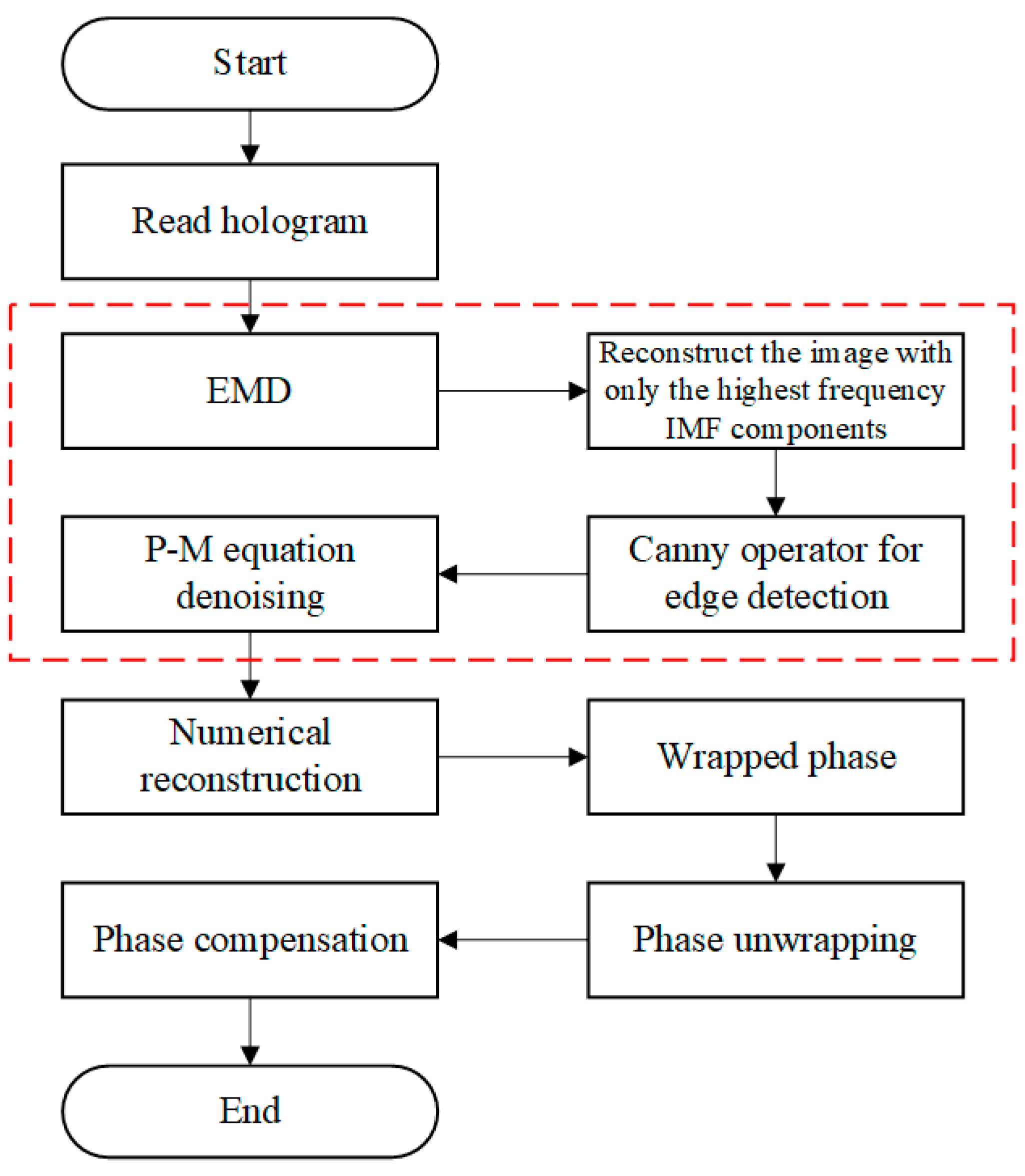
We summarize our proposed speckle noise suppression method as follows:

• Perform EMD decomposition on the image $H^{\prime }(x,y)$; Formula (1) can be rewritten as:

  $$H^{\prime }(x,y)=({\displaystyle \sum _{i=1}^n{C}_i+r})N(x,y)$$

  (11)

Since the detailed information of the interferogram is mainly included in the high-frequency component $C_1$, only the high-frequency component $C_1$ is used to reconstruct the new interferogram. Equation (11) can be rewritten as:

$$H^{″}(x,y)=C_{1}N(x,y)$$

(12)

2.

Perform Canny edge detection on the reconstructed image $H^{″}(x,y)$ to obtain the edge detection result $G(x,y)$ and record the upper threshold $k_1$.

3.

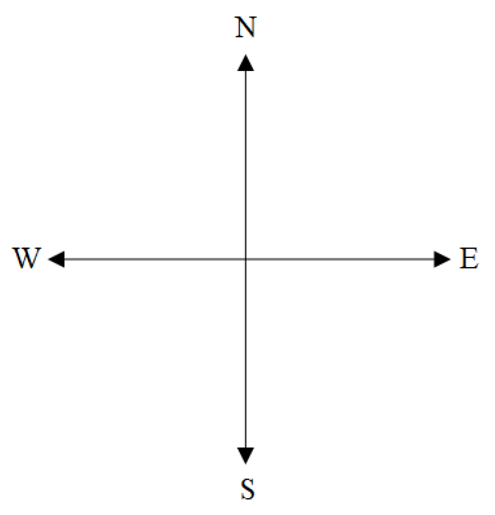
According to the four directions shown in Figure 1, the gradients of the four directions of the image $H^{″}(x,y)$ are solved, namely ${\nabla }_N$, ${\nabla }_S$, ${\nabla }_E$ and ${\nabla }_W$.

4.

Let the parameter $k$ in the diffusion coefficient $c$ be equal to the upper threshold $k_1$, and combine the gradients in the four directions to obtain $c_N$, $c_S$, $c_W$ and $c_E$.

5.

Since there are only two values of 0 and 1 in the Canny edge detection result $G(x,y)$, when $G(x,y)$ is 1, let the Canny operator $K$ be 0.01; when $G(x,y)$ is 0, let the Canny operator $K$ be 0.99.

6.

The divergence operator $div$ can be calculated according to the following formula:

$$div=\frac{1}{4}(c_N\times {\nabla }_N+c_S\times {\nabla }_S+c_E\times {\nabla }_E+c_W\times {\nabla }_W)$$

(13)

After the image $H^{\prime }(x,y)$ is processed by combining the Canny operator of EMD to improve the P-M equation method, it can be expressed as:

$$H^{‴}(x,y)=H^{″}(x,y)+(1-K)div$$

(14)

Then, the interferogram after speckle suppression is numerically reconstructed and the phase information is extracted from the reconstructed image for QPI. Since the phase information is wrapped in $(-\pi ,\pi )$, the phase unwrapping algorithm is performed to obtain the real phase information. Finally, according to the source of the phase error, the corresponding phase compensation algorithm is used to compensate the error. The flowchart of the proposed method in this paper is shown in Figure 2.

3. Experiments and Results Analysis

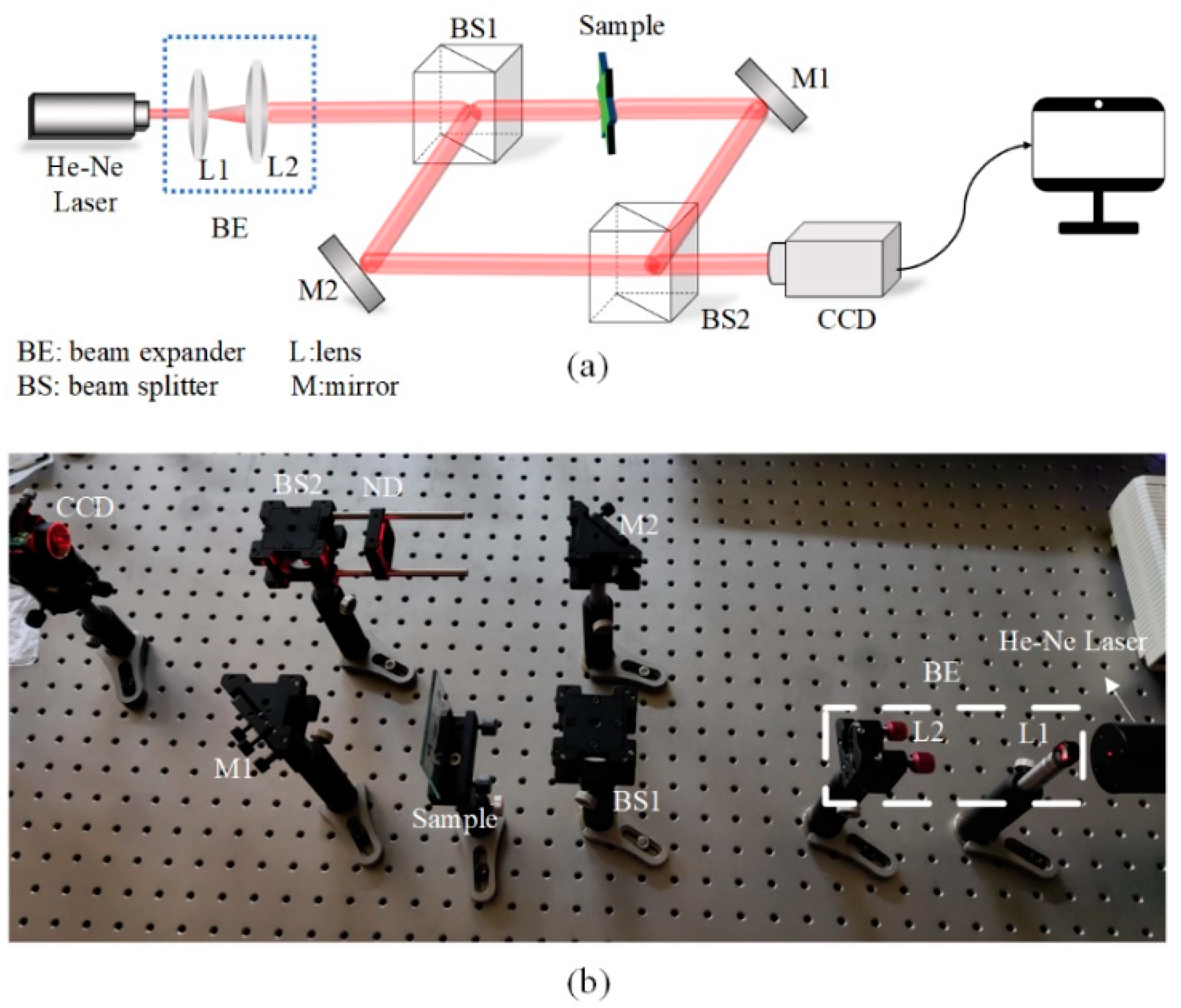
3.1. Experimental Setup

The experimental setup in our study is shown in Figure 3. A He-Ne laser with a wavelength of 632.8 nm is used as the light source. The light emitted by it first passes through a beam expander collimator composed of a plano-concave lens with a focal length of 15 mm and a plano-convex lens with a focal length of 250 mm. It is then split into two beams of equal intensity by split beam BS1. After passing through the sample, a beam is reflected by the mirror M1 to the beam splitter BS2, which is called object light. The other beam is directly reflected by the mirror M2 to BS2, which is called the reference beam. Finally, the object light and the reference light are combined into a beam at BS2 to form an interferogram on the recording surface of the CCD, which is recorded by the CCD.

In the experiment, we use a sample plate shown in Figure 4a and a honeybee foot shown in Figure 4c as samples. Figure 4b,d shows the interferograms of Figure 4a,c recorded by the system shown in Figure 3.

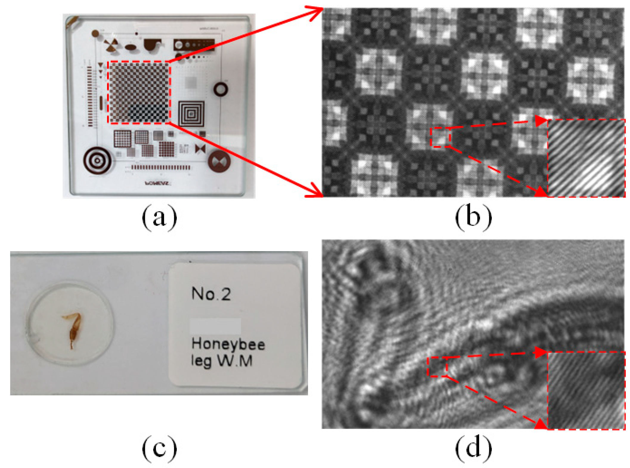
3.2. Quantitative Phase Imaging (QPI)

We perform QPI of Figure 4b,d. Firstly, the interferogram is subjected to EMD to obtain a series of IMF components from high frequency to low frequency, and the images with different effects can be reconstructed by selecting different IMF components. Figure 5 shows the reconstruction of different IMF components of the arbitrarily selected interferogram. Figure 5a–d depicts the reconstructed $C_1$, $C_3$, $C_5$, $C_7$ of Figure 4b, while Figure 5e–h depicts the reconstructed $C_1$, $C_3$, $C_4$, $C_6$ of Figure 4d. It can be clearly observed in the figure that clear stripes can be seen in the image reconstructed by $C_1$, and the reconstructed image becomes increasingly blurred as the frequency of the selected IMF component becomes lower and lower. Therefore, we select the highest frequency IMF component of the interferogram, namely $C_1$, for image reconstruction to highlight the details of the image.

Secondly, Canny operator is used to perform edge detection on the interferogram. Figure 6a,b shows the results of edge detection on Figure 5a and Figure 4b, respectively. Figure 6c,d shows the results of edge detection on Figure 5e and Figure 4d, respectively. By comparison, it can be seen that the edge detection results of (a) and (c) are better.

Thirdly, we use the Canny edge detection results to guide the P-M equation to denoise the interferogram reconstructed from the high-frequency IMF components. Then the angular spectrum diffraction method [36,37,38] is used for numerical reconstruction and the wrapped phase information is recovered from the reconstructed image. The wrapped phase is unwrapped using the discrete cosine-based least squares method [39] to obtain the true phase. Finally, for the digital recording optical path based on the Mach–Zender interferometer, the main source of the phase error is the tilt error introduced between the object light and the reference light. The least-squares fitting method [40] is used for phase compensation. The resulting phase maps is shown in Figure 7 and Figure 8. At the same time, in order to verify the effectiveness of the method proposed in this paper, the proposed method is compared with the improved P-M equation method with Canny operator, the mean filter method and the median filter method.

It can be seen from Figure 7 and Figure 8 that after the speckle noise of interferogram is eliminated, the reconstructed phase maps present a better phase distribution. The distribution of the reconstructed phase maps of the interferogram without denoising is chaotic and irregular. Compared with the other three denoising methods, the reconstructed phase maps after processing by the proposed method in this paper have a smoother contour distribution while retaining the details. For example, after the mean filter method and the median filter method, the bumps of the small squares in Figure 7 are messy and there are obvious missing in the lower left corner of some small squares, and there are two small “hollows” missing in the middle section of Figure 8. The reconstruction results of the improved P-M equation method with the Canny operator are similar to the results of this paper. However, the phase distribution in some regions is not as smooth and full as the reconstructed phase of the method proposed in this paper.

3.3. Quantitative Analysis of Denoising

In order to quantitatively analyze the reconstructed phase map after denoising, this paper adopts structural similarity (SSIM) [41], edge preserving index (EPI) [42] and speckle suppression index (SSI) [43] as indicators for quantitative analysis.

The calculation formula of SSIM is as follows:

$$\mathrm{SSIM}=l(x,y)\cdot c(x,y)\cdot s(x,y)$$

(15)

where $l(x,y)$ represents the brightness of the image, $c(x,y)$ represents the contrast of the image and $s(x,y)$ represents the structure of the image. Generally, the larger the value of SSIM, the smaller the degree of image distortion. When the two images are identical, the value of SSIM is equal to 1.

The formula for calculating EPI is as follows:

$$\mathrm{EPI}=\frac{{\displaystyle \sum _{i=1}^m{\displaystyle \sum _{j=1}^n{\left|G_{R_{11}}-G_{R_{21}}\right|}_{after}}}}{{\displaystyle \sum _{i=1}^m{\displaystyle \sum _{j=1}^n{\left|G_{R_{12}}-G_{R_{22}}\right|}_{before}}}}$$

(16)

where $G_{R_{11}}$ and $G_{R_{21}}$ represent the two adjacent pixels after the image is suppressed and $G_{R_{12}}$ and $G_{R_{22}}$ represent the two adjacent pixels before the image is suppressed. The EPI has a maximum value of 1 and a minimum value of 0. The larger the value of EPI, the better the detail information of the original image is preserved after processing.

The formula for calculating SSI is as follows:

$$\mathrm{SSI}=\frac{\sqrt{\mathrm{var}\left(I_{after}\right)}}{mean\left(I_{after}\right)}\cdot \frac{mean\left(I_{before}\right)}{\sqrt{\mathrm{var}\left(I_{{}_{before}}\right)}}$$

(17)

where $I_{after}$ represents the image after speckle suppression, $I_{before}$ represents the image before speckle suppression which is the image with noise, $\sqrt{\mathrm{var}\left(I\right)}$ represents the standard deviation of the image $I(x,y)$, $mean(I)$ represents the mean value of the image $I(x,y)$. Typically, SSI is less than 1 and speckle is suppressed. The smaller the value of SSI, the stronger the speckle suppression ability.

The calculated results of SSIM, EPI and SSI corresponding to the reconstructed phase maps of Figure 4b,d after processing by the method proposed in this paper, the improved P-M equation method with Canny operator, the mean filter method and the median filter method are shown in

Table 1. SSIM, EPI and SSI calculation results of reconstructed phase after processing Figure 4b with different speckle suppression methods.

Methods	SSIM	EPI	SSI
Method proposed in this paper	0.9013	0.9479	0.7537
The improved P-M equation method with Canny operator	0.8784	0.9251	0.7758
Mean filter method	0.8133	0.8066	0.8577
Median filter method	0.8508	0.8323	0.7810

and

Table 2. SSIM, EPI and SSI calculation results of reconstructed phase after processing Figure 4d with different speckle suppression methods.

Methods	SSIM	EPI	SSI
Method proposed in this paper	0.8603	0.8710	0.7279
The improved P-M equation method with Canny operator	0.8357	0.8339	0.8002
Mean filter method	0.7635	0.7441	0.9174
Median filter method	0.8139	0.8007	0.8550

.

From the quantitative analysis and calculation results in Table 1 and Table 2, it can be concluded that the calculation results of SSIM and EPI corresponding to the method proposed in this paper are the largest and the calculation results of SSI are the smallest. The experimental data show that the performance of suppressing speckle noise is from high to low: the method proposed in this paper, the improved P-M equation method with Canny operator, the median filter method and the mean filter method.

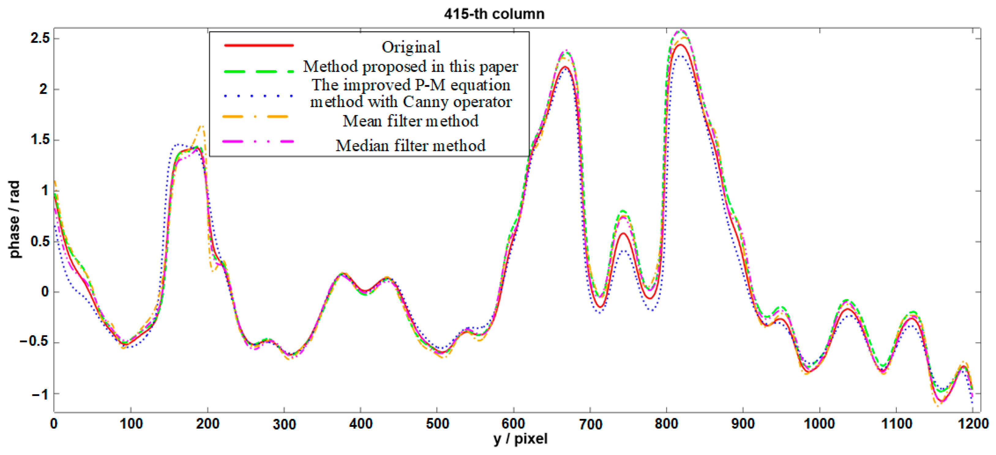
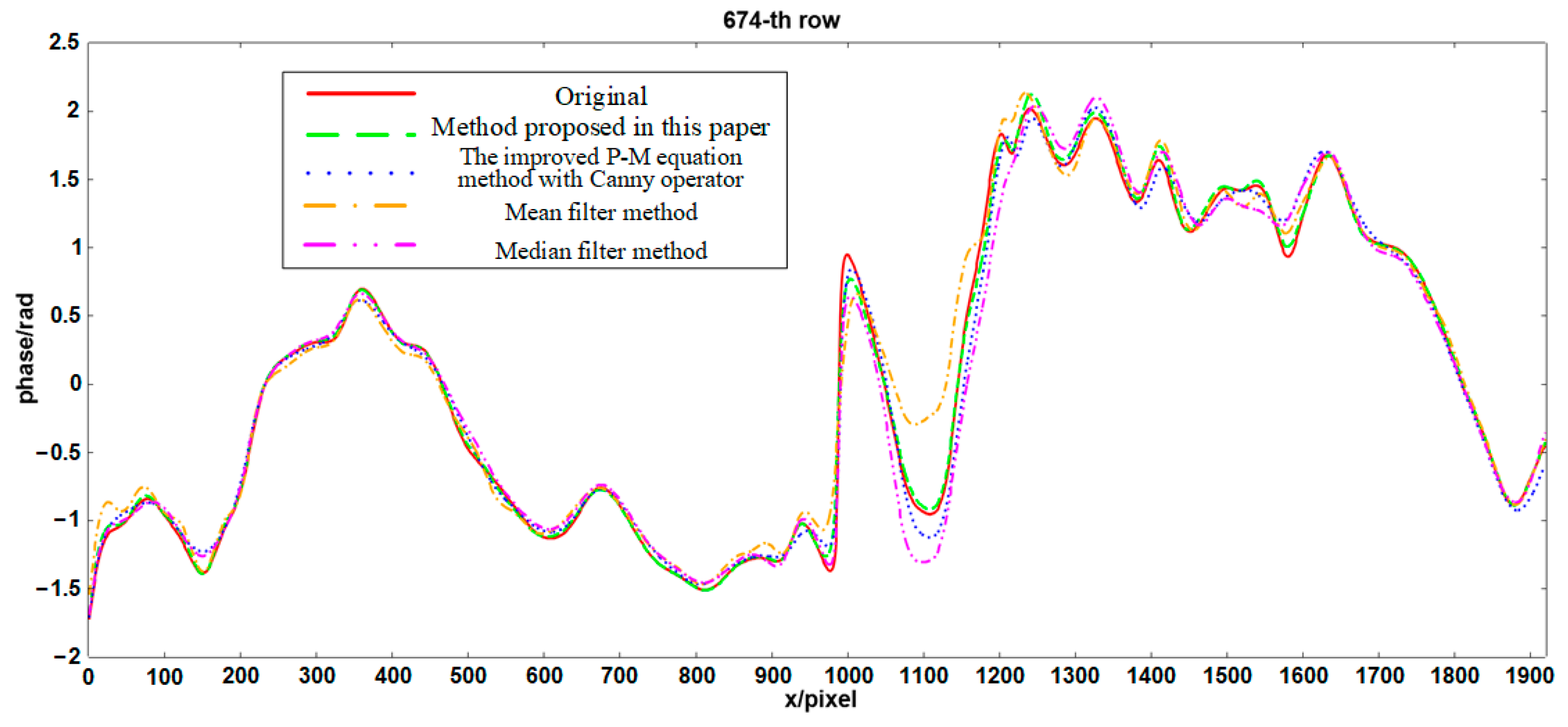
3.4. Phase Cross-Section Curve Analysis

To verify the accuracy of quantitative phase reconstruction after denoising, we performed phase cross-section curve comparison and analysis. The cross-section curve at x = 415 of the phase maps is shown in Figure 7a–d (the red dotted line in Figure 7a) and the original phase map is shown in Figure 9. The cross-section curve at y = 674 of the phase maps is shown in Figure 8a–d) (the red dotted line in Figure 8a) and the original phase map is shown in Figure 10. Among them, the red solid line represents the phase change curve corresponding to the original phase map, which is a relatively real phase with smooth phase distribution obtained by the superimposed averaging method of multiple holograms [44] and is used to evaluate the performance of different speckle noise suppression methods. The green dotted line represents the corresponding phase change curve after processing by the method proposed in this paper, and the blue point represents the corresponding phase change curve after processing by the improved P-M equation method with Canny operator. The orange point line represents the corresponding phase change curve after the mean filter method, and the purple double-point line represents the corresponding phase change curve after the median filter method.

From the change of the phase cross-section curve, the change trends of the green dotted line, the blue point, the orange point line, the purple double-point line and the red solid line are basically the same. However, the deviation between the green dotted line and the red solid line is smaller than the deviation between the blue point, the orange point line, the purple double-point line and the red solid line. The specific deviations are shown in

Table 3. Maximum, minimum and average deviation of the green dotted line, the blue point, the orange point line, the purple double-point line from the red solid line.

Deviation	Sample Plate	Honeybee Foot
Deviation 1	0.4403	0.3014
Deviation 2	0.4653	0.4926
Deviation 3	0.6084	0.8348
Deviation 4	0.4679	0.6768
Deviation 5	0.0000	0.0000
Deviation 6	0.0000	0.0001
Deviation 7	0.0002	0.0001
Deviation 8	0.0001	0.0001
Deviation 9	0.0532	0.0288
Deviation 10	0.0619	0.0672
Deviation 11	0.0716	0.0988
Deviation 12	0.0681	0.0908

. Among them, the maximum deviation of the green dotted line, the blue point, the orange point line and the purple double-point line from the red solid line are deviation 1, deviation 2, deviation 3 and deviation 4, respectively; the minimum deviation of the green dotted line, the blue point, the orange point line, the purple double-point line from the red solid line are deviation 5, deviation 6, deviation 7 and deviation 8, respectively; the average deviation of the green dotted line, the blue point, the orange point line, the purple double-point line from the red solid line are deviation 9, deviation 10, deviation 11 and deviation 12, respectively.

To sum up, in QPI, the method proposed in this paper (combining the Canny operator of EMD to improve the P-M diffusion equation method) has better comparison results of phase cross-section curves than other existing methods. The method proposed in this paper has better speckle noise suppression effect, smaller deviation and higher phase reconstruction accuracy.

4. Discussion

4.1. Error Sources and Analysis

Although the quality of the reconstructed phase map is improved by the method proposed in this paper, the phase reconstruction accuracy may be further improved with other strategies. According to the working mechanism of the interferogram recording system, the main sources of possible phase errors are from: (1) the stability of the light source. The characteristics of the material inside the laser and the temperature increase can cause the power and frequency of the laser to change. This will eventually affect the results of QPI, resulting in inaccurate phase results. (2) The environmental vibration. For Mach–Zehnder interference system, object and reference light waves propagate through different geometric paths and arrive at the CCD recording surface to form an interferogram. Small perturbations such as environmental vibrations can degrade the stability of the interference system. Regarding these issues, we may minimize their influences on phase imaging with a more stable laser in a low and constant temperature in the experiment. A common path off-axis interference system may be introduced to avoid environment vibration. The method proposed in this paper also could be combined with resolution enhancement strategies to obtain accurate high resolution phase map of various applications.

4.2. Improve EMD Speed

Existing EMD can effectively solve the two-dimensional signal decomposition problem, but its high calculation amount still limits its application. It takes about 20 min for EMD to decompose an interferogram with the size of 1920 × 1200 pixels in this paper. In two-dimensional signal EMD process, the main time-consuming steps are the acquisition of extreme points, the construction of extreme surfaces by interpolation and the recursive decomposition. For the acquisition of extreme points, the morphological-based method can be used to replace the statistical method of acquiring extreme point information by traversal, thereby speeding up the calculation speed. For constructing extreme surfaces by interpolation, some fast methods can be used to find the upper and lower envelopes, thereby improving the fitting speed. EMD is a recursive decomposition, so recursion can be optimized to increase the decomposition speed of EMD, for example, by adding some penalty terms. If the speed of EMD is accelerated, the method proposed in this paper can reconstruct the denoised phase map with higher efficiency, which could be applied in the fast inspection on the optical and structure properties of polymeric materials and biomaterials, optical thin-films and glass panels of consumer electronics.

5. Conclusions

In this paper, a speckle noise suppression method combining the Canny operator of EMD to improve the P-M diffusion equation is proposed. This method is used to suppress the influence of speckle noise produced by high-coherence light sources on the phase reconstruction accuracy in QPI. The IMF of high frequency components is obtained by EMD to reconstruct the image with prominent details, which makes the detection of a Canny operator more accurate. Therefore, the diffusion denoising process of the P-M equation is better controlled and high-precision phase information is retained while denoising. In our research, using SSIM, EPI and SSI to quantitatively analyze the reconstructed phase maps after denoising by the method proposed in this paper, the improved P-M equation method with the Canny operator, the mean filter method and the median filter method, the calculation results are better than the other three denoising methods. By analyzing the cross-section curves of the reconstructed phase maps after denoising with different methods, it is found that the proposed method in this paper has a smaller deviation from the original phase. The experimental results show that the method proposed in this paper outperforms the other three denoising methods in performance, with better speckle suppression effect and higher phase reconstruction accuracy.

References

1. Popescu, G. Quantitative Phase Imaging of Cells and Tissues; McGraw-Hill Education: New York, NY, USA, 2011; pp. 121–138. [Google Scholar]
2. Trusiak, M.; Mico, V.; Garcia, J.; Patorski, K. Quantitative phase imaging by single-shot Hilbert–Huang phase microscopy. Opt. Lett. 2016, 41, 4344–4347. [Google Scholar] [CrossRef] [PubMed]
3. Sitthisang, S.; Boonruangkan, J.; Leong, M.F.; Chian, K.S.; Kim, Y.J. Quantitative phase imaging to study the effect of sodium dodecyl surfactant on adherent L929 fibroblasts on tissue culture plates. Photonics 2021, 8, 508. [Google Scholar] [CrossRef]
4. Eldridge, W.J.; Sheinfeld, A.; Rinehart, M.T.; Wax, A. Imaging deformation of adherent cells due to shear stress using quantitative phase imaging. Opt. Lett. 2016, 41, 352–355. [Google Scholar] [CrossRef] [PubMed]
5. Luo, Z.P.; Ma, J.S.; Su, P.; Cao, L.C. Digital holographic phase imaging based on phase iteratively enhanced compressive sensing. Opt. Lett. 2019, 44, 1395–1398. [Google Scholar] [CrossRef]
6. Reddy, B.L.; Ramachandran, P.; Nelleri, A. Compressive complex wave retrieval from a single off-axis digital Fresnel hologram for quantitative phase imaging and microlens characterization. Opt. Commun. 2021, 478, 126371. [Google Scholar] [CrossRef]
7. Zhang, X.; Meng, X.F.; Yin, Y.K.; Yang, X.L.; Wang, Y.R.; Li, X.Y.; Peng, X.; He, W.Q.; Dong, G.Y.; Chen, H.Y. Two-level image authentication by two-step phase-shifting interferometry and compressive sensing. Opt. Lasers Eng. 2018, 100, 118–123. [Google Scholar] [CrossRef]
8. Di, J.L.; Wu, J.; Wang, K.Q.; Tang, J.; Li, Y.; Zhao, J.L. Quantitative phase imaging using deep learning-based holographic microscope. Front. Phys. 2021, 9, 651313. [Google Scholar] [CrossRef]
9. Chen, N.; Wang, C.L.; Heidrich, W. Holographic 3D particle imaging with model-based deep network. IEEE Trans. Comput. Imaging 2021, 7, 288–296. [Google Scholar] [CrossRef]
10. Rivenson, Y.; Liu, T.R.; Wei, Z.S.; Zhang, Y.B.; Haan, K.D.; Ozcan, A. PhaseStain: The digital staining of label-free quantitative phase microscopy images using deep learning. Light Sci. Appl. 2019, 8, 23. [Google Scholar] [CrossRef]
11. Zhang, Y.Y.; Huang, Z.Z.; Jin, S.Z.; Cao, L.C. Autofocusing of in-line holography based on compressive sensing. Opt. Lasers Eng. 2021, 146, 106678. [Google Scholar] [CrossRef]
12. Ren, Z.B.; Lam, E.Y.; Zhao, J.L. Acceleration of autofocusing with improved edge extraction using structure tensor and Schatten norm. Opt. Express 2020, 28, 14712–14728. [Google Scholar] [CrossRef] [PubMed]
13. Guo, C.F.; Bian, Z.C.; Alhudaithy, S.; Jiang, S.W.; Tomizawa, Y.; Song, P.M.; Wang, T.B.; Shao, X.P. Brightfield, fluorescence, and phase-contrast whole slide imaging via dual-LED autofocusing. Biomed. Opt. Express 2021, 12, 4651–4660. [Google Scholar] [CrossRef] [PubMed]
14. Li, R.J.; Cao, L.C. Complex wavefront sensing based on coherent diffraction imaging using vortex modulation. Sci. Rep. 2021, 11, 9019. [Google Scholar] [CrossRef] [PubMed]
15. Ionel, L.; Ursescu, D.; Neagu, L.; Zamfirescu, M. On-site holographic interference method for fast surface topology measurements and reconstruction. Phys. Scr. 2015, 90, 065502. [Google Scholar] [CrossRef]
16. Deng, D.N.; Qu, W.J.; He, W.Q.; Liu, X.L.; Peng, X. Phase aberration compensation for digital holographic microscopy based on geometrical transformations. J. Opt. 2019, 21, 085702. [Google Scholar] [CrossRef]
17. Singh, M.; Khare, K. Accurate efficient carrier estimation for single-shot digital holographic imaging. Opt. Lett. 2016, 41, 4871–4874. [Google Scholar] [CrossRef]
18. Liu, Y.; Wang, Z.; Li, J.S.; Gao, J.M.; Huang, J.H. Total aberrations compensation for misalignment of telecentric arrangement in digital holographic microscopy. Opt. Eng. 2014, 53, 112307. [Google Scholar] [CrossRef]
19. Dong, J.; Jia, S.H.; Yu, H.Q. Hybrid method for speckle noise reduction in digital holography. JOSA A 2019, 36, D14–D22. [Google Scholar] [CrossRef]
20. Monroy, F.; Rincon, O.; Torres, Y.M.; Garcia-Sucerquia, J. Quantitative assessment of lateral resolution improvement in digital holography. Opt. Commun. 2008, 281, 3454–3460. [Google Scholar] [CrossRef]
21. Langehanenberg, P.; Bally, G.V.; Kemper, B. Application of partially coherent light in live cell imaging with digital holographic microscopy. J. Mod. Opt. 2010, 57, 709–717. [Google Scholar] [CrossRef]
22. Choi, Y.; Yang, T.D.; Lee, K.J.; Choi, W. Full-field and single-shot quantitative phase microscopy using dynamic speckle illumination. Opt. Lett. 2011, 36, 2465–2467. [Google Scholar] [CrossRef]
23. Farrokhi, H.; Boonruangkan, J.; Chun, B.J.; Rohith, T.M.; Mishra, A.; Toh, H.T.; Yoon, H.S.; Kim, Y.J. Speckle reduction in quantitative phase imaging by generating spatially incoherent laser field at electroactive optical diffusers. Opt. Express 2017, 25, 10791–10800. [Google Scholar] [CrossRef]
24. Tania, S.; Rowaida, R. A comparative study of various image filtering techniques for removing various noisy pixels in aerial image. Int. J. Signal Process. Image Process. Pattern Recognit. 2016, 9, 113–124. [Google Scholar] [CrossRef]
25. Garcia-Sucerquia, J.; Ramírez, J.A.H.; Prieto, D.V. Reduction of speckle noise in digital holography by using digital image processing. Optik 2005, 116, 44–48. [Google Scholar] [CrossRef]
26. Uzan, A.; Rivenson, Y.; Stern, A. Speckle denoising in digital holography by nonlocal means filtering. Appl. Opt. 2013, 52, A195–A200. [Google Scholar] [CrossRef]
27. Montresor, S.; Tahon, M.; Laurent, A.; Picart, P. Computational denoising based on deep learning for phase data in digital holographic interferometry. APL Photonics 2020, 5, 030802. [Google Scholar] [CrossRef]
28. Niu, R.; Tian, A.L.; Wang, D.S.; Liu, B.C.; Wang, H.J.; Qian, X.T.; Liu, W.G. Speckle noise suppression of digital holography measuring system. Laser Optoelectron. Prog. 2022, 59, 1609002. [Google Scholar]
29. Gao, M.; Kang, B.S.; Feng, X.C.; Zhang, W.; Zhang, W.J. Anisotropic diffusion based multiplicative speckle noise removal. Sensors 2019, 19, 3164. [Google Scholar] [CrossRef]
30. Wu, Y.M.; Duan, H.Y.; Wen, Y.F.; Cheng, H.B.; Wang, T. Study on denoising technology to reproduction image detail. Imag. Sci. Photochem. 2018, 36, 187–191. [Google Scholar]
31. Arsenault, H.H.; April, G. Properties of speckle integrated with a finite aperture and logarithmically transformed. JOSA 1976, 66, 1160–1163. [Google Scholar] [CrossRef]
32. Perona, P.; Malik, J. Scale-space and edge detection using anisotropic diffusion. IEEE Trans. Pattern Anal. Mach. Intell. 1990, 12, 629–639. [Google Scholar] [CrossRef]
33. Yuan, J.J. Improved anisotropic diffusion equation based on new non-local information scheme for image denoising. IET Comput. Vis. 2015, 9, 864–870. [Google Scholar] [CrossRef]
34. Deng, L.Z.; Zhu, H.; Yang, Z.; Li, Y.J. Hessian matrix-based fourth-order anisotropic diffusion filter for image denoising. Opt. Laser Technol. 2019, 110, 184–190. [Google Scholar] [CrossRef]
35. Abdullah Yahya, A.; Tan, J.Q.; Su, B.Y.; Liu, K.; Hadi, A.N. Image edge detection method based on anisotropic diffusion and total variation models. J. Eng. 2019, 2019, 455–460. [Google Scholar] [CrossRef]
36. Anand, A.; Chhaniwal, V.K.; Javidi, B. Real-time digital holographic microscopy for phase contrast 3D imaging of dynamic phenomena. J. Disp. Technol. 2010, 6, 500–505. [Google Scholar] [CrossRef]
37. Wang, F.; Bian, Y.M.; Wang, H.C.; Lyu, M.; Pedrini, G.; Osten, W.; Barbastathis, G.; Situ, G.H. Phase imaging with an untrained neural network. Light Sci. Appl. 2020, 9, 77. [Google Scholar] [CrossRef]
38. Huang, Z.Z.; Cao, L.C. Bicubic interpolation and extrapolation iteration method for high resolution digital holographic reconstruction. Opt. Lasers Eng. 2020, 130, 106090. [Google Scholar] [CrossRef]
39. Ghiglia, D.C.; Romero, L.A. Robust two-dimensional weighted and unweighted phase unwrapping that uses fast transforms and iterative methods. JOSA A 1994, 11, 107–117. [Google Scholar] [CrossRef]
40. Kong, I.B.; Kim, S.W. General algorithm of phase-shifting interferometry by iterative least-squares fitting. Opt. Eng. 1995, 34, 183–188. [Google Scholar] [CrossRef]
41. Hore, A.; Ziou, D. Image quality metrics: PSNR vs.SSIM. In Proceedings of the 2010 20th International Conference on Pattern Recognition, IEEE Computer Society, Istanbul, Turkey, 23–26 August 2010; pp. 2366–2369. [Google Scholar]
42. Soni, V.K.; Soni, P. Wavelet based edge preservation and noise reduction in OCR images. JIST 2022, 12, 127–133. [Google Scholar]
43. Sheng, Y.; Xia, Z.G. A comprehensive evaluation of filters for radar speckle suppression. In Proceedings of the 1996 International Geoscience and Remote Sensing Symposium, IEEE Xplore, Lincoln, NE, USA, 27–31 May 1996; pp. 1559–1561. [Google Scholar]
44. Pan, F.; Xiao, W.; Liu, S.; Wang, F.J.; Rong, L.; Li, R. Coherent noise reduction in digital holographic phase contrast microscopy by slightly shifting object. Opt. Express 2011, 19, 3862–3869. [Google Scholar] [CrossRef]
Figure 1. Solve the gradients in the four directions.
Photonics 09 00611 g001
Figure 2. The flowchart of the method proposed in this paper.
Photonics 09 00611 g002
Figure 3. Schematic diagram and physical diagram of digital recording optical path based on Mach–Zender interferometer. (a) Schematic diagram. (b) Physical diagram.
Photonics 09 00611 g003
Figure 4. Experimental samples and interferograms. (a) Sample plate. (b) The interferogram of (a). (c) Honeybee foot. (d) The interferogram of (c).
Photonics 09 00611 g004
Figure 5. Reconstruction results with different IMF components selected. (a) The first IMF component C 1 of Figure 4b is selected to reconstruct the image. (b) The third IMF component C 3 of Figure 4b is selected to reconstruct the image. (c) The fifth IMF component C 5 of Figure 4b is selected to reconstruct the image. (d) The seventh IMF component C 7 of Figure 4b is selected to reconstruct the image. (e) The first IMF component C 1 of Figure 4d is selected to reconstruct the image. (f) The third IMF component C 3 of Figure 4d is selected to reconstruct the image. (g) The fourth IMF component C 4 of Figure 4d is selected to reconstruct the image. (h) The sixth IMF component C 6 of Figure 4d is selected to reconstruct the image.
Photonics 09 00611 g005
Figure 6. Canny operator edge detection results. (a) The edge detection result of Figure 5a by Canny operator. (b) The edge detection result of Figure 4b by Canny operator. (c) The edge detection result of Figure 5e by Canny operator. (d) The edge detection result of Figure 4d by Canny operator.
Photonics 09 00611 g006
Figure 7. The reconstructed phase maps of sample plate interferogram. (ad) 3D display of the reconstructed phase maps after processing Figure 4b by the method proposed in this paper, the improved P-M equation method with Canny operator, the mean filter method and the median filter method, respectively. (e) The 3D display of the reconstructed phase map of Figure 4b without denoising. (fi) The 2D display of the reconstructed phase maps after processing Figure 4b by the method proposed in this paper, the improved P-M equation method with Canny operator, the mean filter method and the median filter method, respectively. (j) The 2D display of the reconstructed phase map of Figure 4b without denoising.
Photonics 09 00611 g007
Figure 8. The reconstructed phase maps of honeybee foot interferogram. (ad) The 3D display of the reconstructed phase maps after processing Figure 4d by the method proposed in this paper, the improved P-M equation method with Canny operator, the mean filter method and the median filter method, respectively. (e) The 3D display of the reconstructed phase map of Figure 4d without denoising. (fi) The 2D display of the reconstructed phase maps after processing Figure 4d by the method proposed in this paper, the improved P-M equation method with Canny operator, the mean filter method and the median filter method, respectively. (j) The 2D display of the reconstructed phase map of Figure 4d without denoising.
Photonics 09 00611 g008
Figure 9. The cross-section curve at x = 415 of the phase maps shown in Figure 7a–d and the original phase map.
Photonics 09 00611 g009
Figure 10. The cross-section curve at y = 674 of the phase maps shown in Figure 8a–d and the original phase map.
Photonics 09 00611 g010