Article

Range Intensity Profiles of Multi-Slice Integration for Pulsed Laser Range-Gated Imaging System

1
College of Weapons Engineering, Naval University of Engineering, Wuhan 430033, China
2
Naval Petty Officer School, Bengbu 233012, China
3
Shandong Institute of Aerospace Electronic Technology, Yantai 264670, China
*
Author to whom correspondence should be addressed.
Photonics 2022, 9(7), 505; https://doi.org/10.3390/photonics9070505
Submission received: 14 May 2022 / Revised: 10 July 2022 / Accepted: 19 July 2022 / Published: 21 July 2022

Abstract

:
Pulsed laser range-gated imaging (PLRGI) is one of the most effective methods to achieve underwater high-resolution imaging. When searching target, there are two methods can be used: fixed gate and sliding gate. In practice, fixed gate has a small depth of field of view and sliding gate cannot meet the need of real time. In order to overcome these problems, multi-slice integration (MSI) method is proposed in this paper. First, the laser energy received by the PLRGI system is derived from radiative transfer theory. In addition, range intensity profiles (RIP) of MSI method is established. Experiments are carried out in lab to validate the RIP model and results show that theoretical data and experimental data are in good coincidence. Then the gate width and the number of pulse assigned to each slice are discussed. Finally, to prove the effectiveness of the MSI method, experiments are carried out in a boat tank. Results show that the MSI method is better than the fixed gate method for surveillance, and can acquire a clear image of the target at 18 m (4.5 times of the attenuation length) in the water with attenuation coefficient of 0.25 m−1.

1. Introduction

A rapid increasing attention has been paid to the marine development and there is an an urgent need for underwater high-resolution imaging technology [1,2,3,4,5,6]. At present, there are mainly two methods for underwater imaging [7]. One is acoustic imaging and the other is optical imaging. Acoustic imaging can work far away from the target, but it is difficult to achieve high-resolution image. Optical imaging has high resolution, but it is limited by the underwater environment (rapid decay of light energy, impact of backscattered light, etc.) and works at a closer distance [8]. Thus, special optical imaging techniques are needed to overcome the shortcomings, and the pulsed laser range-gated imaging (PLRGI) is one of the effective methods [9,10,11,12].
By controlling the delay time and the gate width (GW), the PLRGI system enables a slice imaging approach similar to that of computed tomography [13]. The delay time determines position of the slice and the GW determines slice width. Traditional PLRGI system can acquire an image from only one slice in one acquisition. Thus, two different strategies are assumed for target searching: fixed gate and sliding gate. System with a single fixed gate can be treated as a conventional camera. System with sliding gate scans the field of view (FOV) with more than one gate positions. An example is shown in Figure 1, T1 and T2 are two targets in the FOV, and T2 is father away from the PLRGI system than T1. Figure 1a shows the example of fixed gate. In order to obtain all the targets in one image frame, the value of GW must be big enough. However, the output image of T2 is much darker than that of T1 because light energy transmitted underwater decays rapidly with increasing distance. Example for sliding gate is shown in Figure 1b. Sliding gate can remove the problem brought by the fixed gate, but take more time to scan the FOV and cannot meet the need of real time performance.
To overcome the problem for searching target, there are two methods can be used. One is multi-channel receivers, which can acquire images from multi-slice at the same time [2,14]. However, this will make the system too complex and expensive. The other one is multi-pulse integration (MPI) method, which split the detection area into multi-areas and assigned pulses to detect each area alone and combined them to a single image [15,16]. However, the model for MPI method is not complete and the number of pulses allocated to each slice is the same in the literature. In addition, this makes it similar to a single slice and suffers from the problem mentioned above.
Inspired by the MPI method, a multi-slice integration (MSI) method is proposed in this work. Different from the MPI method, number of the pulses assigned to each slice and GW of each slice can be different from each other in the proposed MSI method. The paper is organized as follows: following this Introduction section, principles of the traditional PLRGI and MSI method are described and the range intensity profiles (RIP) of the MSI method is established by radiative transfer theory in Section 2. The number of pulse assigned to each slice is determined by the rules that peak energy of each slice are kept as the same. In addition, the best value of GW for every slice is discussed as well. In Section 3, experiments are designed and conducted, and the experimental results are presented and discussed. Conclusions are drawn in the last section.

2. Methods

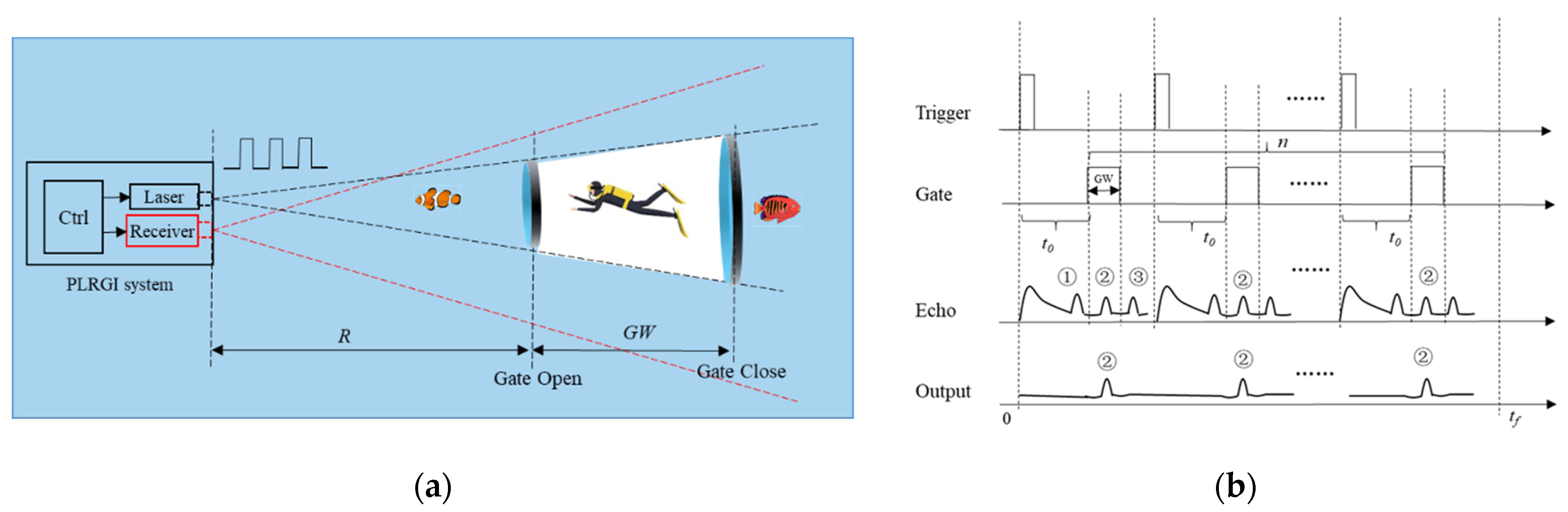
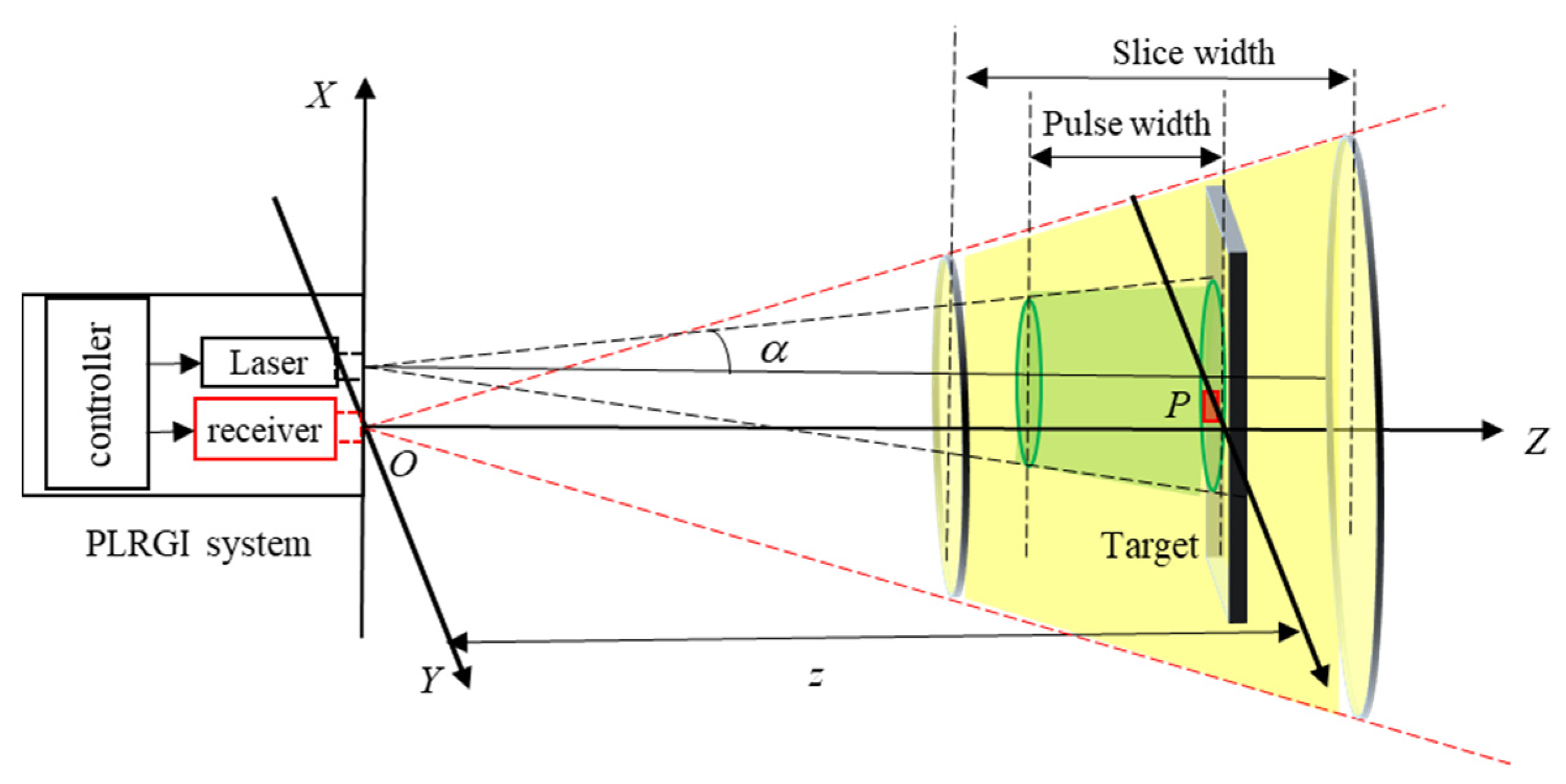
2.1. Principle of PLRGI

Principle of PLRGI is shown in Figure 2. PLRGI system has three main components: a laser, a receiver (camera with a selective gate), and a synchronous controller. When the laser emits a pulse, the controller records the moment and calculates the delay time for the laser to reach the target and return. Before the pulse reaches the camera, the gate is close. In addition, when the pulse reaches the camera, the gate is opened. The opening time for the gate corresponds to the depth of the slice. In this way, the PLRGI system can remove most of the backscattered light.
PLRGI system enables a slice imaging approach similar to that of computed tomography. In addition, information of the slice depends on the delay time, gate width (GW) and the number of pulse assigned to the slice. Position of the slice depends on the delay time and GW. Intensity of the same slice depends on the number of pulse assigned to the slice. Starting position of the slice is calculated by the TOF of the emitted laser pulse, which is written as,
R = 1 2 c w t 0 ,
where cw is the light speed in water and t0 is the delay time.
Let duration of the gate be τ, then width of the slice w is calculated as,
w = 1 2 c w τ .

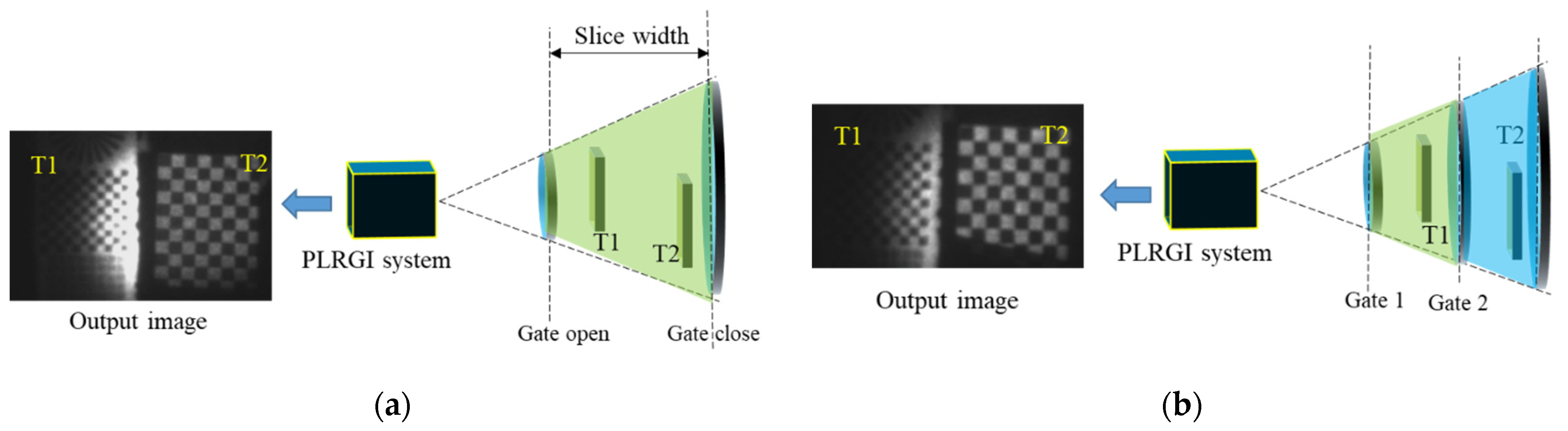
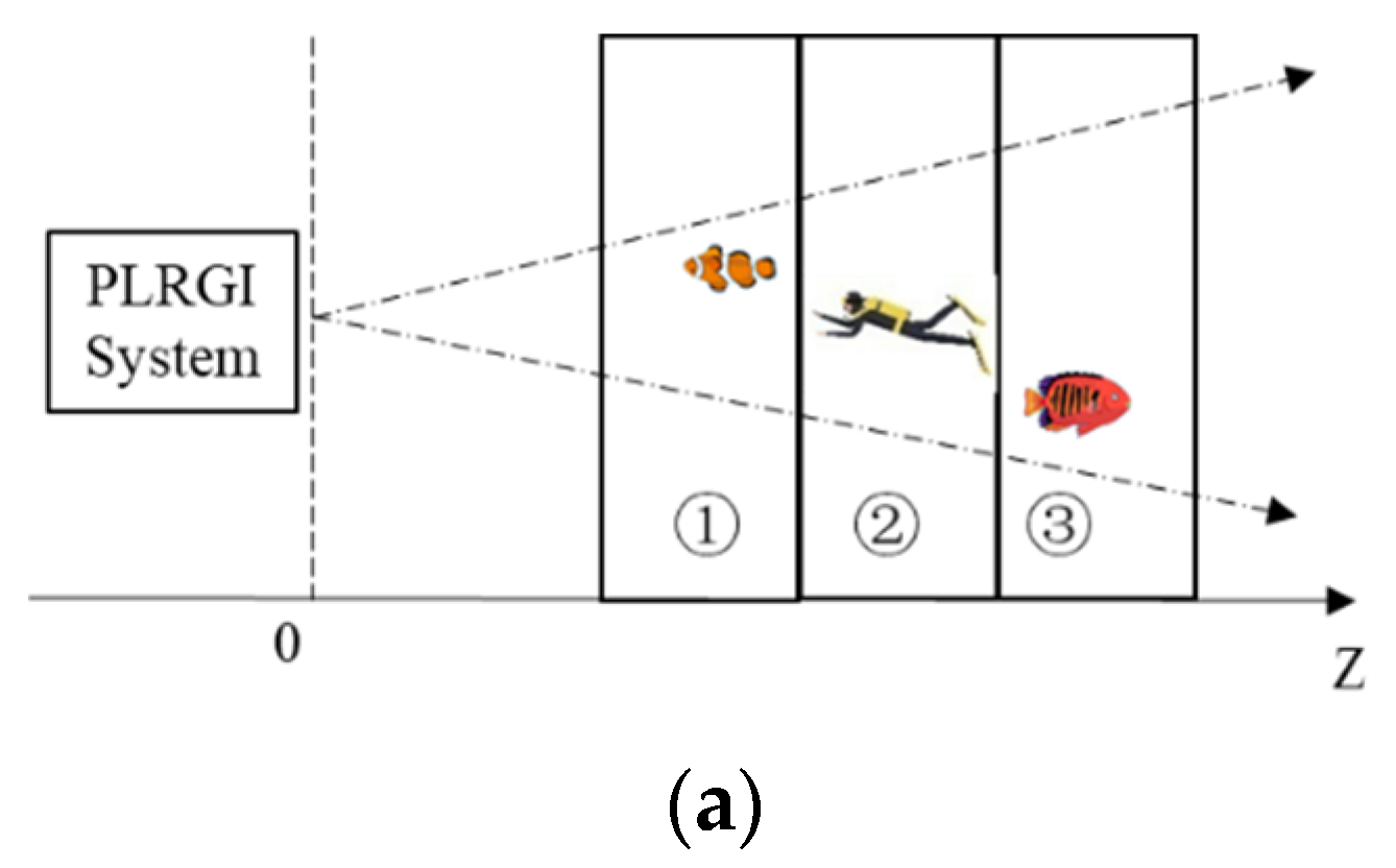
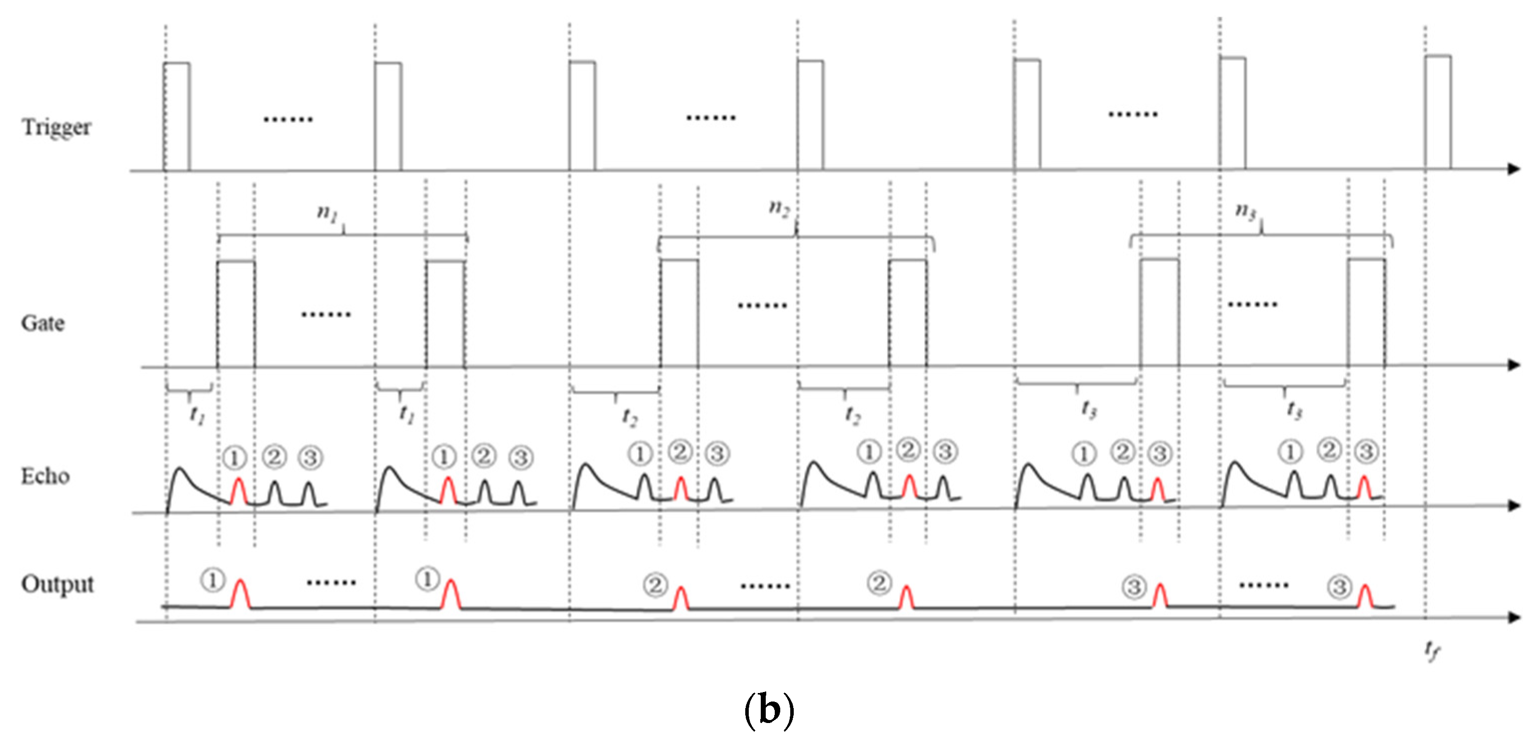
2.2. Multi-Slice Integration Method

Three slices are taken into consideration to present the principle of the MSI method as shown in Figure 3. In the system, a laser with a high pulse repetition frequency is utilized. The laser pulses in a video frame can be split into three groups, and each group corresponds to one slice. Each slice has its delay time and GW.
The time sequence of the MSI method is shown in Figure 3b. The number of pulse assigned to target ①, ② and ③ are n1, n2 and n3, respectively. Delay time of three groups are t1, t2 and t3, which is different from each other. Each pulse has a range intensity profiles (RIP), and pulses belonging to the same group have the same RIPs. Therefore, three sub-RIPs can be integrated into a video frame. With the MSI method, all of the targets in the FOV can be obtained in a video image frame in real time.
Take the slice which contains target ① as an example to calculate the RIP of a single pulse. The coordinate system established is shown in Figure 4. Here α is the half divergence angle of the laser beam. The laser is assumed to emit a pulse of energy E0 within a short period τP. Speed of the laser in water is cw. Target is placed at position z away from the imaging system. In this work, multiple scattering and the influence of ambient light are not considered.
Light intensity within the divergence angle is assumed to be uniformly distributed, then the illumination on the target is:
E P = E 0 e c z τ p π z 2 ( tan α ) 2 ,
where c is the water attenuation coefficient. Let S be a pixel in the FOV at range z. Area of the element S is:
S P = z 2 f 2 S 0 ,
where f is the focal length and S0 is the area of a single pixel of the camera. Radiant flux received by element S is,
Φ S = E P S P = S 0 E 0 τ p π f 2 ( tan α ) 2 e c z .
Assuming that the target is a Lambert reflector, ρ is the reflectivity of the target. According to the Lambert’s law, the intensity of reflection in the normal direction of element S is,
I r = 1 π ρ Φ S .
Under the assumption of paraxial small angle transmission, the radiant flux reaching the receiver is:
Φ = I r e c z Δ Ω
where Δ Ω π D 2 4 z 2 and D is the diameter of the receiver. By substituting Equation (6) into Equation (7), we can acquire,
Φ = H e 2 c z z 2 ,
where H = ρ D 2 E 0 S 0 4 π τ p f 2 ( tan α ) 2 . According to Jens Busck [17], The amount of light energy received by camera can be expressed as,
E ( z ) = Φ ( t 2 z c w ) G ( t t 1 ) d t ,
where Φ is the laser pulse radiant flux that reach the camera, G the gate function, z distance of the target, cw the light speed in water and t1 the delay time of camera gate. Let τ be the opening time of the camera gate, then the gate function can be treated as rectangular function,
G ( t t 1 ) = { 1 0 t t 1 τ 0 e l s e .
Let z 1 = c w t 1 / 2 be the start position of camera gate, then,
E ( z + z 1 ) = 0 τ Φ ( t 2 z c w ) d t ,
where z’ = zz1. By integrating from 0 to τ, a single pulse energy received by camera is,
E ( z + z 1 ) = { ( 2 z c w t 1 + τ P ) Φ , 2 z c w [ τ p , 0 ] τ P Φ , 2 z c w [ 0 , τ τ p ] ( τ + t 1 2 z c w ) Φ , 2 z c w [ τ τ p , τ ] .
Thus, the RIP data of a single pulse can be obtained from Equation (12). In order to verify Equation (12), experiment is carried out in lab. Water attenuation coefficient in the water tank is 0.32/m. The range of interest is from 3 m to 4 m. Delay time t1 and gate time τ are set as 26.7 ns (z1 = 3 m) and 8.9 ns, respectively. RIP data comparison between theory and experiment is shown in Figure 5a.
From Figure 5a, we can see that data in theory and experiment are in good coincidence. In addition, slice width, influenced by the laser pulse width, is expanded from 1m to 1.5 m. In the MSI method, the laser energy received by camera is,
E i n t e g r a t e d = k = 1 3 n k E k ,
where k means kth slice and Ek can be acquired from Equation (12). According to Equations (12) and (13), three parameters, delay time, number of pulse and GW for each slice, need to be set to acquire the RIP data with the MSI method.

2.3. Method to Determine Parameters in MSI Method

Assuming that the range of interest is from z1 to z0, then delay time t1 is,
t 1 = 2 z 1 c w .
Delay time t2 and t3 are,
t 2 = 2 c w ( z 0 z 1 3 + z 1 ) ,
t 3 = 2 c w ( 2 ( z 0 z 1 ) 3 + z 1 ) .
For the number of pulse, we follow the rules that peak energy of each slice are kept as the same. From Equation (12), it can be seen that the peak energy of each slice appear at the distance z1, z2 and z3, whose delay time corresponding to be t1, t2 and t3. Take the 1st and the 2nd slice as an example, peak energy of 1st slice is,
E z 1 = n 1 H e 2 c z 1 z 1 2 .
Peak energy of 2nd slice is,
E z 2 = n 2 H e 2 c z 2 z 2 2 .
To keep peak energy of the 1st and the 2nd slice the same, we can acquire,
E z 1 = E z 2 .
Then the proportion of n1, n2 is,
n 1 n 2 = z 1 2 z 2 2 e 2 c ( z 1 z 2 )
Another experiment is carried out in lab to verify the pulse allocation strategy. The range of interest is from 3 m to 6 m. According to Equations (14)–(16), delay time t1, t2 and t3 are set as 26.7 ns, 35.6 ns and 44.4 ns, respectively. Gate time τ for all slices is 8.9 ns. Image of the 1st slice is appropriate when the number of pulse is 28. Following the peak energy rule, the number of pulse n2 and n3 are set to be 95 and 280. The difference between RIP data in theory and experiment is shown in Figure 5b and they are also in good coincidence. Moreover, comparing to a single slice, the MSI method can extend the maximal range. It can be seen from Figure 5 that the maximal range is extended from 1.5 m to 3.5 m.
Another parameter need to be set is GW. Light energy received by the system at maximal range is chosen to measure the performance of GW. In simulation, delay time t1, t2 and t3 are set as 26.7 ns, 35.6 ns and 44.4 ns, respectively. Gate time τ is changed from 8.9 ns to 44.4 ns. In addition, intensity of the image varies with the change of τ. Tendency of the intensity is shown in Figure 6.
From Figure 6, we can see that intensity increases with GW and the maximum intensity appears firstly when GW is the sum of the range of interest and the laser pulse width. Thus, ideal GW for the MSI method is the sum of the range of interest and the laser pulse width.

3. Results and Discussion

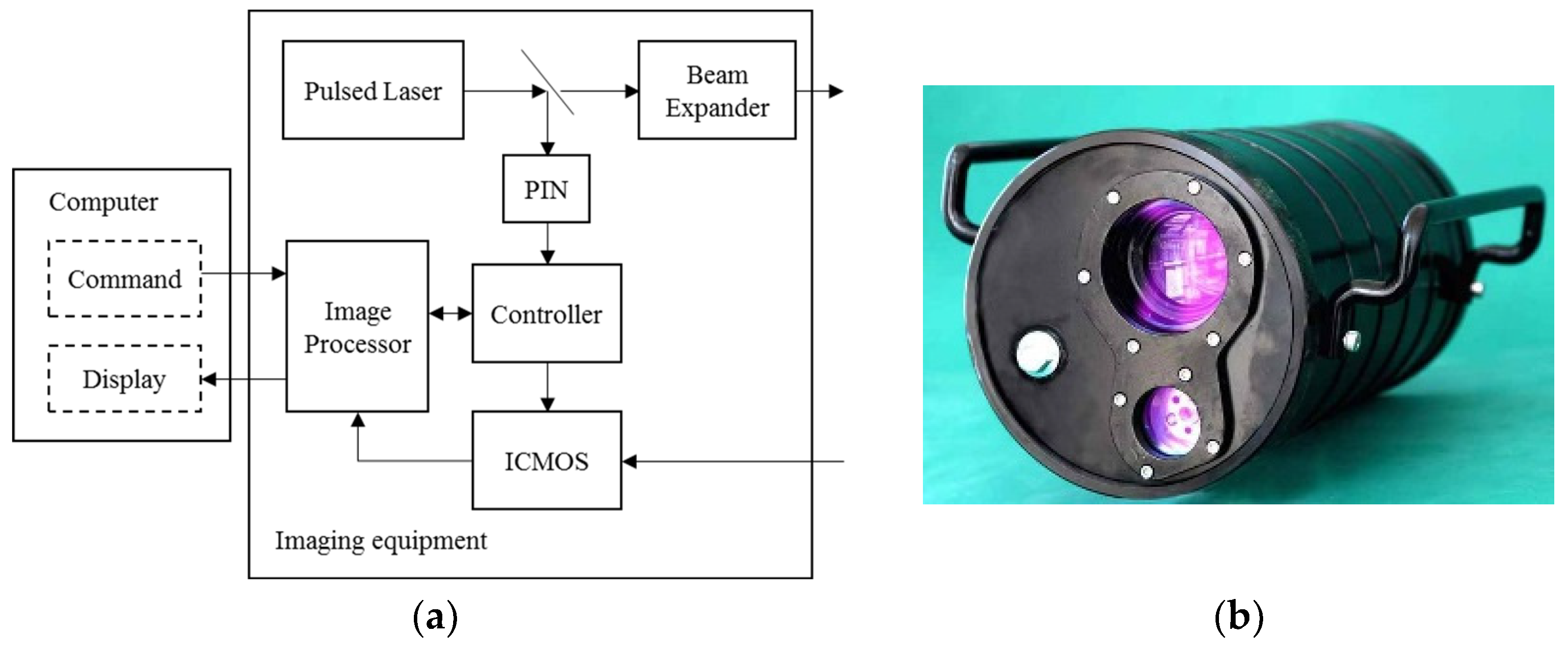
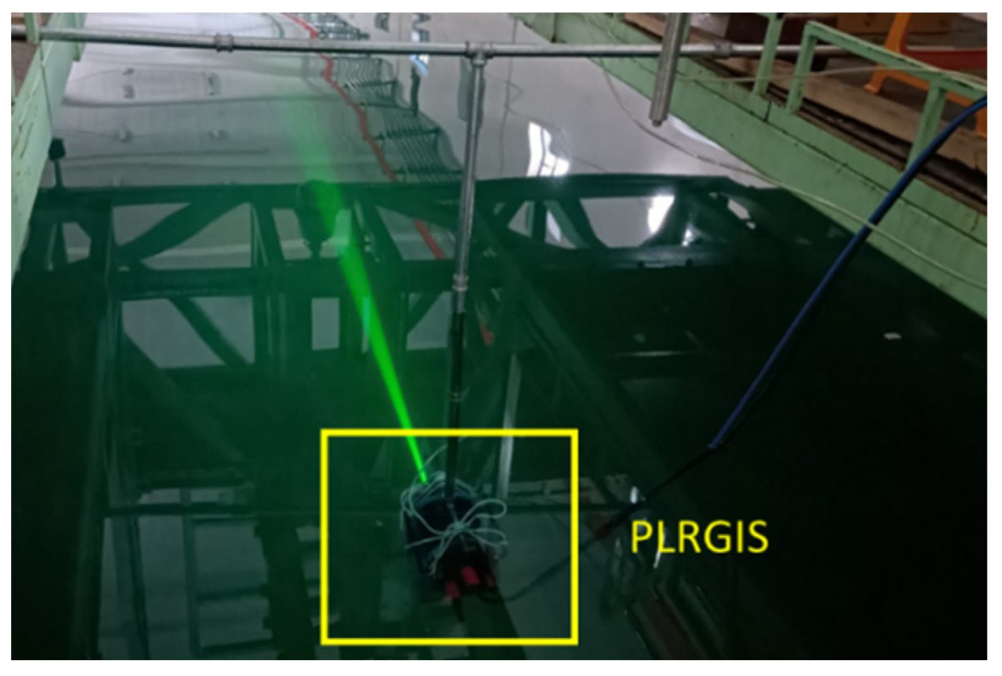
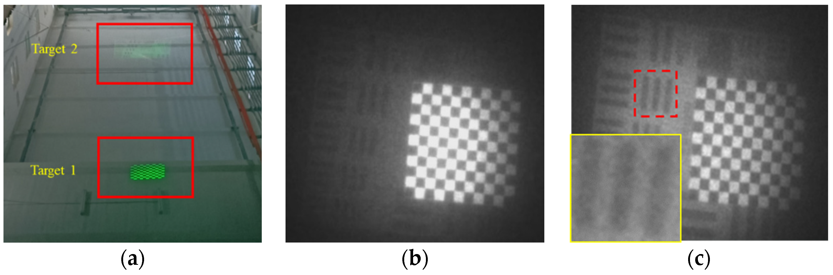
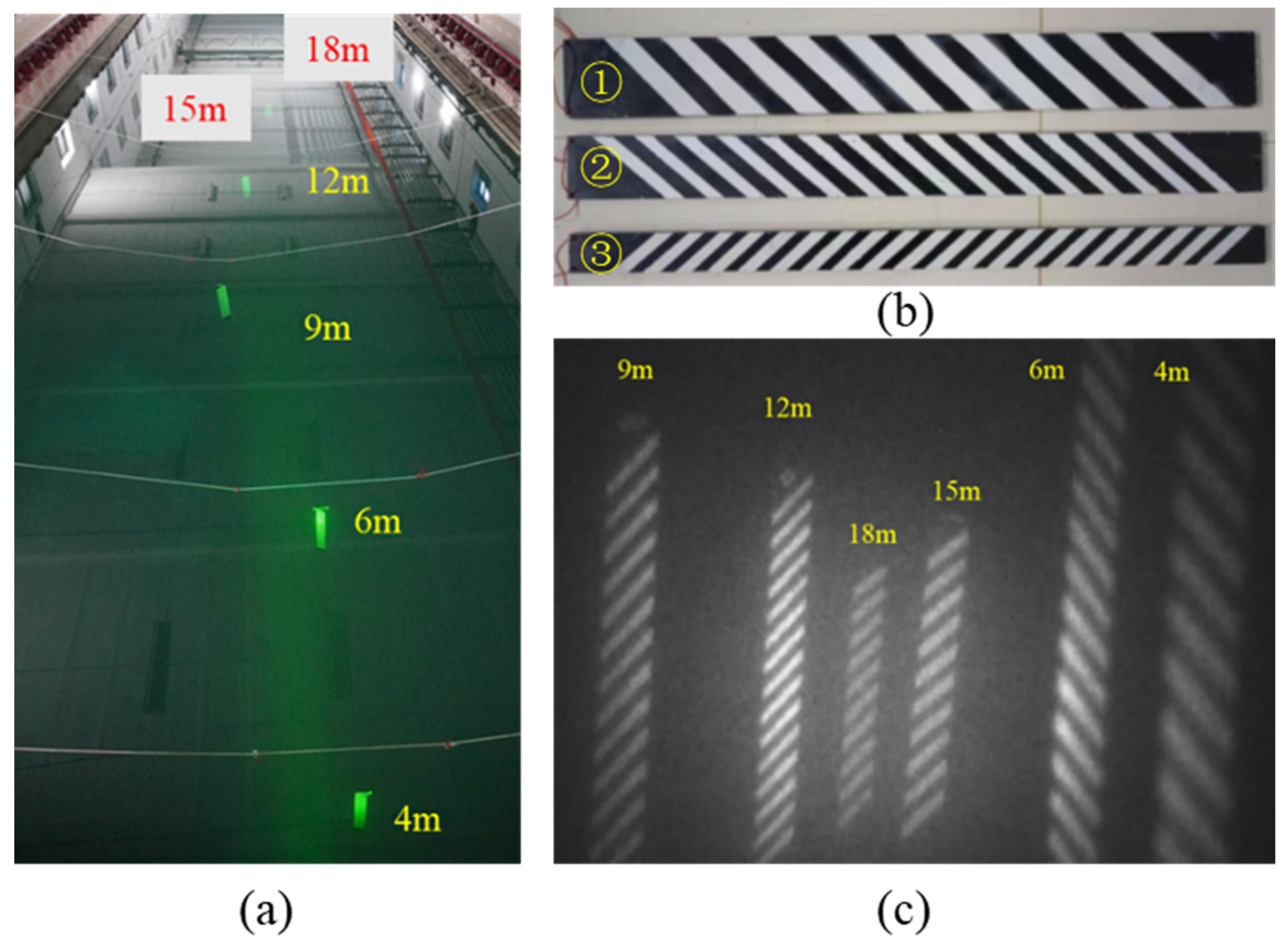
3.1. Experiment Setup

As shown in Figure 7, PLRGI system used in the experiment includes four parts: a pulsed laser, an ICMOS camera, a synchronous controller and an image processor. The laser works at a repetition rate of 10 kHz with a pulse length of 5 ns. In addition, the laser divergence angle can be adjusted when needed. The minimum gate width of the ICMOS is 5 ns. Furthermore, the maximum frame rate is 30 Hz. A FPGA is used for synchronous controlling and a NVIDIA TX2 core module for image processing. The system is controlled by a computer to set its working parameters and to show the imaging result. More information about the system can be acquired from literature [18].
Experiments are carried out in a boat tank, which size is 175 m × 6 m × 4 m (length × width × depth). The wall of the boat tank is rough and the reflectivity of light is low. The PLRGI system is placed at 1m underwater as shown in Figure 8.

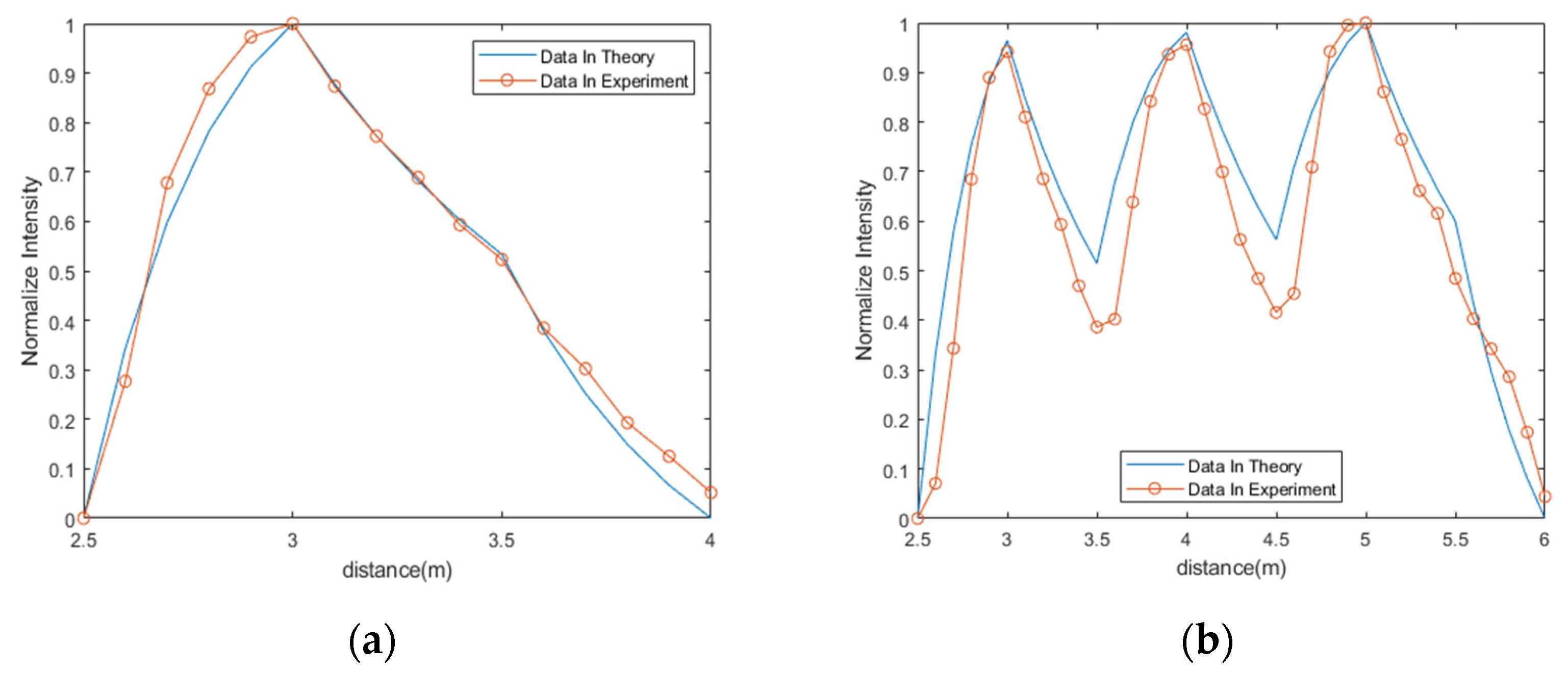
3.2. Comparison of Single Slice and Multi-Slice

Two targets, a resolution target and a checkerboard target, are arranged at 10 m and 15 m directly in front of the system. Size of the resolution target and the checkerboard target are 1 m × 1 m, 0.5 m × 0.5 m, respectively. The albedo for the two regions (black and white) on both targets are 10% and 90%. Range from 10 m to 15 m is the region of interest. Delay time of single slice is 88 ns and GW is 50 ns. For MSI method, the region of interest is split into 3 slices. In addition, delay time of the slices are 88 ns, 103 ns and 117 ns, respectively. GW of all the slices is the same. Furthermore, typical value 25 ns, 43.75 ns and 50 ns are adopted to measure performance of the system. Water attenuation coefficient is estimated to 0.25/m by the method we proposed in literature [19]. So the number of pulse n1, n2 and n3 are set to be 36, 108 and 310. Output of the single slice and MSI method are shown in Figure 9.
Output of single slice shows that target 2 is much darker than that of target 1 because light decays rapidly underwater with increasing distance. Output of MSI method are much better than single slice. Furthermore, in all three MSI method, GW of 50 ns is the best.
To evaluate the quality of the image, intensity and gradient are used as metrics in this paper. The gradient is a metric used to indicate sharpness of an image, and the larger its value, the higher sharpness of the image obtained. We can acquire gradient G from Equation (21),
G = 1 M × N Σ i = 1 M Σ j = 1 N ( f x ) 2 + ( f y ) 2 2
where M, N represent the number of columns and rows of the image.
Metric of intensity is the mean intensity of the area within red dotted lines. It can be expressed as,
M I = 1 M × N Σ i = 1 M Σ j = 1 N I ( i , j )
Quantified comparisons between Figure 9c–f are shown in Figure 10.
It can be seen from Figure 10 that performance of intensity and gradient increase with GW. When GW larger than 50 ns, which is almost the sum of range of interest and laser pulse width, there are not much change in intensity and gradient. This is in good agreement with conclusion in Section 2.

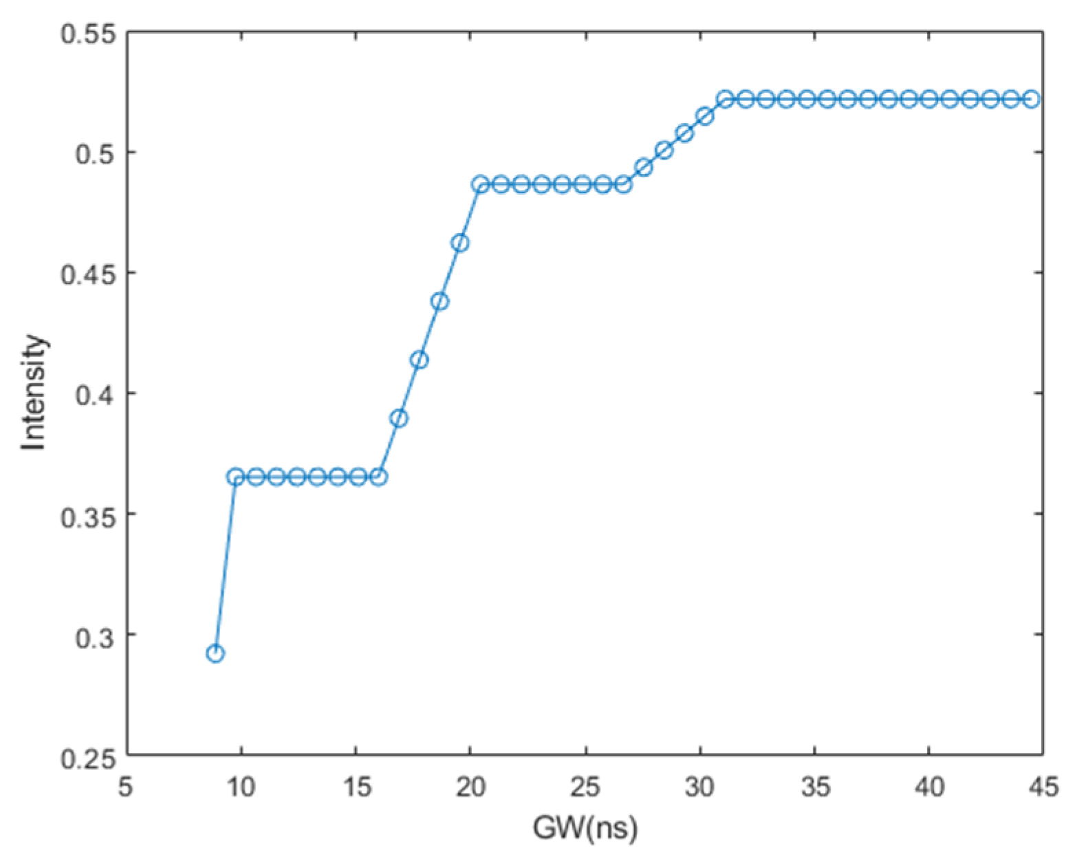
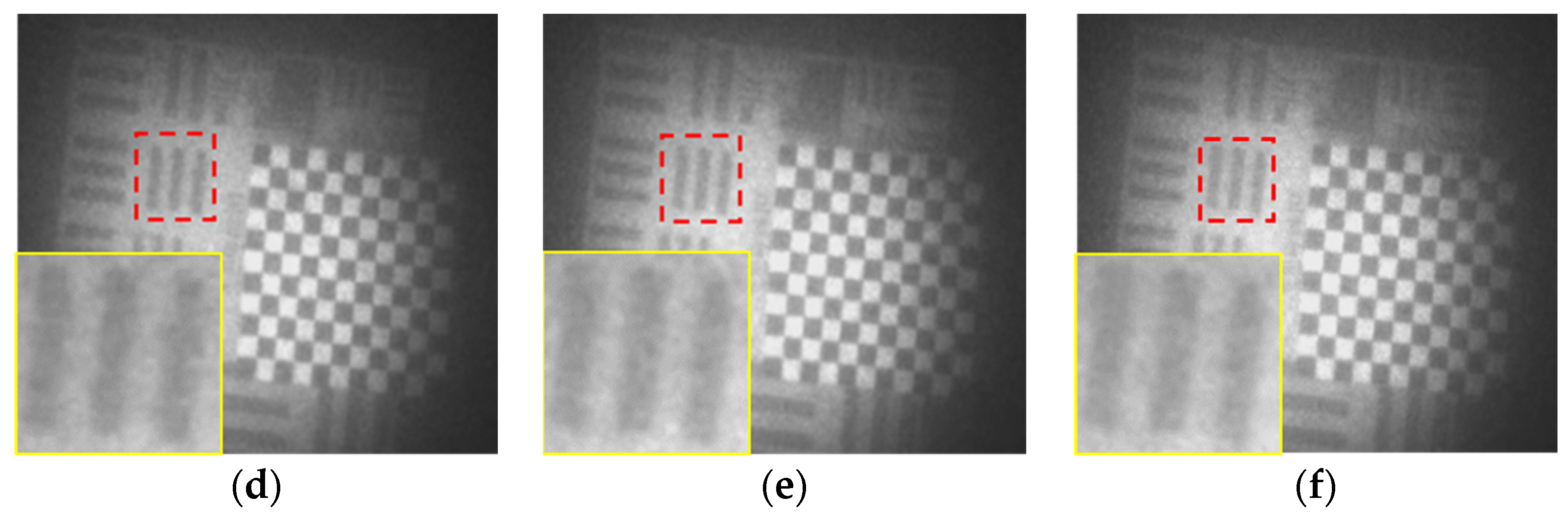
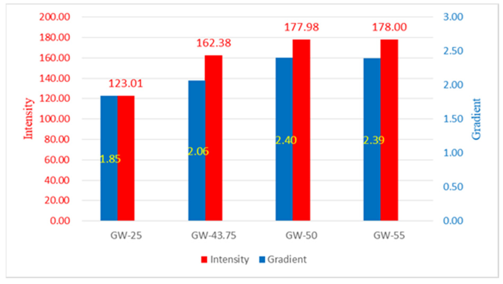
3.3. Performance of MSI Method

To test the performance of MSI method, another experiment is carried out. As shown in Figure 11, we placed 6 targets within the FOV, whose distance are 4 m, 6 m, 9 m, 12 m, 15 m and 18 m, respectively. There are three different sizes of targets: size of ① is 0.1 m × 0.8 m, size of ② is 0.08 m × 0.8 m and size of ③ is 0.05 m × 0.8 m. Two targets of ③ are placed at 4 m and 6 m. Two targets of ② are placed at 9 m and 12 m. Two targets of ① are placed at 15 m and 18 m. The albedo for the two regions (black and white) on all targets are 10% and 90%.
In the experiment, 6 slices are used in MSI method. Delay time of 6 slices are 26.7 ns, 53.3 ns, 80.1 ns, 106.6 ns, 133.3 ns and 160 ns. GW of all the slices are 160 ns. According to Section 2, the number of pulse assigned to each slice are 1, 4, 36, 288, 2000 and 13,018. However, total number of pulse can be assigned is 2500 at video frame of 4 fps. So the number of the pulse assigned to each slice are 1, 4, 36, 288, 2000 and 171.
As shown in Figure 11, all the targets can be seen in the output image and the farthest target at 18 m is distinguishable. Thus, the maximal range of identification for MSI method can reach at least 4.5 attenuation length while that is 2–3 attenuation length for conventional camera system [8,20,21].

4. Conclusions

It can be seen from this paper that there are two methods for searching target in traditional PLRGI system: fixed gate and sliding gate. System with fixed gate has a short visible range. While system with sliding gate takes much time to scan the FOV. To make PLRGI system more suitable for surveillance, two methods are proposed. One is multi-channel, and the other is multi-pulse integration (MPI). However, both methods have shortcomings. This paper reports our multi-slice integration (MSI) method to solve the problems encountered above.
Different from MPI method, number of the pulses assigned to each slice and GW of each slice can be different from each other in MSI method. RIP of MSI method is established by radiative transfer theory. In addition, experiments carried out in lab prove that the RIP is correct. Then we follow the rules that peak energy of each slice are kept as the same to determine the number of pulse assigned to each slice. Furthermore, another experiment is carried out to verify the pulse allocation strategy. Next, the best value of GW for every slice is discussed. The results of simulation and experiments show that the best value of GW for MSI method is the sum of range of interest and laser pulse width. Lastly, experiments carried out in the boat tank show that MSI method is effective for PLRGI system, and the performance range for MSI method can reach at least 4.5 attenuation length.

Author Contributions

All experiments were carried out and analyzed by all authors. H.L. wrote the manuscript, which was discussed by all authors. All authors have read and agreed to the published version of the manuscript.

Funding

This research received no external funding.

Institutional Review Board Statement

Not applicable.

Informed Consent Statement

Not applicable.

Data Availability Statement

The data that support this study are proprietary in nature and may only be provided with restrictions.

Acknowledgments

The authors thank Huazhong University of Science and Technology for the support of experiment in the boat tank. The authors thank Zhang Su, Kai Li and Sun Chunsheng for the help during the experiment.

Conflicts of Interest

The authors declare no conflict of interest.

References

  1. Weidemann, A.; Fournier, G.R.; Forand, L.; Mathieu, P. In Harbor Underwater Threat Detection/Identification Using Active Imaging. In Proceedings of the Photonics for Port and Harbor Security, Orlando, FL, USA, 19 May 2005; SPIE: Orlando, FL, USA, 2005; Volume 5780, pp. 59–70. [Google Scholar]
  2. Ulich, B.L.; Lacovara, P.; Moran, S.E.; DeWeert, M.J. Recent Results in Imaging Lidar. In Proceedings of the Advances in Laser Remote Sensing for Terrestrial and Oceanographic Applications, Orlando, FL, USA, 2 July 1997; SPIE: Orlando, FL, USA, 2005; Volume 3059, pp. 95–108. [Google Scholar]
  3. Matsumoto, N. Development of Underwater Search and Rescue Remotely Operated Vehicles. Adv. Robot. 2002, 16, 561–564. [Google Scholar] [CrossRef]
  4. A.Mol’kov, A.; S.Dolin, L. The Possibility of Determining Optical Properties of Water from the Image of the Underwater Solar Path. Radiophys. Quantum 2016, 58, 586–597. [Google Scholar] [CrossRef]
  5. Mariani, P.; Quincoces, I.; Haugholt, K.H.; Chardard, Y.; Visser, A.W.; Yates, C.; Piccinno, G.; Reali, G.; Risholm, P.; Thielemann, J.T. Range-Gated Imaging System for Underwater Monitoring in Ocean Environment. Sustainability 2018, 11, 162. [Google Scholar] [CrossRef] [Green Version]
  6. Yang, K.; Yu, L.; Xia, M.; Xu, T.; Li, W. Nonlinear RANSAC with Crossline Correction: An Algorithm for Vision-Based Curved Cable Detection System. Opt. Lasers Eng. 2021, 141, 106417. [Google Scholar] [CrossRef]
  7. Shen, Y.; Zhao, C.; Liu, Y.; Wang, S.; Huang, F. Underwater Optical Imaging: Key Technologies and Applications Review. IEEE Access 2021, 9, 85500–85514. [Google Scholar] [CrossRef]
  8. Dalgleish, F.R.; Vuorenkoski, A.K.; Ouyang, B. Extended-Range Undersea Laser Imaging: Current Research Status and a Glimpse at Future Technologies. Mar. Technol. Soc. J. 2013, 47, 128–147. [Google Scholar] [CrossRef]
  9. Heckman, P.; Hodgson, R. Underwater Optical Range Gating. IEEE J. Quantum Electron. 1967, 3, 445–448. [Google Scholar] [CrossRef]
  10. Tan, C.S.; Sluzek, A.; Seet, G.L.G.; Jiang, T.Y. Range Gated Imaging System for Underwater Robotic Vehicle. In Proceedings of the OCEANS 2006—Asia Pacific, Singapore, Singapore, 16–19 May 2006; IEEE: Manhattan, NY, USA, 2006; pp. 1–6. [Google Scholar]
  11. Jin, W.; Cao, F.; Wang, X.; Liu, G.; Huang, Y.; Qi, H.; Shen, F. Range-Gated Underwater Laser Imaging System Based on Intensified Gate Imaging Technology. In Proceedings of the International Symposium on Photoelectronic Detection and Imaging 2007: Photoelectronic Imaging and Detection, Beijing, China, 25 February 2008; Zhou, L., Ed.; SPIE: Bellingham, WA, USA, 2008; p. 66210L. [Google Scholar]
  12. Jaffe, J.S. Underwater Optical Imaging: The Past, the Present, and the Prospects. IEEE J. Ocean. Eng. 2015, 40, 683–700. [Google Scholar] [CrossRef]
  13. De Dominicis, L. Underwater 3D Vision, Ranging and Range Gating. In Subsea Optics and Imaging; Watson, J., Zielinski, O., Eds.; Woodhead Publishing Series in Electronic and Optical Materials; Woodhead Publishing: Sawston, UK, 2013; pp. 379–410e. ISBN 978-0-85709-341-7. [Google Scholar]
  14. McLean, E.A.; Burris, H.R.; Strand, M.P. Short-Pulse Range-Gated Optical Imaging in Turbid Water. Appl. Opt. AO 1995, 34, 4343–4351. [Google Scholar] [CrossRef]
  15. Acharekar, M.A. Underwater Laser Imaging System (ULIS). In Proceedings of the Detection and Remediation Technologies for Mines and Minelike Targets II, Orlando, FL, USA, 22 July 1997; Dubey, A.C., Barnard, R.L., Eds.; SPIE: Bellingham, WA, USA, 1997; pp. 750–761. [Google Scholar]
  16. Xinwei, W.; Youfu, L.; Yan, Z. Multi-Pulse Time Delay Integration Method for Flexible 3D Super-Resolution Range-Gated Imaging. Opt. Express OE 2015, 23, 7820–7831. [Google Scholar] [CrossRef] [PubMed]
  17. Busck, J. Underwater 3-D Optical Imaging with a Gated Viewing Laser Radar. Opt. Eng 2005, 44, 116001. [Google Scholar] [CrossRef]
  18. Peng, B.; Jin, D.; Ji, C.; Pei, C.; Sun, L. An Underwater Laser Three-Dimensional Imaging System. In Proceedings of the Sixth Symposium on Novel Optoelectronic Detection Technology and Applications, 17 April 2020; SPIE: Bellingham, WA, USA, 2020; Volume 11455, pp. 437–442. [Google Scholar]
  19. Lin, H.; Zhang, X.; Ma, L.; Hu, Q.; Jin, D. Estimation of Water Attenuation Coefficient Byimaging Modeling of the Backscattered Lightwith the Pulsed Laser Range-Gated Imagingsystem. Opt. Contin. 2022, 1, 989–1002. [Google Scholar] [CrossRef]
  20. Jaffe, J.S. Computer Modeling and the Design of Optimal Underwater Imaging Systems. IEEE J. Ocean. Eng. 1990, 15, 101–111. [Google Scholar] [CrossRef]
  21. Forand, J.L.; Fournier, G.R.; Bonnier, D.; Pace, P. LUCIE: A Laser Underwater Camera Image Enhancer. In Proceedings of the OCEANS ’93, Victoria, BC, Canada, 18–21 October 1993; IEEE: Victoria, BC, Canada, 1993; pp. III/187–III/190. [Google Scholar]
Figure 1. Examples of fixed gate and sliding gate. (a) Description of output image from fixed gate; (b) Description of output image from sliding gate.
Photonics 09 00505 g001
Figure 2. Description and Time sequence of the single slice. (a) Principle of PLRGI; (b) Time sequence of the single slice.
Photonics 09 00505 g002
Figure 3. Description and Time sequence of the MSI method with three slices. (a) The three targets are in three adjacent slices respectively; (b) Time sequence of the MSI method. The same delay time belongs to the same slice, and the slice width is small and only one target echo can be passed.
Photonics 09 00505 g003aPhotonics 09 00505 g003b
Figure 4. Coordinate system of PLRGI system.
Photonics 09 00505 g004
Figure 5. RIP data comparison between theory and experiment. (a) RIP of a single pulse; (b) RIP of MSI method.
Photonics 09 00505 g005
Figure 6. Intensity of the maximal range (6 m) varying with GW.
Photonics 09 00505 g006
Figure 7. Component of PLRGI equipment. (a) Principle of the system; (b) Front view of the system.
Photonics 09 00505 g007
Figure 8. Experiment site. PLRGI system is placed at 1 m underwater.
Photonics 09 00505 g008
Figure 9. Performance of single slice and multi-slice. (a) Two targets in experiment; (b) Output of single slice; (c) Output of multi-slice, whose GW is 25 ns; (d) Output of multi-slice, whose GW is 43.75 ns; (e) Output of multi-slice, whose GW is 50 ns; (f) Output of multi-slice, whose GW is 55 ns.
Photonics 09 00505 g009aPhotonics 09 00505 g009b
Figure 10. Performance of different GW in MSI method.
Photonics 09 00505 g010
Figure 11. Experiment in MSI method. (a) Six targets in experiment; (b) Three different sizes of targets; (c) Output image of the system.
Photonics 09 00505 g011
Publisher’s Note: MDPI stays neutral with regard to jurisdictional claims in published maps and institutional affiliations.

