Propagation Characteristics of Hermite–Gaussian Beam under Pointing Error in Free Space

Abstract

Hermite–Gaussian (HG) beams have significant potential to improve the capacity of free-space optical communication (FSOC). The influence of pointing error on the propagation characteristics of an HG beam cannot be ignored in the FSOC system. Although the average irradiance of the HG beam under a small pointing error from the FSOC tracking mechanism has been investigated through Taylor series approximation, here, we propose that the average irradiance of the HG beam under an arbitrary magnitude pointing error can be deduced through a statistical averaging method. We firstly found that the average irradiance profile of an HG beam finally changes into an approximately Gaussian shape with the increase in pointing error and propagation distance and a larger beam waist at the transmitter could mitigate the profile change. The correlation coefficient between deduced theoretical expression and Monte Carlo simulation reaches 0.999. Additionally, the effective spot size, location of the local extreme value, average received power and signal-to-noise ratio (SNR) loss for an HG beam under pointing error were theoretically deduced and analyzed for the first time. We found that the effective spot size of the higher-order HG beam experiences less broadening under the pointing error than that of the lower-order HG beam. The fundamental theoretical expressions of average irradiance for an HG beam under pointing error have provided effective guidance for analyzing the propagation characteristics and link performance.

1. Introduction

Free-space optical communication (FSOC) has the advantages of high bandwidth, high data rate, low energy consumption and high confidentiality and is considered a promising technology for next-generation communication [1,2,3,4].

A Hermite–Gaussian (HG) beam, as a type of higher-order TEM_mn mode Gaussian beam, can be generated using higher-order solutions of the paraxial equation with Hermite polynomials (CO₂ laser) in rectangular coordinates [5]. A higher-order HG beam can form a multiple-spot pattern for the irradiance rather than a single spot as generated by lowest-order Gaussian beam, and furthermore, the HG beam has unique orthogonal spatial modes and well-preserved irradiance distribution in free-space propagation [5,6,7,8,9,10]. The definition of the HG beam’s spot size is different from that of the Gaussian beam which was proposed by Carter [11]. For FSOC system application, the HG beam has garnered attention due to its potential to improve the capacity using mode-division multiplexing (MDM) [12,13,14,15]. Meanwhile, the HG beam can be also used in FSOC with a single-input multiple-output (SIMO) system owing to its propagation characteristics. Therefore, research on the propagation characteristics and expressions of HG beams, which include average irradiance, spot size and location of the local extreme value in the average irradiance for the HG beam, is critical for HG beam applications in FSOC.

Notably, the mobile FSOC link must be maintained by the beam-tracking mechanism, and the pointing error comes from its photoelectric detector noise and platform vibration residual noise which cause the propagation characteristics and irradiance distribution to be different from previous research [16,17,18]. Hence, the pointing error of the beam-tracking mechanism inevitably influences the irradiance distribution, which is one of the most critical characteristics of an HG beam. Kiasaleh first studied the influence of small pointing error (approximately 2.5 μrad with 3000 m) on the average irradiance distribution in free space through a Taylor series approximation [8]. However, the expression of the average irradiance under a small pointing error might become inaccurate as the pointing error increases. Due to the different application requirements of FSOC link systems, different pieces of equipment are selected as the coarse pointing and fine pointing systems. The magnitudes of pointing error are equal to several microradians (μrad) to several tens of microradians (μrad) [4], and a general expression for arbitrary magnitude pointing error is needed.

In this paper, we adopted the statistical averaging method instead of Taylor series approximation to deduce the expression of average irradiance for an HG beam under arbitrary pointing error. Based on average irradiance, the propagation characteristics, average received power and signal-to-noise ratio (SNR) loss of an HG beam have been investigated.

The paper is organized as follows: In Section 2, the statistical averaging method is adopted to establish the modeling of the average irradiance for the HG beam under pointing error. In Section 3, Monte Carlo simulation is used to verify the results of the deduced theoretical expression and prove its accuracy. In Section 4, based on average irradiance, the effective spot size, location of local extreme values in the average irradiance, average received power and signal-to-noise ratio (SNR) loss are discussed. Finally, the conclusions are presented in Section 5.

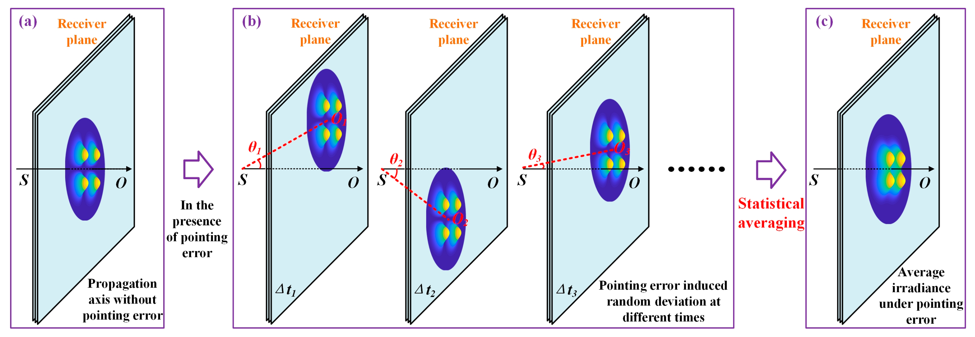
2. Modeling of the Average Irradiance under Pointing Error

The irradiance of a higher-order TEM_mn HG beam can be treated as a generalized eigenfunction of the optical field equation in free space, which is obtained as follows [5,8]:

$$\begin{array}{cc}{I}_{mn}(x,y,L)\hfill & =I_m(x,L)\times I_n(y,L)\hfill \\ & =\frac{W_0^2}{W^2}{H}_m^2\left(\frac{\sqrt{2}x}{W}\right)H_n^2\left(\frac{\sqrt{2}y}{W}\right)\exp \left[-\frac{2(x^2+y^2)}{W^2}\right],\hfill \end{array}$$

(1)

where (x, y) denotes the Cartesian coordinates at distance L; x and y represent the horizontal and vertical directions, respectively; and $H_m(x)$ is a Hermite polynomial of the order m. In particular, for m = n = 0, the HG beam is reduced to the lowest-order TEM₀₀ Gaussian beam. Additionally, W₀ denotes the TEM₀₀ beam waist at the transmitter, and W denotes the TEM₀₀ spot size at the receiver, which is $W=W_0\sqrt{1+{\mathsf{\Lambda }}_0^2}$, where ${\mathsf{\Lambda }}_0=2L/(k{W}_0^2)$, $k=2\pi /\lambda$ denotes the optical wave number and $\lambda$ is the wavelength. Owing to the orthogonal spatial modes of the HG beam, its irradiance in Equation (1) allows for splitting into the horizontal (x-coordinate) and vertical (y-coordinate) direction components [5,6,7,8,9,10], and we observe the following: $I_m(x,L)=\frac{W_0}{W}{H}_m^2\left(\frac{\sqrt{2}x}{W}\right)\exp \left[-\frac{2x^2}{W^2}\right]$ and $I_n(y,L)=\frac{W_0}{W}{H}_n^2\left(\frac{\sqrt{2}y}{W}\right)\exp \left[-\frac{2y^2}{W^2}\right]$.

As shown in Figure 1, the pointing error causes the center of the HG beam to move randomly at the receiving plane. For convenience, a TEM₁₁ HG beam was selected to illustrate this process. The term S denotes the center of the HG beam at the transmitter, and O denotes the center of the receiver plane. The term SO denotes the propagation axis without pointing error (Figure 1a). The center of the HG beam moves to position O_j under the pointing error angle θ_j at time Δt_j, and the cases of j = 1, 2 and 3 are shown in Figure 1b. The term SO_j (j = 1, 2, 3, …) denotes the propagation direction under the pointing error, and θ_j denotes the pointing error angle between SO_j and SO. The average irradiance under the pointing error can be obtained by statistically averaging multiple HG beams at different positions (Figure 1c). Because the probability of appearance at a specific position is determined by the probability density function (PDF) of the pointing error angle, the statistical averaging results can be formulated through position probability weighting for the HG beam irradiance at different positions (see Figure 1c).

The pointing error angle can be generally composed of two independent random variables along the horizontal and vertical axes, and the PDF of the pointing error angle for both the horizontal and vertical axes follows a nonzero-mean Gaussian distribution [5,15]. The pointing error-induced displacement is the product of the pointing error angle and propagation distance, which also follows a zero-mean Gaussian distribution for both the horizontal and vertical axes as follows [5,16,17]:

$$f(r_x)=\frac{1}{\sqrt{2\pi }{\sigma }_r}\exp \left(\frac{-r_x{}^2}{2{\sigma }_r^2}\right),$$

(2)

$$f(r_y)=\frac{1}{\sqrt{2\pi }{\sigma }_r}\exp \left(\frac{-r_y{}^2}{2{\sigma }_r^2}\right),$$

(3)

where $r_x={\theta }_{x}L$ and $r_y={\theta }_{y}L$ denote displacements along the horizontal and vertical axes, respectively, and ${\theta }_x$ and ${\theta }_y$ represent the pointing error angles along the horizontal and vertical directions, respectively. Correspondingly, ${\sigma }_r={\sigma }_{\theta }L$ denotes the standard variance of $r_x$ and $r_y$, and ${\sigma }_{\theta }$ represents the standard variance of ${\theta }_x$ and ${\theta }_y$.

Then, the statistical averaging results for multiple HG beams at different positions can be expressed as follows:

$${\langle I_{mn}(x,y,L)\rangle }_{PE}={\displaystyle {\int }_{-\infty }^{\infty }{\displaystyle {\int }_{-\infty }^{\infty }{I}_{mn}(x-r_x,y-r_y,L)\times f(r_x)\times f(r_y)}}d{r}_{x}d{r}_y.$$

(4)

By substituting Equation (1) into Equation (4), the average irradiance of the HG beam under the pointing error can be rewritten as follows:

$$\begin{array}{cc}{\langle I_{mn}(x,y,L)\rangle }_{PE}\hfill & ={\langle I_m(x,L)\rangle }_{PE}\times {\langle I_n(y,L)\rangle }_{PE}\hfill \\ & ={\displaystyle {\int }_{-\infty }^{\infty }{I}_m(x-r_x,L)\times f(r_x)}d{r}_x\times {\displaystyle {\int }_{-\infty }^{\infty }{I}_n(y-r_y,L)\times f(r_y)}d{r}_y\hfill \\ & ={\displaystyle {\int }_{-\infty }^{\infty }\frac{W_0}{W}{H}_m^2\left[\frac{\sqrt{2}(x-r_x)}{W}\right]\exp \left[-\frac{2{(x-r_x)}^2}{W^2}\right]}\times \frac{1}{\sqrt{2\pi }{\sigma }_r}\exp \left(\frac{-r_x{}^2}{2{\sigma }_r^2}\right)d{r}_x\hfill \\ & \times {\displaystyle {\int }_{-\infty }^{\infty }\frac{W_0}{W}{H}_n^2\left[\frac{\sqrt{2}(y-r_y)}{W}\right]\exp \left[-\frac{2{(y-r_y)}^2}{W^2}\right]}\times \frac{1}{\sqrt{2\pi }{\sigma }_r}\exp \left(\frac{-r_y{}^2}{2{\sigma }_r^2}\right)d{r}_y\hfill \end{array}$$

(5)

where ${\langle I_m(x,L)\rangle }_{PE}={\displaystyle {\int }_{-\infty }^{\infty }{I}_m(x-r_x,L)\times f(r_x)}d{r}_x$ and ${\langle I_n(y,L)\rangle }_{PE}={\displaystyle {\int }_{-\infty }^{\infty }{I}_n(y-r_y,L)\times f(r_y)}d{r}_y$.

Equation (5) is composed of two separate components determined by m and n, respectively. However, Equation (5) cannot be integrated when m and n are uncertain. For an FSOC system, the values of m and n are commonly equal to 1, 2 and 3 [8,9,10]. When the values of m and n are certain, the Hermite polynomials have a certain expression, and Equation (5) can be deduced as a closed-form expression.

Table 1. Expression of ${\langle I_p(s,L)\rangle }_{PE}$ for p = 1, 2 and 3.

${\langle I_p(s,L)\rangle }_{PE}$	p
$\frac{8W_0}{{(W^2+4{\sigma }_r^2)}^{5/2}}\exp \left(-\frac{2s^2}{W^2+4{\sigma }_r^2}\right)\left[W^2(s^2+{\sigma }_r^2)+4{\sigma }_r^2\right]$	1
$\begin{array}{l}\frac{4W_0}{{(W^2+4{\sigma }_r^2)}^{9/2}}\exp \left(-\frac{2s^2}{W^2+4{\sigma }_r^2}\right)[W^8+8W^6(-s^2+{\sigma }_r^2)\\ +16W^4(s^4+2s^2{\sigma }_r^2+3{\sigma }_r^4)+256W^2{\sigma }_r^4(s^2+{\sigma }_r^2)+512{\sigma }_r^8]\end{array}$	2
$\begin{array}{l}\frac{32W_0}{{(W^2+4{\sigma }_r^2)}^{13/2}}\exp \left(-\frac{2s^2}{W^2+4{\sigma }_r^2}\right)[9W^{10}(s^2+{\sigma }_r^2)+12W^8(-2s^4+9{\sigma }_r^4)\\ +16W^6(s^6+3s^4{\sigma }_r^2-9s^2{\sigma }_r^4+33{\sigma }_r^6)+576W^4{\sigma }_r^4(s^4+2s^2{\sigma }_r^2+3{\sigma }_r^4)+4608W^2{\sigma }_r^8(s^2+{\sigma }_r^2)+6144{\sigma }_r^{12}]\end{array}$	3

summarizes the integration results of ${\langle I_p(s,L)\rangle }_{PE}$ for p = 1, 2 and 3, where p represents either m or n, and s represents either x or y. This article only provides the expression for the orders equal to 1, 2 and 3, but the expression for higher orders can also be derived using the statistical averaging method of this paper.

Thus, the closed-form expression for the average irradiance of the HG beam under a pointing error can be formulated by multiplying ${\langle I_m(x,L)\rangle }_{PE}$ and ${\langle I_n(y,L)\rangle }_{PE}$. For instance, the average irradiance of the TEM₂₁ HG beam under the pointing error is equal to the product of ${\langle I_2(x,L)\rangle }_{PE}$ and ${\langle I_1(y,L)\rangle }_{PE}$ as follows:

$$\begin{array}{cc}\hfill {\langle I_{21}(x,y,L)\rangle }_{PE}& ={\langle I_2(x,L)\rangle }_{PE}\times {\langle I_1(y,L)\rangle }_{PE}\hfill \\ & =\frac{32W_0}{{(W^2+4{\sigma }_r^2)}^7}\exp \left[\left(-\frac{2{(x+y)}^2}{W^2+4{\sigma }_r^2}\right)\right]\left[W^2(y^2+{\sigma }_r^2)+4{\sigma }_r^2\right]\hfill \\ & \times [W^8+8W^6(-x^2+{\sigma }_r^2)+16W^4(x^4+2x^2{\sigma }_r^2+3{\sigma }_r^4)+256W^2{\sigma }_r^4(x^2+{\sigma }_r^2)+512{\sigma }_r^8]\hfill \end{array}$$

(6)

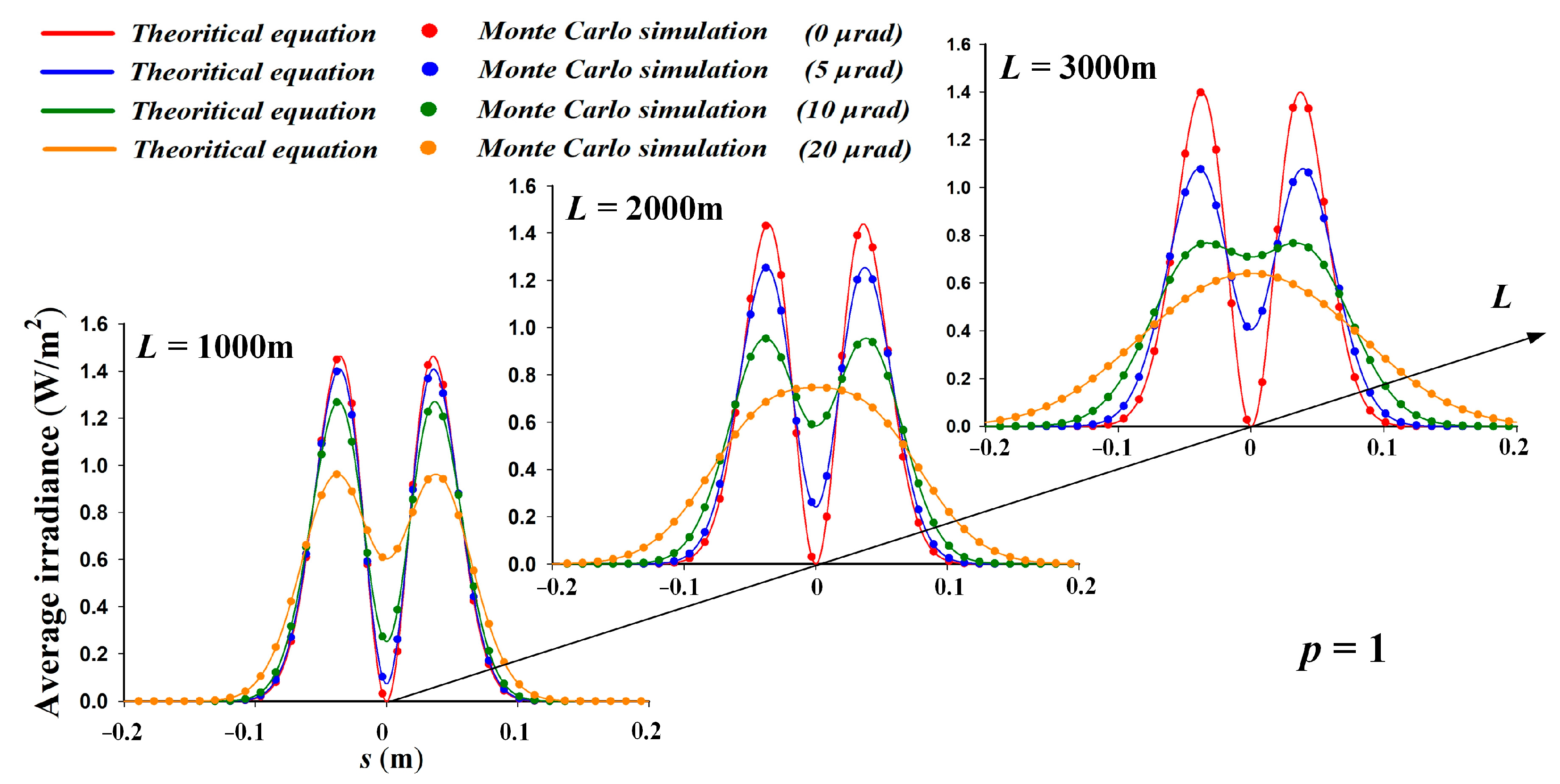
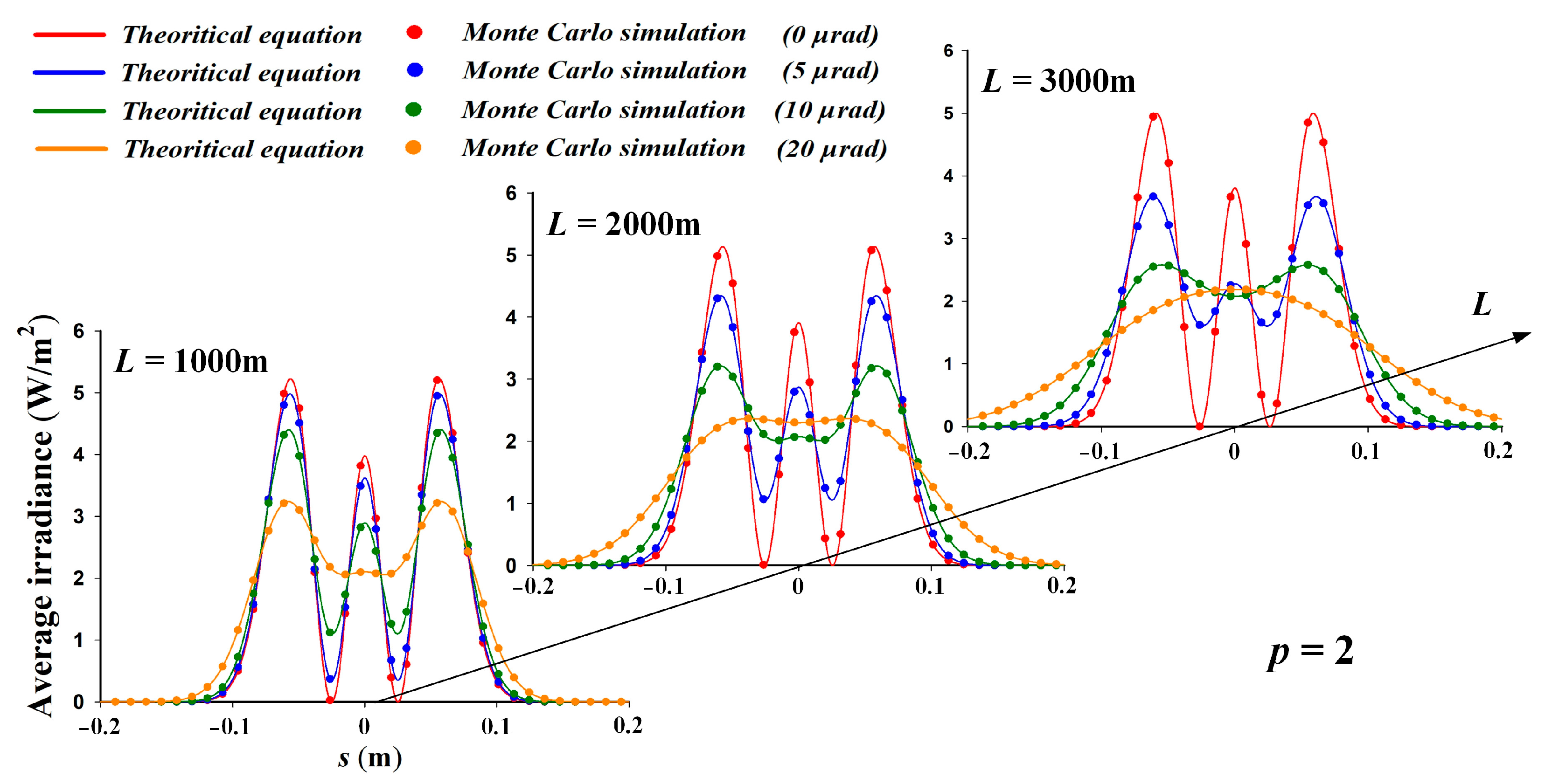
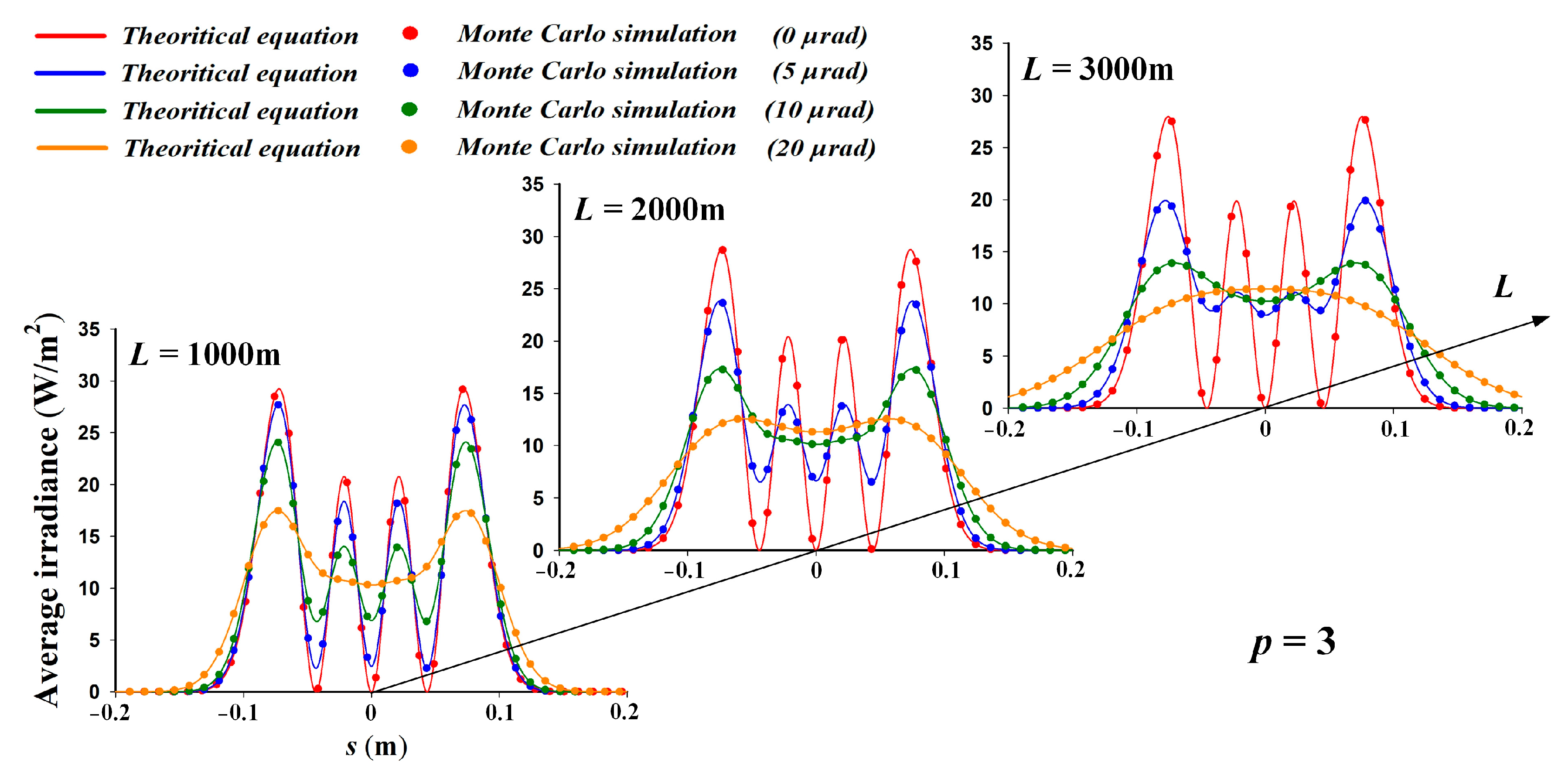
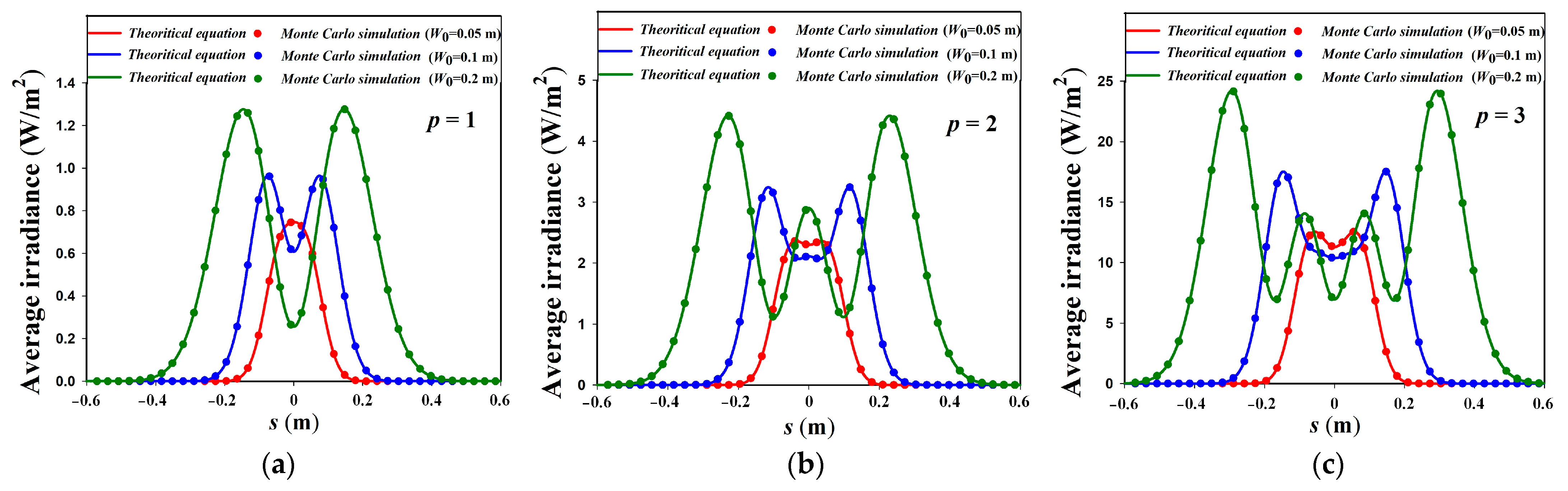
3. Numerical Simulation Results and Verification

The Monte Carlo simulation is widely used in FSOC system link simulation [19,20]. In this section, we adopted Monte Carlo simulation to design the propagation process of an HG beam under pointing error.

The random variation at the receiver caused by the pointing error can be generated using the Monte Carlo method. The detailed simulation process is shown as follows:

Combined with Equations (1)–(3), the instantaneous HG beam irradiance deviating under the influence of pointing error can be calculated as follows:

$$I_{mn}^p(x,y,L)=I_{mn}(x-r_x,y-r_y,L)$$

(7)

where $r_x$ and $r_y$ are generated by Equations (2) and (3), respectively.

Then, the simulated average irradiance under pointing error can be obtained statistically, which is shown as follows:

$${\langle I_{mn}(x,y,L)\rangle }^{\prime }{}_{PE}=\frac{1}{M}{\displaystyle \sum _{j=1}^M{I}_{mn}^p(x,y,L)}$$

(8)

where j denotes a serial number from 1 to M and $I_{mn}^p(x,y,L)$ denotes the j-th simulated speckle irradiance moving under the j-th simulated pointing error.

The numerical simulation parameters were set as follows: beam waist at transmitter W₀ = 0.05 m, wavelength λ = 850 nm and propagation distance L changes from 1000 to 3000 m. According to Equations (2) and (3), 10,000 groups of random displacements along the horizontal and vertical axes were generated, and the standard variance of the pointing error angle was set as 0, 5, 10 and 20 μrad. The simulation parameters are set in

Table 2. Simulation parameter settings.

Parameters	Value
Optical beam waist (W0)	0.05 m
Wavelength (λ)	850 nm
Propagation distance (L)	1000, 2000 and 3000 m
Standard variance of pointing error angle (${\sigma }_r$)	0, 5, 10 and 20 μrad
Grid points (N × N)	1024 × 1024
Simulated numbers (M)	10,000

; they are often used in practical FSOC systems.

For a satellite–satellite FSOC link, owing to the difference in the selection of tracking mechanism, the magnitudes of pointing error are equal to several microradians (μrad) to several tens of microradians (μrad) [4]. Especially for small satellite FSOC links, the fine pointing of small satellite FSOC links is primarily dependent on the fast-steering mirror (FSM) of microelectromechanical systems (MEMSs) with lower precision and smaller size, and the pointing error commonly reaches several tens of microradians (μrad) [21]. In this condition, the deduced average irradiance for the HG beam under arbitrary pointing error can provide guidance for theoretical analysis.

In Figure 2, Figure 3 and Figure 4, the lines represent the theoretical equations in Table 1, and the dots represent the results of the Monte Carlo simulation. Red, blue, green and yellow represent the results of the standard variance of the pointing error angle equal to 0, 5, 10, and 20 μrad, respectively. The correlation coefficients between the theoretical and simulation results were all greater than 0.999, which proves that the simulation results coincide with the deduced closed-form expressions. Notably, the numerical results of the proposed model are the same as Kiasaleh’s results under a small pointing error, and we provide the results of a large pointing error.

In the absence of the pointing error, the HG beam irradiance distribution is well preserved with an increase in the propagation distance when p = 1, 2,and 3. With the increase in pointing error and propagation distance, the valleys of the HG beam profile rise and converge toward the central origin, the profile changes into concave shape and then from concave shape to an approximately flat-top shape and, finally, the profile changes into an approximately Gaussian shape. This variation of the average irradiance profile with the increase in pointing error and propagation distance was first discovered. Additionally, the profile variation of a higher-order HG beam is slower than that of a lower-order HG beam under the same propagation conditions.

The average irradiance of the HG beam under the pointing error with different beam waists at the transmitter is illustrated in Figure 5. The beam waist at the transmitter was set as 0.05, 0.1 and 0.2 m. The standard variance of the pointing error was 20 μrad, and the propagation distance L = 2000 m. The other parameters were the same as those described initially. The lines represent the theoretical equations listed in Table 1, and the dots represent the results of the Monte Carlo simulation. Red, blue and green represent the beam waists at transmitter W₀ = 0.05, 0.1, and 0.2 m, respectively. Figure 5a–c shows the cases of p = 1, 2 and 3, respectively. We found that a larger beam waist at the transmitter could mitigate the profile change of the average irradiance of the HG beam under an increasing pointing error. Therefore, the original profile of the HG beam can be maintained by properly increasing the beam waist and controlling the standard variance of pointing error.

4. Discussion

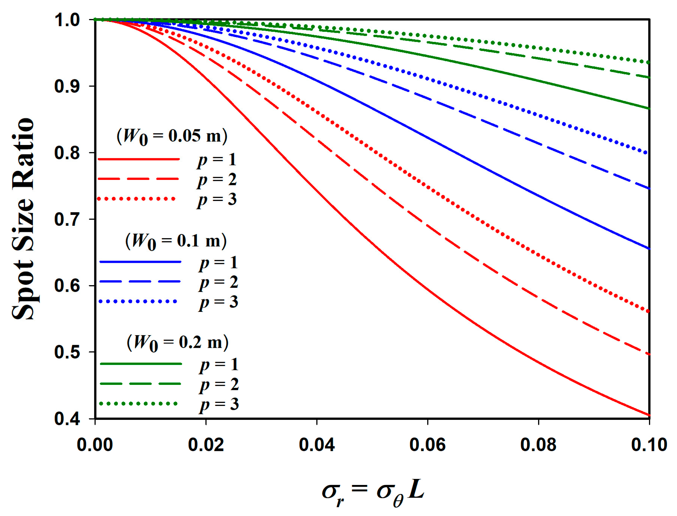
4.1. Effective Spot Size

Different from the lowest-order TEM₀₀ Gaussian beam, the HG beam forms a pattern of spots rather than a single spot of light; the conventional spot size W of a Gaussian beam is not suitable for an HG beam, and a new definition of the spot size of an HG beam is needed.

Carter et al. defined the “effective spot size” of an HG beam without pointing error [5,7,11]:

$${\rho }_{s,p}(L)={\rho }_{x,m}(L)\times {\rho }_{y,n}(L).$$

(9)

The terms ${\rho }_{x,m}(L)$ and ${\rho }_{y,n}(L)$ represent the spot size of the p-th mode [5,7,11]:

$${\rho }_{s,p}^2(L)=\frac{4{\displaystyle {\int }_{-\infty }^{\infty }{\displaystyle {\int }_{-\infty }^{\infty }{s}^2{I}_{mn}(x,y,z)dxdy}}}{{\displaystyle {\int }_{-\infty }^{\infty }{\displaystyle {\int }_{-\infty }^{\infty }{I}_{mn}(x,y,z)dxdy}}},$$

(10)

where p represents either m or n, and s represents either x or y.

Based on Equations (1) and (10), ${\rho }_{x,m}(L)$ and ${\rho }_{y,n}(L)$ can be rewritten as follows [5,7]:

$${\rho }_{x,m}^2(L)=(2m+1)W^2,$$

(11)

$${\rho }_{y,n}^2(L)=(2n+1)W^2.$$

(12)

In the presence of a pointing error, substituting Equation (5) into Equation (10), the spot size under the pointing error can be deduced as follows:

$${\rho }_{x,m}^2{(L)}_{PE}=(2m+1)W^2+4{\sigma }_r^2,$$

(13)

$${\rho }_{y,n}^2{(L)}_{PE}=(2n+1)W^2+4{\sigma }_r^2.$$

(14)

Equations (13) and (14) show that the pointing error increases the spot size of the HG beam. The spot size ratio is defined as ${\rho }_{s,p}^2(L)/{\rho }_{s,p}^2{(L)}_{PE}$, where p represents either m or n, s represents either x or y, and m can be replaced by n with the same result. In Figure 6, red, blue and green represent the beam waist at transmitter W₀ equal to 0.05, 0.1 and 0.2 m, respectively. We found that the effective spot size of the higher-order HG beam experiences less broadening under the pointing error than that of the lower-order HG beam. Meanwhile, the pointing error-induced HG beam spot size broadening decreased with an increase in the beam waist at the transmitter.

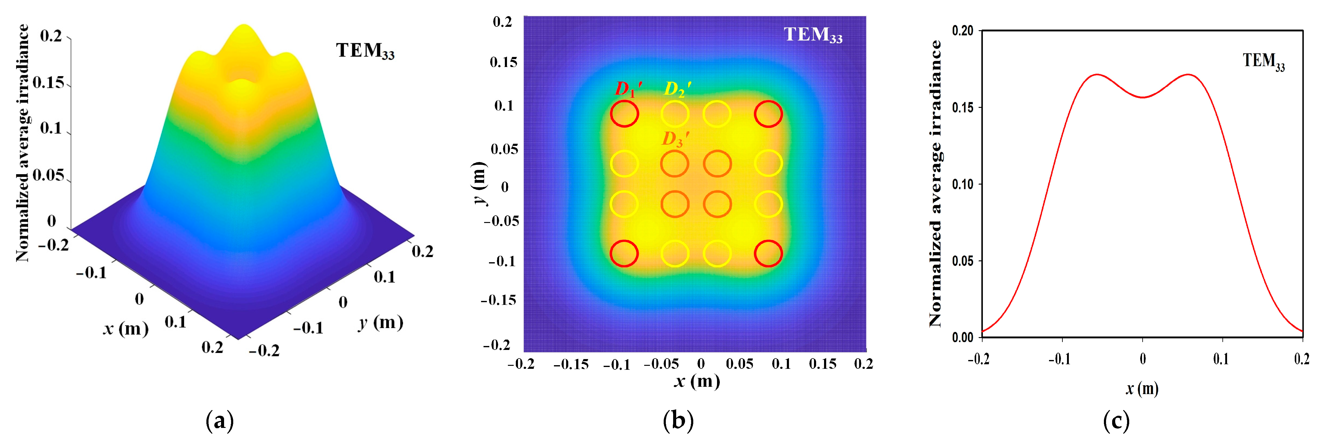
4.2. Location of the Local Extreme Value in the Average Irradiance under Pointing Error

The higher-order HG beam forms a pattern of spots rather than a single spot of an optical beam. Therefore, the location of each spot is necessary for the formulation of the receiving scheme.

According to the expressions in Table 1, the location of the local extreme value in the average irradiance under the pointing error can be obtained by solving the equation $d{\langle I_p(s,L)\rangle }_{PE}/ds=0$ and determining by the positive and negative of equation $d^2{\langle I_p(s,L)\rangle }_{PE}/d{s}^2$, where p represents either m or n, and s represents either x or y.

The locations of the local maxima and minima in the average irradiance under the pointing error are listed in

Table 3. Locations of local maxima and minima value in the average irradiance under pointing error.

Locations of the local maxima	p
$\pm \frac{\sqrt{W^4+2W^2{\sigma }_r^2-8{\sigma }_r^4}}{\sqrt{2}W}$; $\pm \frac{W}{\sqrt{2}}$ (${\sigma }_r=0$).	1
0, $\pm \sqrt{\frac{3W^2}{4}+{\sigma }_r^2-\frac{16{\sigma }_r^4-\sqrt{W^8+4W^6{\sigma }_r^2-8W^4{\sigma }_r^4+128{\sigma }_r^8}}{2W^2}}$; 0, $\pm \frac{\sqrt{5}W}{2}$ (${\sigma }_r=0$).	2
$\pm \sqrt{\frac{5W^{16}+16W^{14}{\sigma }_r^2-64W^{12}{\sigma }_r^4+4W^6{\sigma }_r^2{q}^{1/3}-48W^4{\sigma }_r^4{q}^{1/3}+q^{2/3}+4W^8(192{\sigma }_r^8+q^{1/3})}{4W^6{q}^{1/3}}}$, $\pm \sqrt{\frac{\left[5W^{16}-16W^{14}{\sigma }_r^2+64W^{12}{\sigma }_r^4+8W^6{\sigma }_r^2\right]q^{1/3}-96W^4{\sigma }_r^4{q}^{1/3}-q^{2/3}+8W^8\left[96{\sigma }_r^8+q^{1/3}\right]}{8W^6{q}^{1/3}}}$; $\pm \frac{\sqrt{3}W}{2}$, $\pm \frac{\sqrt{9W^2+\sqrt{57}{W}^2}}{2\sqrt{2}}$ (${\sigma }_r=0$).	3
Locations of the local minima	p
0	1
$\pm \sqrt{\frac{3W^2}{4}+{\sigma }_r^2-\frac{16{\sigma }_r^4+\sqrt{W^8+4W^6{\sigma }_r^2-8W^4{\sigma }_r^4+128{\sigma }_r^8}}{2W^2}}$; $\pm \frac{W}{2}$ (${\sigma }_r=0$).	2
0,$\pm \sqrt{\frac{\left[-5W^{16}-16W^{14}{\sigma }_r^2+64W^{12}{\sigma }_r^4+8W^6{\sigma }_r^2\right]q^{1/3}-96W^4{\sigma }_r^4{q}^{1/3}-q^{2/3}-8W^8\left[96{\sigma }_r^8+q^{1/3}\right]}{8W^6{q}^{1/3}}}$; 0, $\pm \frac{\sqrt{9W^2-\sqrt{57}{W}^2}}{2\sqrt{2}}$ (${\sigma }_r=0$).	3

.

The term q in Table 3 represents an expression associated with W and ${\sigma }_r$ and is obtained as follows:

$$\begin{array}{cc}\hfill q& =\left[W^{12}{(W^2+4{\sigma }_r^2)}^3\right](7W^6-36W^4{\sigma }_r^2+144W^2{\sigma }_r^4-192{\sigma }_r^6)+2\sqrt{-W^{24}{(W^2+4{\sigma }_r^2)}^6}\hfill \\ & \times \sqrt{(19W^{12}-324W^{10}{\sigma }_r^2+2232W^8{\sigma }_r^4-8832W^6{\sigma }_r^6+20736W^4{\sigma }_r^8-27648W^2{\sigma }_r^{10}+18432{\sigma }_r^{12})}\hfill \end{array}$$

(15)

Because m and n represent the order in the x and y axes, the coordinates of local extreme value locations can be determined by the location along the x and y axes. Taking ${\langle I_{21}(x,y,L)\rangle }_{PE}$ for instance, the locations of local maxima and local minima of irradiance are shown in

Table 4. Locations of local maxima and minima for TEM₂₁ Hermite–Gaussian beam.

In the presence of pointing error
$\left(0,-\frac{\sqrt{W^4+2W^2{\sigma }_r^2-8{\sigma }_r^4}}{\sqrt{2}W}\right)$, $\left(0,\frac{\sqrt{W^4+2W^2{\sigma }_r^2-8{\sigma }_r^4}}{\sqrt{2}W}\right)$, $\left(-\sqrt{\frac{3W^2}{4}+{\sigma }_r^2-\frac{16{\sigma }_r^4-\sqrt{W^8+4W^6{\sigma }_r^2-8W^4{\sigma }_r^4+128{\sigma }_r^8}}{2W^2}}, -\frac{\sqrt{W^4+2W^2{\sigma }_r^2-8{\sigma }_r^4}}{\sqrt{2}W}\right)$, $\left(\sqrt{\frac{3W^2}{4}+{\sigma }_r^2-\frac{16{\sigma }_r^4-\sqrt{W^8+4W^6{\sigma }_r^2-8W^4{\sigma }_r^4+128{\sigma }_r^8}}{2W^2}}, -\frac{\sqrt{W^4+2W^2{\sigma }_r^2-8{\sigma }_r^4}}{\sqrt{2}W}\right)$, $\left(-\sqrt{\frac{3W^2}{4}+{\sigma }_r^2-\frac{16{\sigma }_r^4-\sqrt{W^8+4W^6{\sigma }_r^2-8W^4{\sigma }_r^4+128{\sigma }_r^8}}{2W^2}}, \frac{\sqrt{W^4+2W^2{\sigma }_r^2-8{\sigma }_r^4}}{\sqrt{2}W}\right)$, $\left(\sqrt{\frac{3W^2}{4}+{\sigma }_r^2-\frac{16{\sigma }_r^4-\sqrt{W^8+4W^6{\sigma }_r^2-8W^4{\sigma }_r^4+128{\sigma }_r^8}}{2W^2}}, \frac{\sqrt{W^4+2W^2{\sigma }_r^2-8{\sigma }_r^4}}{\sqrt{2}W}\right)$.	Coordinates of the local maximum irradiance
$\left(x,0\right)$, $\left(-\sqrt{\frac{3W^2}{4}+{\sigma }_r^2-\frac{16{\sigma }_r^4+\sqrt{W^8+4W^6{\sigma }_r^2-8W^4{\sigma }_r^4+128{\sigma }_r^8}}{2W^2}},y\right)$, $\left(\sqrt{\frac{3W^2}{4}+{\sigma }_r^2-\frac{16{\sigma }_r^4+\sqrt{W^8+4W^6{\sigma }_r^2-8W^4{\sigma }_r^4+128{\sigma }_r^8}}{2W^2}},y\right)$.	Coordinates of the local minimum irradiance
In the absence of pointing error
$\left(-\frac{\sqrt{5}W}{2},-\frac{W}{\sqrt{2}}\right)$, $\left(0,-\frac{W}{\sqrt{2}}\right)$, $\left(\frac{\sqrt{5}W}{2},-\frac{W}{\sqrt{2}}\right)$, $\left(-\frac{\sqrt{5}W}{2},\frac{W}{\sqrt{2}}\right)$, $\left(0,\frac{W}{\sqrt{2}}\right)$, $\left(\frac{\sqrt{5}W}{2},\frac{W}{\sqrt{2}}\right)$.	Coordinates of the local maximum irradiance
$\left(x,0\right)$, $\left(-\frac{W}{2},y\right)$, $\left(\frac{W}{2},y\right)$.	Coordinates of the local minimum irradiance

.

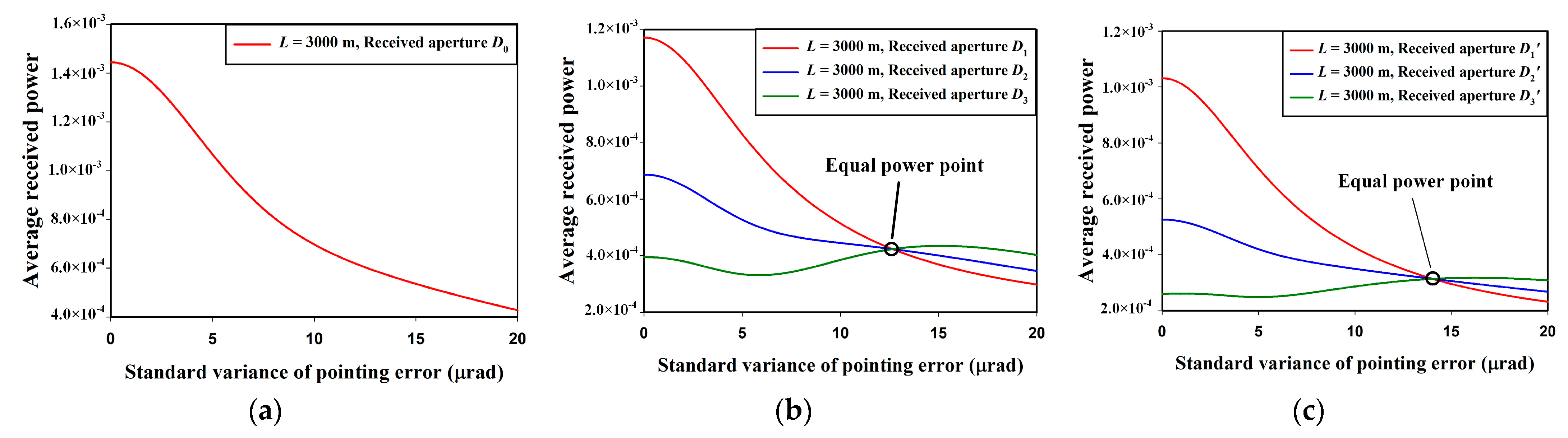
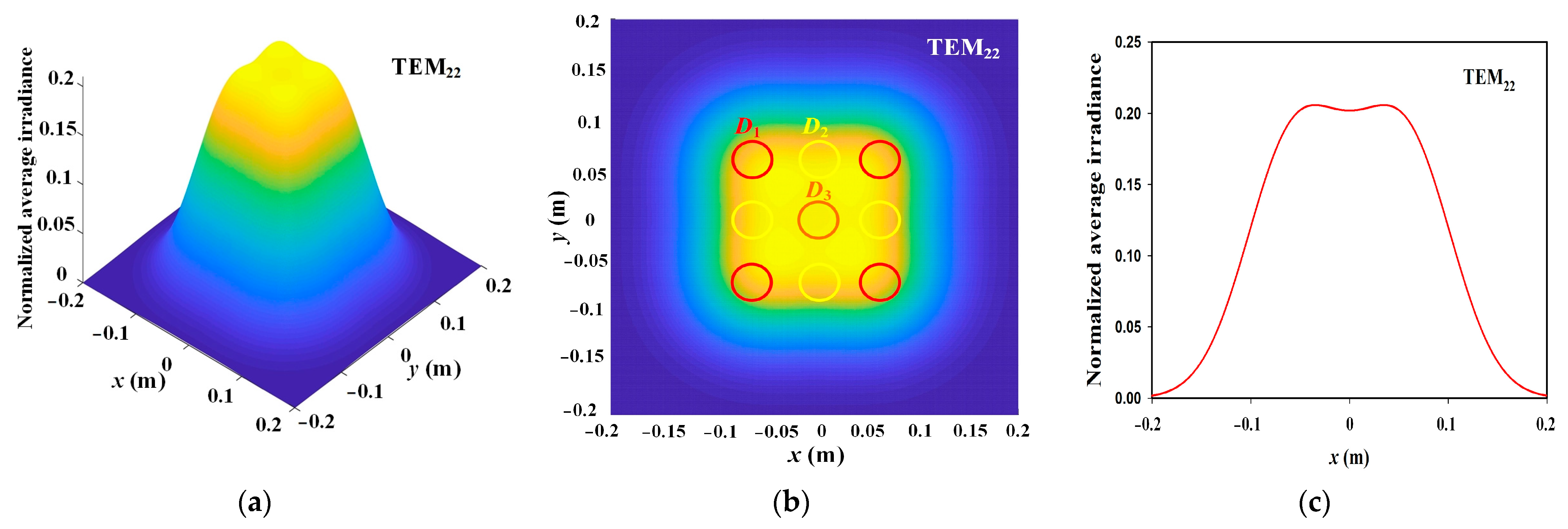
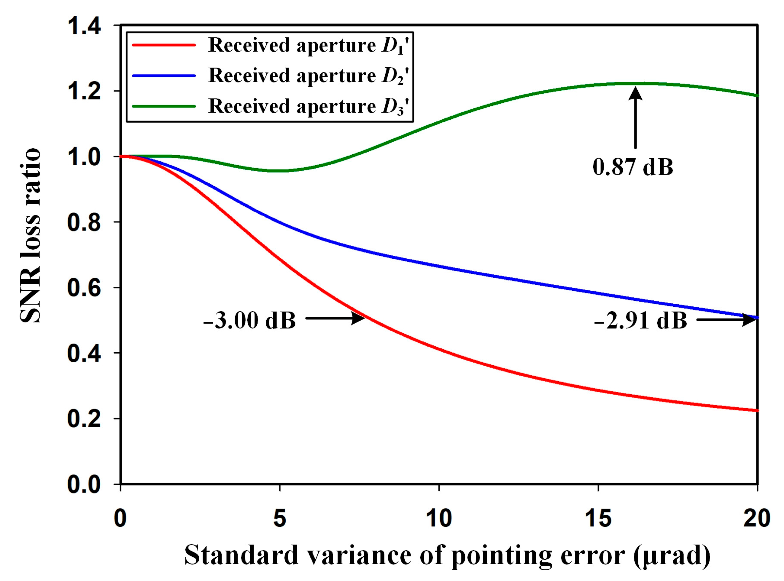
4.3. Average Received Power and SNR Loss

Based on the aforementioned research on the average irradiance of the HG beam under the pointing error and location of the local maxima, the average received power at the location of the local maxima can be further deduced for the HG-based FSOC with (SIMO).

As shown in Figure 7, the three common modes of the HG beam, TEM₁₁, TEM₂₂ and TEM₃₃, are selected for the average received power investigation. Each array receiving the aperture center is located at the location of the local maxima. The TEM₁₁ HG beam irradiance without pointing error had four local maximum points, and their peak irradiances were equal. Therefore, the receiving aperture D₀ is arranged at four locations of the local maxima. The TEM₂₂ HG beam without pointing error has nine local maximum points, which can be divided into three groups according to their peak irradiance. Therefore, the receiving apertures D₁, D₂ and D₃ were arranged at nine locations of the local maxima (see Figure 7b). Similarly, the TEM₃₃ HG beam without pointing error has 16 local maxima points, and it can also be divided into three groups according to their peak irradiance: the receiving apertures D₁’, D₂’ and D₃’ are arranged at 16 locations of local maxima (see Figure 7c). Taking the TEM₃₃ HG beam as an example, the receiving apertures are the same but are divided into three groups according to the peak irradiance (red, yellow and orange), and the average received power values of similar color receiving apertures are equal.

The average received power under the pointing error can be formulated by integrating the average irradiance under the pointing error of the receiving aperture. Based on Equation (5), the average received power for the HG beam under the pointing error is formulated as follows:

$$P(D)={\displaystyle \underset{D}{\iint }{\langle I_{mn}(x,y,L)\rangle }_{PE}}dxdy$$

(16)

where D denotes the diameter of the circular receiving aperture. However, Equation (16) cannot be integrated over a circular area when the receiving aperture is not located at the center of the main propagation axis. Inspired by [21,22], we use a square within the same area to substitute the circle as the integration area. The square length l is equal to $0.5\sqrt{\pi }D$. Assuming that the coordinates of the center of the receiving aperture are (x_f, y_f), Equation (16) can be approximated as follows:

$$P(D)\approx {\displaystyle {\int }_{x_f-l}^{x_f+l}{\displaystyle {\int }_{y_f-l}^{y_f+l}{\langle I_{mn}(x,y,L)\rangle }_{PE}}}dxdy$$

(17)

When taking the values of m and n, the expressions for the average received power corresponding to TEM₁₁, TEM₂₂ and TEM₃₃ are as follows:

$$\begin{array}{cc}\hfill P_{11}& =\frac{W_0^2}{4W_E^{10}}\{\exp \left(-T_{11}^2-T_{21}^2\right)\left[\sqrt{2\pi }{W}_E^{3}erf(T_{11})\exp (T_{11}^2)-4(l+x_f)W^2\right]\hfill \\ & -\exp \left(-T_{12}^2-T_{21}^2\right)\left[\sqrt{2\pi }{W}_E^{3}erf(-T_{12})\exp (T_{12}^2)+4(l-x_f)W^2\right]\}\hfill \\ & \times \left\{4W^2\left[\exp (T_{21}^2)(y_f-l)-\exp (T_{22}^2)(l+y_f)\right]+\sqrt{2\pi }{W}_E^3\exp (T_{21}^2)\left[erf(T_{21})+erf(T_{22})\right]\right\}\hfill \end{array},$$

(18)

$$\begin{array}{cc}\hfill P_{22}& =\frac{4W_0^2}{W_E^{18}}\{\left[\sqrt{2\pi }{W}_E^7\exp (T_{11}^2)erf(T_{11})-2(l+x_f)W^2(W^4+4W^2{(l+x_f)}^2+5{\sigma }_r^2+64{\sigma }_r^4)\right]\hfill \\ & \times \exp \left(-T_{11}^2-T_{21}^2\right)-[\sqrt{2\pi }{W}_E^7\exp (T_{12}^2)erf(-T_{12})+2(l-x_f)W^2(W^4+4W^2{(l-x_f)}^2\hfill \\ & +5{\sigma }_r^2+64{\sigma }_r^4)]\exp \left(-T_{12}^2-T_{21}^2\right)\}\times \{\sqrt{2\pi }{W}_E^7\exp (T_{21}^2)\left[erf(T_{21})+erf(T_{22})\right]\hfill \\ & -2W^2[\left(1+\exp (T_3)\right)\left(12l^2{y}_f{W}^2+4l^3{W}^2+20l{W}^2{\sigma }_r^2+64l{\sigma }_r^4\right)\hfill \\ & +\left(1-\exp (T_3)\right)\left(4l^3{W}^2+12l{y}_f^2{W}^2+l{W}^4+20l{W}^2{\sigma }_r^2+64l{\sigma }_r^4\right)]\}\hfill \end{array},$$

(19)

$$\begin{array}{cc}\hfill P_{33}& =\frac{16W_0^2}{W_E^{26}}\{3\sqrt{2\pi }{W}_E^{11}erf(-T_{12})-3\sqrt{2\pi }{W}_E^{11}erf(T_{11})+4\exp (-T_{11}^2)(l+x_f)\hfill \\ & \times W^2[3W^8+2304{\sigma }_r^8-2W^6\left({(l+x_f)}^2-21{\sigma }_r^2\right)+288W^2{\sigma }_r^4\left({(l+x_f)}^2+5{\sigma }_r^2\right)\hfill \\ & +8W^4\left({(l+x_f)}^4+8{(l+x_f)}^2{\sigma }_r^2-42{\sigma }_r^4\right)]+4\exp (-T_{12}^2)(l-x_f)W^2\hfill \\ & \times [3W^8+2304{\sigma }_r^8-2W^6\left({(l+x_f)}^2-21{\sigma }_r^2\right)+288W^2{\sigma }_r^4\left({(l+x_f)}^2+5{\sigma }_r^2\right)\hfill \\ & +8W^4\left({(l+x_f)}^4+8{(l+x_f)}^2{\sigma }_r^2-42{\sigma }_r^4\right)]\}\{4W^2\{\left[\exp (T_{21}^2)+\exp (T_{22}^2)\right]\hfill \\ & \times [l\left[40l^4{W}^4+3W_E^4(W^4+6W^2{\sigma }_r^2+48{\sigma }_r^4)-6l^2(W^6-32W^4{\sigma }_r^2-144W^2{\sigma }_r^4)\right]+8l^5{W}^4\hfill \\ & +2l^3{W}^2(40y_f^2{W}^2-W^4+32W^2{\sigma }_r^2+144{\sigma }_r^4)]-3\sqrt{2\pi }{W}_E^{11}erf(T_4)-3\sqrt{2\pi }{W}_E^{11}erf(T_4)\hfill \\ & +\left[\exp (T_{22}^2)-\exp (T_{21}^2)\right][40l^4{y}_f{W}^4+2l^2{y}_f{W}^2(40l^2{W}^2-3W^4+96W^2{\sigma }_r^2+432{\sigma }_r^4)\hfill \\ & +l\left[8y_f^4{W}^4+3W_E^4(W^4+6W^2{\sigma }_r^2)+48{\sigma }_r^4+l^2(-2W^6+64W^4{\sigma }_r^2+288W^2{\sigma }_r^4)\right]\}\}\hfill \end{array},$$

(20)

where $W_E^2=W^2+4{\sigma }_r^2$, $T_{11}\frac{\sqrt{2}(l+x_f)}{W_E}$, $T_{12}\frac{\sqrt{2}(l-x_f)}{W_E}$, $T_{21}\frac{\sqrt{2}(l+y_f)}{W_E}$, $T_{22}\frac{\sqrt{2}(l-y_f)}{W_E}$, $T_3=\frac{8y_{f}l}{W_E^2}$, $T_4=\frac{4(y_f^2+l^2)}{W_E^2}$ and $erf\left(\right)$ is an error function.

As shown in Figure 8a, for the TEM₁₁ HG beam, the average received power on the receiving aperture D₀ decreases with an increase in the pointing error. As shown in Figure 8b, for the TEM₂₂ HG beam, the average received power on D₁ and D₂ decreased with an increase in the pointing error, and the average received power on D₁ decreased faster than the average received power on D₂. The average received power on D₃ fluctuated with an increase in the pointing error. Notably, the average received powers on D₁, D₂ and D₃ are equal when ${\sigma }_r$ = 12.67 μrad; we define it as the “equal power point”. As shown in Figure 8c, for the TEM₃₃ HG beam, the variation trend of the average received power on D₁’, D₂’ and D₃’ with an increase in the pointing error was the same as that of the TEM₂₂ HG beam. The “equal power point” appears at ${\sigma }_r$ = 14.05 μrad.

As shown in Figure 9, the average irradiance of the TEM₂₂ HG beam at the “equal power point” ${\sigma }_r$ = 12.67 μrad exhibits a flat-topped profile. As shown in Figure 10, the average irradiance of the TEM₃₃ HG beam at the “equal power point” ${\sigma }_r$ = 14.05 μrad exhibits a slightly hollow shape. The average irradiance of the HG beam appears to have a nearly flat-topped shape at the “equal power point”.

The TEM₃₃ HG beam is taken as an example to analyze the received power loss ratio (also SNR loss ratio) under the influence of pointing error in the corresponding receiving aperture. The numerical simulation parameters are the same as above, and the transmission distance is 3000 m.

As shown in Figure 11, with the increase in pointing error, the loss of average SNR is 3.00 dB when ${\sigma }_r$ = 7.89 μrad at receiving aperture D1’, the loss of average SNR is 2.91 dB when ${\sigma }_r$ = 20 μrad at receiving aperture D₂’ and the average SNR decaying speed of receiving aperture D₁’ is faster than that of receiving aperture D₂’. For receiving aperture D₃’, the average SNR decreases and then increases with the increase in pointing error, and the increase in average SNR is 0.87 dB when ${\sigma }_r$ = 16.97 μrad. This shows that the transmitted power is homogenized at the receiver under the influence of pointing error. In order to achieve better reception efficiency for the HG beam, we should control the transmission parameters. It can be seen that when the propagation parameter is set as shown in Table 2, the standard variance of pointing error should be less than 7.5 μrad for the TEM₃₃ HG beam so that the SNR loss at each receiving aperture is less than 3.00 dB.

5. Conclusions

The closed-form expression of the average irradiance of the HG beam under the pointing error was deduced through a statistical averaging method and verified by Monte Carlo simulation. The correlation coefficient between deduced theoretical expression and Monte Carlo simulation reaches 0.999. We firstly found that the valleys of the HG beam profile rise and converge toward the central origin, the profile changes into a concave shape and then from a concave shape to an approximately flat-top shape and, finally, the profile changes into an approximately Gaussian shape, and the larger beam waist at the transmitter could mitigate the profile change of the average irradiance of the HG beam under increasing pointing error. The effective spot size, location of the local extreme value and average received power for the average irradiance under the pointing error were theoretically deduced for the first time. The spot size will be broadened under the influence of the pointing error, the location of the local extreme value will change with the variation of the pointing error and the average received power at the local extreme value fluctuates under different pointing errors. Moreover, the pointing error causes SNR loss in the receiving aperture that has been analyzed. For the TEM₃₃ HG beam, the standard variance of pointing error should be within 7.5 μrad so that the SNR loss at each receiving aperture is less than 3.00 dB with the transmission distance of 3000 m. The fundamental theoretical expressions of average irradiance for an HG beam under pointing error have provided effective guidance for analyzing the propagation characteristics and link performance.

Further research on the average irradiance for an HG beam under pointing error in atmospheric turbulence should be conducted. Under the influence of atmospheric turbulence, the optical field is disturbed and more random processes are introduced. Further research may prove theoretical guidance for HG beams used in atmospheric turbulence. The average bit error rate and fade probability for an HG beam-based FSOC link should also be studied in following work.

References

1. You, X.; Wang, C.; Huang, J.; Gao, X.; Zhang, Z.; Wang, M.; Huang, Y.; Zhang, C.; Jiang, Y.; Wang, J.; et al. Towards 6G wireless communication networks: Vision, enabling technologies, and new paradigm shifts. Sci. China Inf. Sci. 2021, 64, 110301. [Google Scholar] [CrossRef]
2. Mansour, A.; Mesleh, R.; Abaza, M. New challenges in wireless and free space optical communications. Opt. Lasers Eng. 2017, 89, 95–108. [Google Scholar] [CrossRef]
3. Chowdhury, M.Z.; Hossan, M.T.; Islam, A.; Jang, Y.M. A Comparative Survey of Optical Wireless Technologies: Architectures and Applications. IEEE Access 2018, 6, 9819–9840. [Google Scholar] [CrossRef]
4. Kaushal, H.; Kaddoum, G. Optical Communication in Space: Challenges and Mitigation Techniques. IEEE Commun. Surv. Tutor. 2017, 19, 57–96. [Google Scholar] [CrossRef] [Green Version]
5. Andrews, L.C.; Phillips, R.L. Laser Beam Propagation through Random Media, 2nd ed.; SPIE: Bellingham, WA, USA, 2005. [Google Scholar]
6. Laabs, H. Propagation of Hermite-Gaussian-beams beyond the paraxial approximation. Opt. Commun. 1998, 147, 1–4. [Google Scholar] [CrossRef]
7. Young, C.Y.; Gilchrest, Y.V.; Macon, B.R. Turbulence induced beam spreading of higher order mode optical waves. Opt. Eng. 2002, 41, 1097–1103. [Google Scholar]
8. Kiasaleh, K. Statistical Profile of Hermite-Gaussian Beam in the Presence of Residual Spatial Jitter in FSO Communications. IEEE Commun. Lett. 2016, 20, 656–659. [Google Scholar] [CrossRef]
9. Kiasaleh, K. Spatial beam tracking for Hermite-Gaussian-based free-space optical communications. Opt. Eng. 2017, 56, 076106. [Google Scholar] [CrossRef]
10. Kiasaleh, K. Probability density function of Hermite-Gaussian beam intensity in the presence of spatial error. Opt. Eng. 2016, 55, 095109. [Google Scholar] [CrossRef]
11. Carter, W.H. Spot size and divergence for Hermite Gaussian beams of any order. Appl. Opt. 1980, 19, 1027–1029. [Google Scholar] [CrossRef] [PubMed]
12. Singh, M.; Chebaane, S.; Ben Khalifa, S.; Grover, A.; Dewra, S.; Angurala, M. Performance Evaluation of a 4 × 20-Gbps OFDM-Based FSO Link Incorporating Hybrid W-MDM Techniques. Front. Phys. 2021, 9, 746779. [Google Scholar] [CrossRef]
13. Chaudhary, S.; Lin, B.; Tang, X.; Wei, X.; Zhou, Z.; Lin, C.; Zhang, M.; Zhang, H. 40 Gbps-80 GHz PSK-MDM based Ro-FSO transmission system. Opt. Quantum Electron. 2018, 50, 321. [Google Scholar] [CrossRef]
14. Boobalan, S.; Prakash, S.A.; Angurala, M.; Malhotra, J.; Singh, M. Performance Enhancement of 3 × 20 Gbit/s MDM-Based OFDM-FSO System. Wirel. Pers. Commun. 2022, 122, 3137–3165. [Google Scholar] [CrossRef]
15. Pang, K.; Song, H.; Zhao, Z.; Zhang, R.; Song, H.; Xie, G.; Li, L.; Liu, C.; Du, J.; Molisch, A.F.; et al. 400-Gbit/s QPSK free-space optical communication link based on four-fold multiplexing of Hermite-Gaussian or Laguerre-Gaussian modes by varying both modal indices. Opt. Lett. 2018, 43, 3889–3892. [Google Scholar] [CrossRef] [PubMed]
16. Kaymak, Y.; Rojas-Cessa, R.; Feng, J.; Ansari, N.; Zhou, M.; Zhang, T. A Survey on Acquisition, Tracking, and Pointing Mechanisms for Mobile Free-Space Optical Communications. IEEE Commun. Surv. Tutor. 2018, 20, 1104–1123. [Google Scholar] [CrossRef]
17. Kaushal, H.; Jain, V.K.; Kar, S. Free Space Optical Communication; Springer: New Delhi, India, 2017. [Google Scholar]
18. Magidi, S.; Jabeena, A. Free Space Optics, Channel Models and Hybrid Modulation Schemes: A Review. Wirel. Pers. Commun. 2021, 119, 2951–2974. [Google Scholar] [CrossRef]
19. Liu, X.; Jiang, D.; Hu, Z.; Zeng, Q.; Qin, K. Single-Layer Phase Screen with Pointing Errors for Free Space Optical Communication. IEEE Access 2021, 9, 104070–104078. [Google Scholar] [CrossRef]
20. Hu, S.; Liu, H.; Zhao, L.; Bian, X. The Link Attenuation Model Based on Monte Carlo Simulation for Laser Transmission in Fog Channel. IEEE Photonics J. 2020, 12, 1–10. [Google Scholar] [CrossRef]
21. Hu, Z.; Jiang, D.; Liu, X.; Zhu, B.; Zeng, Q.; Qin, K. Performance research on flat-topped beam-based small satellites free space optical communication. Opt. Commun. 2021, 487, 126802. [Google Scholar] [CrossRef]
22. Bashir, M.; Alouini, M. Optimal Power Allocation Between Beam Tracking and Symbol Detection Channels in a Free-Space Optical Communications Receiver. IEEE Trans. Commun. 2021, 69, 7631–7646. [Google Scholar] [CrossRef]
Figure 1. Forming process of average irradiance of HG beam under pointing error. (a) Propagation axis without pointing error, (b) Pointing error induced random deviation at different times, (c) Average irradiance under pointing error.
Photonics 09 00478 g001
Figure 2. Average irradiance of HG beam under pointing error with the increase in propagation distance in the case of p = 1.
Photonics 09 00478 g002
Figure 3. Average irradiance of HG beam under pointing error with the increase in propagation distance in the case of p = 2.
Photonics 09 00478 g003
Figure 4. Average irradiance of HG beam under pointing error with the increase in propagation distance in the case of p = 3.
Photonics 09 00478 g004
Figure 5. Average irradiance of HG beam under pointing error with different beam waists at transmitter. (a) p = 1, (b) p = 2 and (c) p = 3.
Photonics 09 00478 g005
Figure 6. Changes in HG beam spot size ratio with the increase in pointing error.
Photonics 09 00478 g006
Figure 7. Array receiving for HG beam. (a) TEM11, (b) TEM22 and (c) TEM33.
Photonics 09 00478 g007
Figure 8. Average received power at the corresponding receiving aperture under the influence of pointing error. (a) TEM11, (b) TEM22 and (c) TEM33.
Photonics 09 00478 g008
Figure 9. Average irradiance of TEM22 HG beam when σ r = 12.67 μrad. (a) A 3D diagram, (b) a vertical diagram and (c) a cross-section along the x axis.
Photonics 09 00478 g009
Figure 10. Average irradiance of TEM33 HG beam when σ r = 14.05 μrad. (a) A 3D diagram, (b) a vertical diagram and (c) a cross-section along the x axis.
Photonics 09 00478 g010
Figure 11. SNR loss ratio with the increase in pointing error.
Photonics 09 00478 g011