Review

Leveraging AI in Photonics and Beyond

Department of Electronics and Photonics, Institute of High Performance Computing, Agency for Science, Technology and Research (A*STAR), Singapore 138632, Singapore
*
Author to whom correspondence should be addressed.
These authors contributed equally to this work.
Photonics 2022, 9(2), 75; https://doi.org/10.3390/photonics9020075
Submission received: 25 November 2021 / Revised: 31 December 2021 / Accepted: 11 January 2022 / Published: 28 January 2022
(This article belongs to the Special Issue The Interplay between Photonics and Machine Learning)

Abstract

:
Artificial intelligence (AI) techniques have been spreading in most scientific areas and have become a heated focus in photonics research in recent years. Forward modeling and inverse design using AI can achieve high efficiency and accuracy for photonics components. With AI-assisted electronic circuit design for photonics components, more advanced photonics applications have emerged. Photonics benefit a great deal from AI, and AI, in turn, benefits from photonics by carrying out AI algorithms, such as complicated deep neural networks using photonics components that use photons rather than electrons. Beyond the photonics domain, other related research areas or topics governed by Maxwell’s equations share remarkable similarities in using the help of AI. The studies in computational electromagnetics, the design of microwave devices, as well as their various applications greatly benefit from AI. This article reviews leveraging AI in photonics modeling, simulation, and inverse design; leveraging photonics computing for implementing AI algorithms; and leveraging AI beyond photonics topics, such as microwaves and quantum-related topics.

1. Introduction

Electromagnetics is a fundamental branch of physics that arises from the interaction of charged particles with ever-expanding technological applications and scientific discoveries [1,2,3,4,5]. It has enormous implications in our daily life from medical applications to mobile phones. The electromagnetic spectrum encapsulates wavelengths from thousands of kilometers down to a fraction of the size of an atomic nucleus. In a celestial manner, the behavior of electromagnetic waves corresponding to this entire spectrum can be succinctly described by the golden set of Maxwell equations. Table 1 summarizes the spectrum distribution from Radiofrequency (RF) to Optics and the corresponding typical applications/techniques. As given in the table, the wide spectrum of optics (where photonics are mainly located) from far-infrared to ultraviolet yields numerous photonics applications [6,7,8].
Unlike other domains, the physics within Maxwell equations is complete and self-consistent in nature. However, one must employ hard computing to numerically seek solutions to these equations, which is computationally expensive and laborious. The modeling complexity of hard computing methods scales directly with the domain size and the required precision—limiting full exploration of the parameter space. Thus, interruptions of the traditional Maxwell equation-based method with Artificial intelligence (AI) are vital to advance the state-of-art in the design and modeling of electromagnetic problems [20,21,22]. AI methods, such as machine learning (ML) techniques are proven methodologies for the capture, interpolation, and optimization of highly complex phenomena in many fields. They are widely used in image classification [23,24], image/video processing [17,25,26], natural language processing (NLP) [27,28], and robotics [29,30]. Thus, coupling AI techniques with traditional physics-based methods could potentially discover pseudo-random designs with performance excellence that is beyond physical intuitions. This entire cycle of design, modeling, and simulation carried by soft computing algorithms will accelerate execution speeds by two to three orders of magnitude. Importantly, the intrinsic nature of ML algorithms, which is data-driven, allows the incorporation of many of the uncertainties in material parameters, fabrication, and manufacturing. Therefore, when viewed as a whole, the methodology will reduce fabrication tape-outs and cycles and increase manufacturing yield. As illustrated in Table 1, all the applications/techniques listed from RF to optics can leverage AI. For example, within the optics domain, infrared with AI techniques can help to detect the human body [14], analyze material composition [15], and colorize NIR images [16]. For the fields beyond optics, the related applications leveraging AI will be further discussed in Section 4.
With the rapid development of AI in recent years, especially the deep learning methods, how to leverage AI for photonics has attracted significant interest from researchers worldwide. Figure 1 shows the research trend on AI and photonics since 1996. The number of the publication with topics including AI and photonics from web of science is searched by conditions: AI (topic) or deep learning (topic) or machine learning topic) and photonics (topic) from 1996 to 2021. It can be seen from Figure 1 that the publications have increased dramatically since 2005 from 5000 to almost 50,000, and it is expected that such an increasing trend could last for years. A network visualization is also shown in Figure 1 based on the highly-cited paper from 2021, searched by web of science and plotted using VOSviewer [31].
This article reviews the applications of ML methods in electromagnetics with a particular emphasis on photonics. Photonics covers a wide range of the electromagnetic spectrum from visible to mid-infrared wavelengths. This encapsulates vast applications that include data transport, telecommunication, quantum information technologies, biology, and chemical sensing. The rest of this review paper is organized as follows. Section 2 describes the applications of AI on photonics modeling, simulation, and inverse design. The recent studies on soft computing using ML and the inverse design for photonics using Generative adversarial network (GAN) are summarized. Section 3 reviews the studies on how photonics contribute to AI in terms of implementing advanced Neural Networks using photonics hardware for acceleration. In Section 4, we review the AI applications beyond photonics, including AI for computational electromagnetics (forward and inverse solvers), microwave device optimization and design, electromagnetic compatibility and interference (EMC/EMI), and quantum-computing-related topics.

2. AI for Photonics: Modeling and Simulation

As indicated by Figure 1, the publications of photonics related to AI/deep learning have been drastically increased recently. There are several articles [32,33,34] reviewing applications of AI techniques in photonics. [32,33] target applications of AI methods for general device modeling in photonics, while [34] targets application of AI methods in exclusively in integrated quantum photonics. Device modeling in photonics can be broadly divided into forward and inverse modeling.
In forward modeling, the input parameter space consists of device geometrical parameters, and the output parameter space comprises the performance vectors. AI methods typically utilizes discriminative neural networks. Discriminative neural networks model the definite mapping between the input and output variables via multilayer feedforward networks or CNNs. These have been successfully applied in forward modeling of the spectral response of plasmonic scatters [35], effective refractive indices of waveguides [36], electric field profiles of photonics systems [37,38], dielectric metasurfaces [39,40,41], dielectric metagratings [42], beam combiners [43], beam steering devices [39], and photonics topological insulators [44]. On the other hand, in inverse modeling, as the name suggests, the inputs are the performance vectors, and the outputs are the corresponding device geometry. The AI methods in inverse modeling can be further categorized into three categories. The first category uses gradient descent-based algorithms coupled with a forward model. Here, the gradients of the forward model are evaluated either by adjoint methods [45,46] or automatic differentiation [40,47]. Automatic differentiation employs chain rules of derivatives, and they are mathematically equivalent to backpropagation algorithms. Starting from an educated guess of the device geometry, the error between the guess geometry response, and the desired response is calculated. This error is backpropagated, and a modified geometry is obtained. The process is repeated until the error between the guess and desired response is an acceptably small value. The second class of inverse methods makes use of conventional optimization techniques, such as genetic and particle swam algorithms and forward models. In this class, the optimization algorithm will conduct an algorithmic search for the device geometry with the desired performance, and the algorithms will access the forward model multiple times (depending on the problem the counts could be hundreds or thousands). The third class of inverse algorithm makes use of generative neural networks to predict the device geometry with desired performance targets [48,49,50], and the detail review will be given in Section 2.3. As explained above, the application of AI techniques in photonics thus far is vastly concentrated on device designs. Readers can refer to [32,33,34] for more details. In the following sections, we will take two specific areas for details discussions. The first is application of AI methods in for optical mode solving—a forward modeling problem, and the second is the application of generative neural networks in the inverse designs. Before we move to the AI applications in photonics, a brief introduction on some fundamentals of Neural Networks will be given in Section 2.1.

2.1. Neural Networks

Artificial Neural Network (ANN), Convolution Neural Network (CNN) and Recurrent Neural Network (RNN) are three most commonly used Neural Networks. ANN usually consists of three layers—input, hidden and output layers, connected in the forward direction. Each node of the input and hidden layers has parameters of weight and bias for the node connected to the next layer. ANN is capable of learning complex nonlinear function that maps any input to the desired output. For example, ref. [51] predicted hourly global, diffuse, and direct solar irradiance using ANN based on various measured data. However, ANN is only applicable when the input data size (the number of the nodes of the input layer) and the number of the nodes of the hidden layer are relatively small because the number of trainable parameters (weights and bias) increases drastically as the numbers of input layer nodes and the hidden layers increase. In addition, ANN loses the spatial/temporal features of the input data, such as images and video, and it cannot capture sequential information in the input data, such as time series data. CNN is prevalent in the deep learning community, especially in computer vision. Unlike ANN, the trainable parameters lie in the filters, also called kernels. Instead of fully connecting all the nodes in each layers, the filters are used to extract the relevant features from the input using the convolution operation. For instance, ref. [52] used CNN to extract high-level features of computed tomography data to diagnose COVID-19 symptoms. RNN is widely used in natural language processing with sequential input data. It has a recurrent connection on the hidden layers and shares parameters across different time steps. This results in fewer parameters to train and decreases the computational cost. In [38], a RNN is employed to establish the field continuity between the adjacent pixels for the calculation of optical mode profiles. Based on the three essential NNs, many machine learning frameworks/models, such as ResNet [23], GAN [53,54], LSTM [55,56], and Transformer [57] have been built for solving various complicated problems.

2.2. Optical Mode Solving

Traditionally the design tasks in photonics are carried out using physical principles and intuitions. However, this does not explore the full input parameter space constrained by the available materials and fabrication techniques. The modeling and simulation in photonics are governed by the golden set of Maxwell equations. The physics within Maxwell equations is complete and self-consistent in nature. However, one must employ hard computing to numerically seek solutions to these equations, and this is computationally expensive and laborious. The modeling complexity of hard computing methods scales directly with the computational domain size and the required precision—limiting the full exploration of the parameter space. Thus, interruptions of the traditional Maxwell equation-based method with new set of soft-computing algorithms are critical to advance the state-of-art in the design and modeling of electromagnetic problems. Soft computing relies on machine learning techniques and could potentially autodiscover pseudo random designs with performance excellence that is beyond physical intuitions. This entire cycle of design, modeling, and simulation carried by soft computing algorithms will accelerate execution speeds by two to three orders of magnitude. Additionally, the intrinsic nature of soft computing algorithm, which is data driven will allow incorporation of many of the uncertainties in material parameters, fabrication, and manufacturing. Therefore, the methodology when viewed as a whole, will reduce fabrication tape-outs and cycles, and increase photonics manufacturing yield. Optical mode solving represents an area where the soft computing techniques have been successfully applied. The task of mode solving has fundamental importance in a photonics integrated circuit design. Engineers usually spent plenty of their design time in this step extracting and optimizing mode profiles, field confinements, effective, and group refractive indices. Optical mode solving allows one to monitor the fundamental properties of the optical waveguides. It plays a key role in the design of more complicated components, such as directional couplers, resonators, arrayed waveguide gratings, and modulators. Therefore, accurate and rapid mode-solving are extremely necessary. Traditionally, modes of an optical waveguide are solved by seeking solutions to time—independent Maxwell’s equations. Analytical solutions exist for simple one—dimensional slab waveguides. For two—dimensional geomeattempts, such as channel, and strip waveguides, numerical simulations must be sought for accurate solutions. Usually, to tackle the numerical problem, one applies matrix-diagonalization based methods, such as finite difference, and finite elements. Although, these methods are well established, they consume certain amount of computational resources, and such resource consumption especially matters when performing large number of geometrical sweeps, optimizations, and group index calculations. The group index is calculated by repeating the effective index calculations for a range of wavelengths. The parameter space for the waveguide geometry in the photonics problems is usually well defined. They are limited by the choice of available materials, and the dimensions that can be fabricated using existing fabrication capabilities. Researchers often explore the well-defined parameter space repeatedly with brute force numerical methods. Such repeated exploration is, thus, an inefficient use of computational resources. Many valuable patterns can be learned in each of these repetitions and thus can be used an effective representation for future calculations without the use of numerical methods. The soft-computing based optical mode solver is an exceptionally good complement to the physics-based solver as the user can now solve some popular predetermined waveguide geomeattempts almost quasi-instantaneously without any hard computations. These are immensely helpful when the user is doing a parameter sweep and optimizations. The user still need to use physics-based solver for non-traditional and complicated geomeattempts, or to double check (however, the AI solver delivers high precision results) one of the instances in sweep.
In the following, we describe the recent works of soft computing techniques in optical mode solving. Specifically, we illustrate the modal classification, effective refractive index calculations, and optical mode profile predictions via applications of deep-learning models.

2.2.1. Modal Classifications

Most devices in integrated optics requires the underlying waveguide to operate with a single mode. Thus, quick identifications of single mode waveguide geomeattempts will help to accelerate the design cycle of the on-chip photonics components. Traditionally, modal classification is done by finding effective index curves as a function of waveguide geometrical parameters. In buried channel waveguides, we have two geometrical parameters, waveguide width (w) and height (h) respectively. For a given h, the effective refractive index versus w curves is generated for multiple order of the modes. Here, the effective refractive index is at every single w is obtained by solving time independent Maxwell equation using numerical methods, such as finite difference or finite element. We will see that the higher order modes will emerge only after some critical w. By monitoring this critical value, single mode waveguides for a given h, can be designed. For a different h, the entire procedure has to be repeated. In [58], a deep-learning model for waveguide model classification is presented. Silicon nitride channel waveguides with silica cladding are considered. Figure 2a depicts the modal classification based on a densely connected feedforward architecture with four hidden layers. The horizontal and vertical axes represent w and h, respectively. The solid black line B(w,h) represent the exact single mode curve calculated using conventional finite difference method. This curve splits the input parameter space into regions of single and multimode mode geomeattempts. Geomeattempts with (w,h) lies below B(w,h) have a single mode, and lies above B(w,h) have multiple modes. The solid green curves are deep learning generated single mode curves. There are four panels in Figure 2a, each depicts deep-learning model with varying number of learning (training) points (dark yellow circles shows the coordinates of the learning points). We can see that that, when the number of training points is 25 (second row, first panel), the predicted single mode curve matches the exact curve. The required number of data points to estimate B(w,h) is far less than the actual number of points needed to estimate B(w,h)—where more than 500 points were used. The blue and red crosses in Figure 2a represent random test points. The red crosses represent single mode classifications, and blue crosses represent multimode classifications. Figure 2b shows the mean square error between the predicted and exact B(w,h) as a function number of learning points. On the other hand, Figure 2c shows percentage of misclassifications as a function number of learning points. Please refer [58] for more details.

2.2.2. Effective Refractive Indices

The effective refractive index is an optical quantity that describes how well the mode is confined to the waveguide core. It is a critical parameter to design many of the functional devices in photonics. For an example, in arrayed waveguide grating the effective index and group refractive index (calculated by sweeping effective index calculations over wavelength of light) determines the phase difference and free spectral range. In directional couplers, the beating length is essentially determined by computing effective refractive index. A deep-learning model can accelerate effective refractive index calculations. The trained deep-learning models are able to predict the effective refractive quasi-instantaneously. This in turn enables ultra-fast prediction of other derived quantities, such as the group refractive index and beating lengths. In [59], deep-learning models for effective refractive index predictions were shown for silicon nitride buried channel waveguides with silica cladding. Figure 3 describes the developed deep-learning model using a feedforward architecture of three hidden layers. Figure 3 summarizes the results when the deep-learning model is trained with 4, 9, and 16 points. The left panels show the input parameter space. The blue circles in the panels represent the coordinates of the (w,h) used in the training. On the other hand, the right panel displays the predicted effective refractive indices along the lines A—F interpolated in the input parameter space. The plots show how the patterns in the effective refractive indices of the fundamental waveguide modes for both polarizations of light, can be uncovered with only 4 to 16 learning points for the entire parameter space.
In [36], the authors developed a universal deep-learning model for the effective refractive index of a buried channel waveguide. The cladding material is kept to silica, while the model can have varying core refractive index. The deep-learning model is able to make precise predictions for wide spectrum optical wavelengths, core materials of refractive indices varying from 1.45 to 3.8, and wide range of feasible geometrical parameters of the waveguides. The authors explore single and multi-layer neural architectures with minimal number of learning points and demonstrate the precision superiority of the multi-layer deep-learning models as opposed to the single layer deep-learning model and the conventional interpolation techniques. With only 27 learning data points, we are able to achieve a MSE of 1.56 × 10 2 . The MSE reduces to 3.94 × 10 5 when the number of learning points is increased to 64. Figure 4a,b showcase the training and prediction durations, respectively, as a function of number of learning (training) points. Figure 4d compares the precision and calculation time offered by the single and multi-layer optimized neural networks, interpolation techniques, and the exact finite difference method (for more details on the figure, and the architecture details, please refer to [36]). As it is clear from this figure, the time taken by the exact method (orange bar) is enormous when compared to the neural network and interpolation methods. In addition, we can see that the neural networks with two and three—layers offer good compromise between calculation time and accuracy. The precision values provided by the multilayer neural networks are one to two orders higher than the interpolation techniques, although they consume slightly more calculation time.

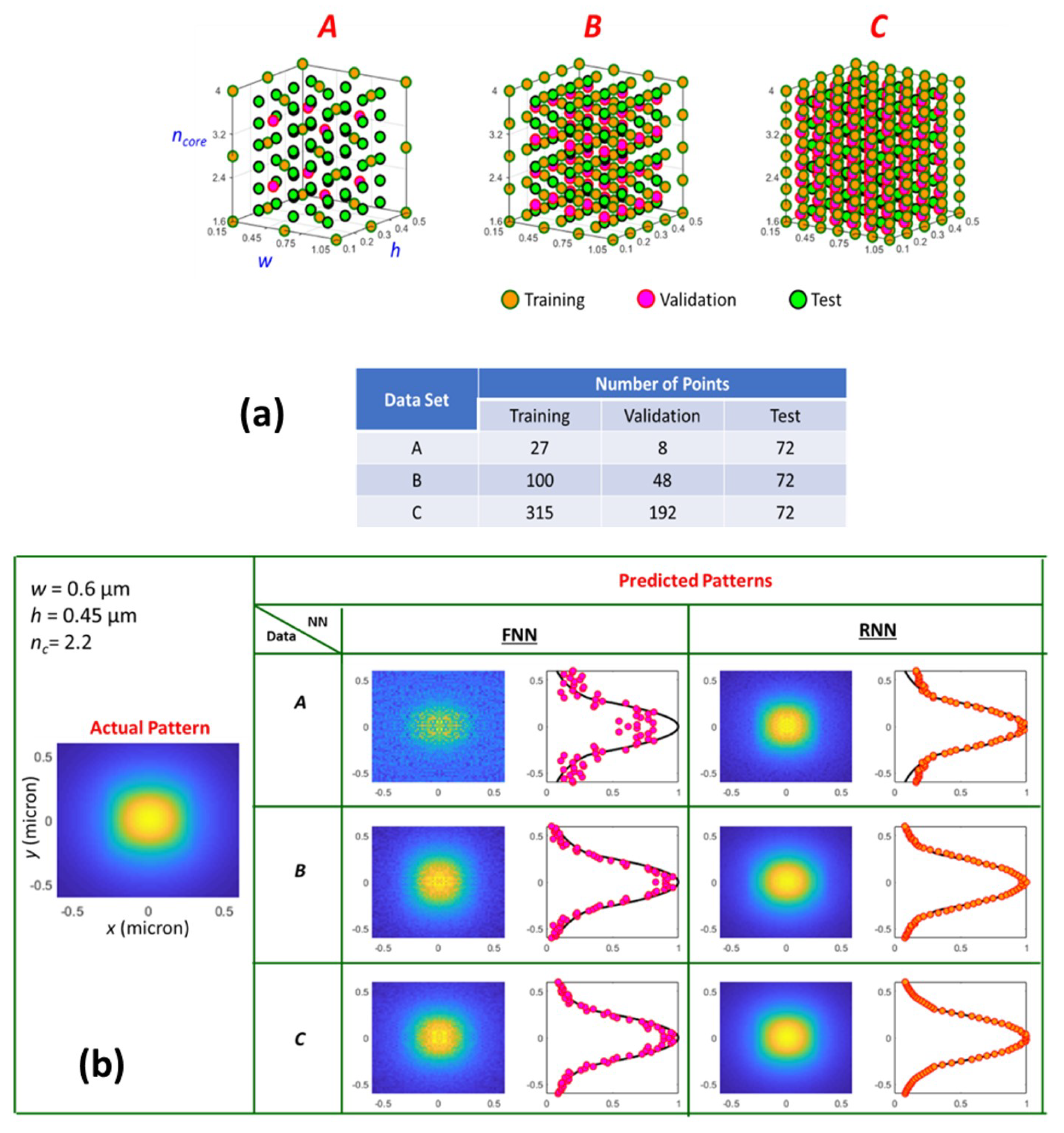
2.2.3. Optical Mode Profile

Apart from modal classifications and effective refractive index calculations, another essential task in integrated photonics is the calculation of the optical mode profiles. Unlike effective refractive index prediction, where the task is to predict a single value for a given waveguide geometry and polarization, here the deep-learning model must be able to predict a two-dimensional array of values corresponding to the distribution of the electric field. In [38], a recurrent neural network (RNN) was employed to accomplish this task. The input to the model is the geometrical parameters of the waveguide, and the output is the field values (array). The recurrent connection helps to establish the field continuity between the adjacent pixels. Figure 5 summarizes the key results.

2.3. Inverse Design of Photonic Structures: Deep Generative Models

In recent years, the deep learning (DL) has gained momentum in the design of photonics structures. Deep neural networks (DNNs) outperform established methods in discovering new photonics structures from massive data to achieve optimal optical performance. In this part, we review deep generative models (DGMs) for the inverse design of photonics structures, providing some insights as to how these deep generative models can solve the inverse design problems. We then provide a discussion on the current limitations and future directions of using DGMs for the inverse design of photonics structures.
DGMs are the methods combined generative models with DNNs, and they have achieved great success in only few years. The DGMs leverage the DNNs to learn a function that is capable of approximating the model distribution to the true data distribution of the training set so that new data points are generated with some variations. Generative Adversarial Nets (GANs) [53], variational autoencoders (VAEs) [60], and auto-regressive models [61] are popular DGMs, with the former two most commonly used.
GANs have been applied to the inverse design of metasurface nanostructures [62] and dielectric metasurfaces [63]. VAEs have been employed to the inverse design of double-layered chiral metamaterials [64]. GANs and VAEs mainly differ in the way of training generative models, but GANs produce better results as compared to VAEs. GANs introduces a novel way to train generative models. They consist of a generator G and a discriminator D, with G and D being trained in an adversarial manner. G generates a structure pattern x = G(z) from a random noise vector z, and D classifies the pattern x as synthesized (from G) or real (from training data). G attempts to fool D by producing patterns that cannot be distinguished from the ones in the training data. D is discarded once the networks are trained. Conditional GANs (cGANs) are the most widely used variation of GANs, that are constructed by simply adding conditional vector along with the noise vector. The inverse design of photonics structures requires that G outputs a structure pattern with desired optical response rather than a pattern generated randomely from random sample of noise z. cGANs are the way to do that. By conditioning G on target response y so that G outputs a reconstruction x ^ = G(y). An ANN based metamodel was trained to approximate the optical and chromatic response of a hybrid subwavelength grating (HSWG) structure [65]. It can serve as a surrogate model for fast spectral performance prediction in the cGANs for inverse design. Deep Convolutional GANs (DCGANs) are the GANs employing Convolutional Neural Network (CNN) architecture. They are comprised of many convolutional, deconvolutional and fully connected layers.
There are problems with GANs and one of them is stabilizing their training. The accuracy of the generative model depends on both the number and quality of training data. However GANs are indeed powerful, being used in a variety of tasks. Unifying GANs and VAEs allows obtaining the best of both models. In the next few years, DGMs will be very helpful for the inverse design of various photonics devices.

3. Photonics for AI: Using Photonics Computing to Implement AI Algorithms

In the previous sections, we investigated how AI algorithms, such as deep learning, can be utilized in the design and optimization of photonics devices [33,66]. Here, we will review some of the recent research work in photonics computing that demonstrates how photonics systems are used to implement the AI algorithms. There is, thus, a strong synergy between photonics and AI: AI can be used to accelerate the design process of photonics devices, and photonics, in turn, can be used to implement the AI algorithms and to boost the performance of the AI systems due to some of the inherent advantages of photonics, such as lower latency compared with electronics.
Artificial intelligence—in particular, deep learning [67]—brought about a step-function improvement in image classification in the early 2010s and has since made a much deeper and broader influence on how businesses and organizations operate [68]. Studies project that AI will massively impact the global economy in the 2020s as a result of increased productivity in almost all industry sectors [69]. We can expect to see major investment from both the public and private sector and a shift towards an “AI first” strategy [70], where AI techniques will be adopted to improve outcomes beyond traditional techniques.
The success of deep learning has been attributed to the convergence of three important factors: (1) advances in deep learning research, (2) access to large high quality datasets, and (3) the advent of hardware deep learning accelerators. GPUs and ASICs (e.g., TPUs [71]), which are special purpose hardware for machine learning applications, have been deployed in data centers for nearly 5 years. Worryingly, a study in 2018 by OpenAI highlighted the astonishing growth of compute resources used by AI, showing a 3.5 month doubling time, which was faster than Moore’s law [72]. Moreover, Moore’s law scaling is expected to end within the next decade due to fundamental limits to transistor scaling as well as related bottlenecks in power dissipation and interconnect bandwidth [73]. The study called into question the economic and environmental sustainability of the exponential growth of compute demand and underscored the need to consider non-conventional computing architectures to continue to drive future innovations in AI.
At the same time, integrated silicon photonics has made significant advances over the past decade. The performance of silicon photonics devices and systems continues to improve, driven mainly by high bandwidth requirements from tele-communications and data center interconnects applications [74,75]. Silicon photonics foundry fabrication processes are also becoming more mature and reliable [76,77], such that the community is looking to develop applications beyond data interconnects, for example LIDAR [78], quantum computing [79] and in particular, machine learning and neuromorphic computing [80,81].
Using photonics for deep learning and neuromorphic computing has many potential advantages over conventional electronics, namely, large bandwidth, low latency, and nearly lossless interconnects [82]. Moreover, spatial and wavelength multiplexing enables high speed high throughput information processing, e.g., the multiplication and summation of signals, which is a critical operation in deep learning.

3.1. Current Developments in Photonics Computing

Most hardware machine learning accelerators currently in deployment are high-throughput parallel processors, like GPUs and TPUs. Research into non von Neumann architectures like neuromorphic computing, in which aspects of the design mimic principles present in biological neural networks, is ongoing. Among these, the memristor crossbar array stands out as a promising candidate [83]. Multiplication and summation is implemented following Ohm’s law at each cross-point and Kirchhoff’s current law at each column. However, engineering challenges remain as the variability and non-ideal characteristic of memristive devices make large scale arrays difficult to realise. Nonetheless, several impressive recent demonstrations indicate progress towards scalability [84,85]. On the other hand, several studies have projected that the fundamental limits of analog optical computing are on equal footing or even slightly advantageous when compared to memristors [86,87].
Early studies on optical computing and optical neural networks date back to the late 1980s [88,89], and the technology was touted to enable a new generation of faster computers [90]. Inopportunely, the first optical neural networks were implemented with bulk optical components, which are large, slow and unstable and, hence, were unfeasible to scale to large and densely connected networks. Decades of major breakthroughs in integrated electronics manufacturing has led to its dominance in computing today and a circumspect view of the prospects of computing with optics [91]. However, the limits of continued transistor scaling and recent developments in integrated silicon photonics has breathed new life into the field of optical information processing. Advances in silicon photonics foundry processes has enabled demonstrations of high-speed silicon photonics integrated circuits with thousands of elements with reconfigurable functions [92,93]. Leveraging on the silicon photonics technology platform, several research groups, start-ups and large companies have begun work on optical neural networks over the latter part of the last decade. Table 2 shows a summary of proposed and demonstrated photonics neural network architectures from recent published works. We give an overview of these different architectures in Section 4.

3.2. Photonic Accelerator

Matrix multiplications are one of the most common operations in high performance computing. In fact, current deep-learning models rely heavily on computing matrix multiplications, but conventional computers using the von Neumann architecture are not optimized for such calculations. Data and instructions need to be moved over metal line interconnects from the memory cache to the CPU (or matrix multiplication units) and back. Moreover, metal lines have to be charged and discharged at energy cost of CV 2 [82]. Thus, conventional electronic computers suffer from high communication overheads and high latencies. On the other hand, linear transformations, including matrix computations [112] and Fourier transforms [113], can be performed with high speed and high throughput using photonics—typically orders of magnitude better than electronics [86,87]. For example, photonics devices typically have bandwidth of 20 GHz and the propagation delay through a photonics chip is on order of 100 ps. In view of these advantages, there have been several published works on using photonics as co-processors to accelerate expensive and time consuming computations [94,95,96,97,98]. Indeed, several high profile startups are currently working on photonics chips as drop-in replacements for electronic deep learning accelerators like TPUs [114,115,116]. The great interest from industry indicates the near term promise of photonics accelerators. Ironically, the main bottlenecks for photonics accelerators are the periphery electronics. For example, the analog nature of the photonics computation requires low power and high bandwidth digital–analog and analog–digital conversion circuits and amplifier circuits for modulation and detection. Another challenge is that deep-learning models have to be adapted to be able to accept the low precision and potentially noisy analog computations [117,118,119]. Photonic accelerators are hybrid digital-analog systems, which makes sense when working with digital data. However, if the incoming data is inherently analog, for example in sensing applications, then all-optical neural network analog information processing that bypasses D/A and A/D conversions could have advantages.

3.3. Coherent Feed-Forward Neural Network

Implementations of optical neural networks can be generally classified as coherent or incoherent. Coherent circuits make use of constructive or destructive interference in multi-port interferometers to implement linear transformations like matrix multiplications. A very general interferometric device is a regular mesh of Mach–Zehnder interferometers (MZIs), which has been shown to be able to implement any unitary matrix [120]. Then, using singular value decomposition, real valued matrices that are used in most neural networks can be implemented [99]. Additionally, there are proposals to use these Mach–Zehnder interferometers to implement novel architectures, such as unitary neural networks [121] and quantum neural networks [122]. A major challenge for such coherent circuits is the sensitivity of the performance to fabrication imprecision and additional loss, with several groups proposing more robust designs [100,101]. This requires O(N 2 ) MZIs to implement a N×N square matrix, which limits the maximum possible network size on a chip. Furthermore, integrating all-optical nonlinear activations into the coherent circuit remains an area of active research [96].

3.4. Continuous-Time Recurrent Neural Network

Incoherent circuits use non-interfering signal carriers (e.g., wavelengths, polarizations, modes) to perform weighted summations. One prominent architecture uses wavelength division multiplexing to collect and distribute signals weighted by micro-ring resonators [103]. The collected wavelengths are summed by photodetectors measuring the total power. The photodetector current then drives a modulator acting as a nonlinear node whose output is fed back into the network [104]. This kind of feedback network implements a continuous-time recurrent neural network. Implementing densely connected layer with N number of input and output nodes requires N 2 micro-ring resonators, which have to be individually thermally controlled as they are highly sensitive to inevitable fabrication imprecision. Additionally, N independent wavelength channels have to fit within one free-spectral range, which have to be sufficiently spaced to inhibit inter-channel cross-talk. These strict component requirements means that scaling up such an architecture faces severe challenges.

3.5. Spiking Neural Network with Phase-Change Materials

Another architecture uses waveguides embedded with phase-change materials, which can be switched between non-volatile multi-level transmission states by optical pulses [105]. The phase-change material thus stores the weight values of the neural network and also acts as a nonlinear activation function. Additionally, researchers were able to demonstrate a simplified spike-timing-dependent plasticity by overlapping pulses in time, to show unsupervised learning [106]. Recent demonstrations use wavelength division multiplexing micro-rings for signal collection, distribution and summation and hence face similar challenges as above. Phase change materials like GST-PCMs have a limited number of programmable states (3 bit) and hence are more desirable for low precision neural networks. Engineering phase change materials with low-switching powers and fast response times is on-going research. Furthermore, phase change materials, although technically “CMOS compatible”, are not currently standard in the photonics foundry process. Existing proposals advocate for the integration of phase change materials into the photonics platform [123], but it is unlikely to be a short term endeavor.

3.6. Reservoir Computing

Reservoir computing is a framework that is closely related to recurrent neural networks. The reservoir is a tunable nonlinear dynamical system with randomly interconnected nodes that takes input data and projects it into a high dimensional feature space. Predictions from the reservoir are a linear combination of the observed states of the reservoir obtained by linear regression. Recent demonstrations of photonics reservoirs include a network of spiral waveguides [107] and several proposals exist that use networks of micro-resonators [108,109]. Another proposed reservoir computer consists of a multi-modal optical waveguide, with the large number of optical modes acting as reservoir nodes and random coupling due to light scattering behaving as the random connectivity in the network [104,105]. Several challenges exist for scaling up photonics reservoirs, for example, loss accumulation in the reservoir. There is also difficulty in observing the node states to train the readout weights in an efficient manner.

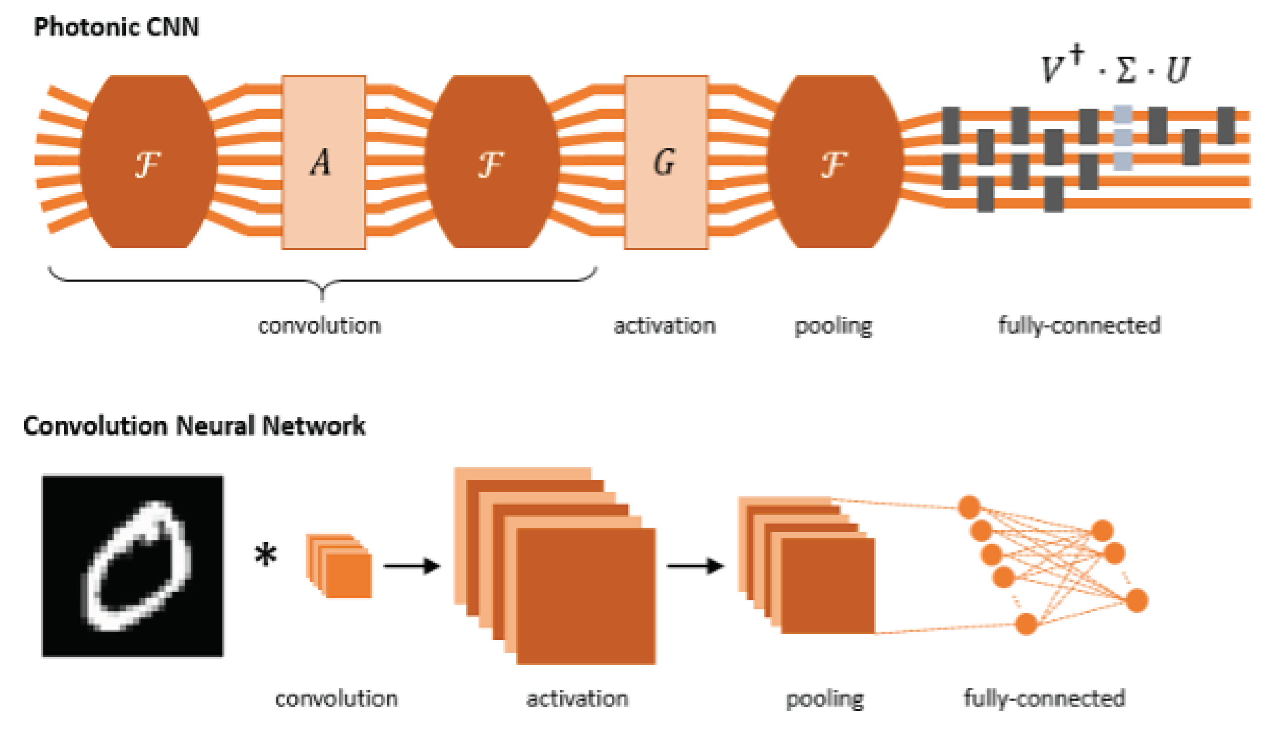
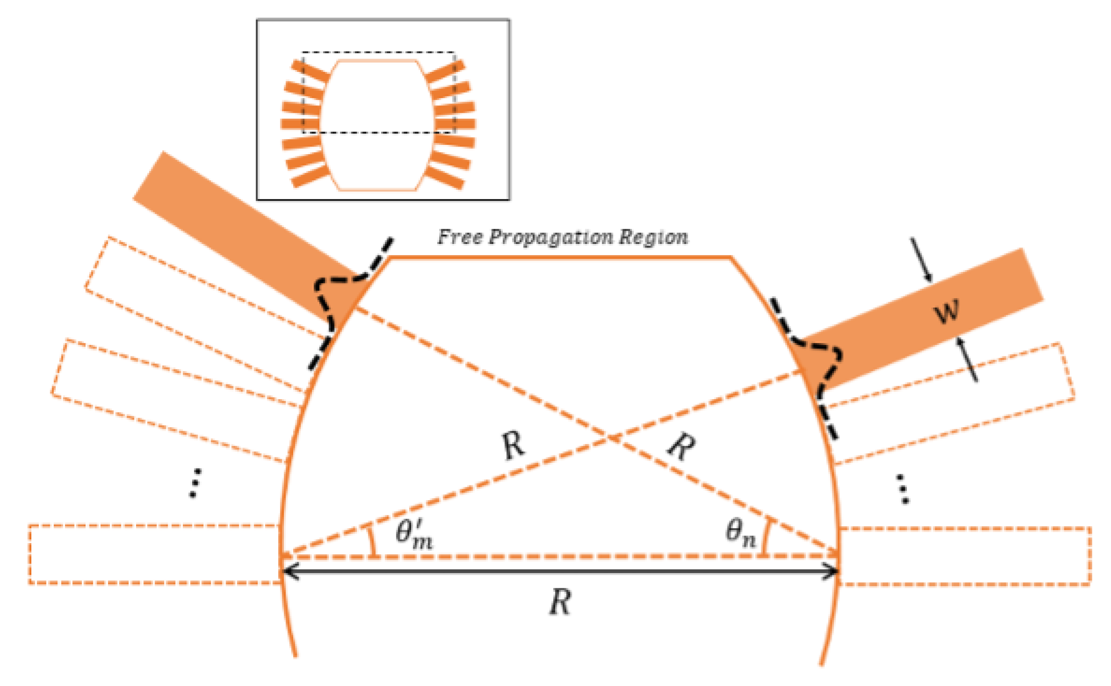
3.7. On-Chip Fourier Transform and Convolutions Using Star Couplers

In convolution neural networks (CNN), the convolution layer uses far fewer learned parameters than a fully connected layer, due to the shared weights architecture, while showing equal or better performance in classification tasks. CNNs are a promising approach for optical neural networks, as convolutions can be implemented with Fourier optics [113]. Additionally, the shared weights allow high performance while reducing the total required components. The generic model of a CNN and the implementation of such network photonics is illustrated in Figure 6.
We recently proposed the use of a N × N star coupler [124,125], as shown in Figure 7, which is a diffractive component, to perform the Fourier transform [113] and (by the convolution theorem) the convolution operation, to be used in convolutional neural networks (CNNs) [126]. To implement convolution, (1) a first star coupler will transform the input data to the Fourier space, (2) phase and/or amplitude modulators will apply the kernel filters, and (3) a second star coupler will transform the data back to configuration space. Compared to a typical MZI implementation of the (unitary) Fourier transform, our simulations predict a footprint reduction by tens of times when using the star coupler. This considerable reduction in footprint not only saves physical space on the chip but also reduces accumulated propagation loss as light has to travel a shorter distance, making deep neural networks feasible to be implemented using coherent photonics integrated circuits. Details of our work can be found in [126].

4. AI Beyond Photonics

Section 2 and Section 3 introduce how AI methods can help in photonics simulation and design, and how photonics, in turn, can help AI algorithms for acceleration. In addition to photonics, AI techniques have been widely applied in many other photonics-related fields, such as electromagnetics, quantum, etc. This section will briefly summarize the recent AI algorithms that have been applied to Computational Electromagnetic (CEM), RF components, Electromagnetic Compatibility (EMC) and Electromagnetic Interference (EMI), and quantum-related topics.

4.1. AI for Computational Electromagnetic Solvers: Forward and Inverse

The three most popular computational electromagnetic methods for solving forward electromagnetic problems are Finite-difference time-domain method (FDTD) [127], finite element method (FEM) [128], and method of moment (MoM) [129]. No matter which method is chosen, the differential and/or integral form of Maxwell’s equations, along with the computational domain, will be discretized into linear matrice. With the EM modeling becomes more complicated and larger, considerable computational resources and more computational time are required. To improve the computational efficiency at the cost of accuracy, AI techniques can be a good solution, especially when the forward EM problems need repetitive simulations.
For frequency-domain forward EM solver, machine-learning based MoM was reported to solve the static parasitic capacitance extraction and dynamic electromagnetics scattering problems [130,131]. Barmada et al. used trained CNN to output the boundary conditions (BCs) for the BC condition of a reduced finite-element method (FEM) model [132]. 1-D to 3-D Electrostatic problems based on Poisson equation solved by CNN instead of using FEM have been reported [133,134,135,136]. Additionally, Unet is a popularly used neural network for image processing, such as image segmentation [137], colorization [16], etc. It is reported that a 2D-Unet based Finite-difference Frequency-domain (FDFD) solver is employed to evaluate scattered EM fields and achieved 2000 times efficiency gain compared with conventional FDFD method [138].
For time-domain forward EM solvers, a recurrent convolutional neural network (RCNN), a neural network widely used in time series data, is used to replace FDTD solver for solving scattering problems [139], as the time-marching scheme is suitable for RNNs in nature. In [140,141], ML-based GPR forward solvers are used to simulate the ground penetrating radar in real time, trained by data generated using FDTD solver with tuning parameters including fractal dimension of water fraction, the height of the antenna, etc. Absorbing boundary, such as Mur and PML (CPML, UPML) are essential for most CEM methods. Without high-performance absorbing boundary, CEM methods are unable to solve various EM problems with truncated computational domain. However, the additional boundaries usually lead to the increase of the computational domain with additional artificial layers. Deep-learning-based methods are used to improve the efficiency of FDTD methods with absorbing boundaries [142,143,144].
However, most forward EM solvers using AI cannot solve general EM problems due to (1) most solvers are trained by limited data and the trained data are generated by limited parameters; (2) the trained AI model are constrained for some specific application/problem; (3) the accuracy is low compared with full-wave solvers, especially when the training data is limited. On the other hand, many AI techniques for EM inverse scattering problems (ISP) [145] are reported and show great improvement in both accuracy and efficiency [22]. Similar to the topics of inverse problems in image processing topics, AI methods are suitable for various ISP by nature. Chen et al. summarize the state-of-the-art methods of solving ISPs with deep learning methods in the review paper [22] and discuss how to combine neural networks with knowledge of the underlying physics as well as traditional non-learning techniques.

4.2. AI for Microwave Devices: Design, Optimization, and Applications

Microwave Devices, such as antenna, filters, and amplifiers are the most common RF components used in wireless communication systems. With the development of advanced semiconductor techniques, more and more compact microwave devices are demanded to integrate with the other wireless communication devices. Thus, the microwave devices are designed with more complicated structures, smaller sizes and optimal performances, and the difficulty of simulation, optimization, and design has been dramatically increased accordingly. To this end, many researchers leverage AI to assist on the optimization and design of various microwave devices.
Optimization is usually the last phase of microwave device design, using AI techniques, such as ANNs for various EM-based designs has drawn much attention since 2004 [146]. Combining the time-domain solver, such as FDTD and Transmission Line Matrix (TLM) methods [147,148] with neural networks, the design of microwave devices can be optimized more efficiently. In order to optimize the microwaves devices efficiently, a fast-forward solver is usually required to avoid extensive simulations. To this end, AI can be applied to learn from a collection of simulated data to replace a time-consuming full-wave solver. In [149], ANN is adopted as the surrogate model to the time-consuming electromagnetic model to speed up the homotopy filter optimization process. A dual bandpass filter is designed using ANN to extract the filter transfer function [150]. In [151], DNN with smooth rectified linear unit (ReLU) activation function is proposed to extract the coupling matrix for multi-coupled cavity filter based on the desired S parameters. The smooth ReLU function avoids the discontinuity of the derivative of the DL model with the conventional ReLU function. In [152], DNN is used to obtain the S-parameters from geometrical variables of filters and the operating frequency. Unlike the methods using DNNs, Chen et al. extract the coupling matrix of fourth-order and sixth-order coupling filters using a manifold Gaussian process (MGP) ML method based on differential evolution (DE) algorithm [153]. Similarly, the forward simulation of slotted waveguide antenna [154], patch antenna [155], and planar inverted F-antenna (PIFA) [156] are reported as alternatives using DNNs at an acceptable cost of accuracy. In [157], a semi-supervised co-training algorithm based on Gaussian process (GP) and support vector machine (SVM) by using a few labeled samples to obtain a relatively high-precision surrogate model is proposed for the optimal design of Yagi microstrip antenna (MSA) and GPS Beidou dual-mode MSA.
Deep reinforcement learning (DRL) methods, one of the significant parts of deep learning method in recent years, have been applied in the automatical design of some microwave devices. Ohira et al. propose a deep Q-learning network (DQN) based fine-tuning method for bandpass filter design using two NNs by supervised learning. One of the two NNs is the forward model, also named as environment, for calculating the coupling matrix from the filter structural parameters [158]. The other is the inverse model based on DQN for tuning the filter by giving the optimal actions according to the reward for a certain state from the environment, named as agent. The discontinuous action space of the method is to change the structural parameters by increasing or decreasing 0.05 mm. Similarly, in [159], a double deep Q-learning (DDQN) approach is proposed to fine tune microwave cavity filters. DQN is one of the value-based methods in DRL. In addition to value-based DRL, another class of the DRL method is the policy gradient method. Wang et al. [160] present a framework based on deep deterministic policy gradient for tuning cavity filters, where continuous action space is valid. The Experience Replay and the Target Network of DQN is preserved to ensure the stability of the algorithm based on their previous work [161]. Unlike tuning the limited filter parameters, such as width and length of resonators, Liu et al. [12] developed a relational induction neural network (RINN) as the agent of the DRL method. Microwave components, such as filters and antennas can be designed with curved shapes and achieve the design goals, such as S-parameters and antenna gain. The structure of the microwave devices is defined as a set of parameterized mesh, and when each mesh changes, the simulation result is calculated by EM solvers, such as ADS or Ansys EM.
In addition to microwave devices, such as filters and antennas, some other microwave applications using AI have also been reported in power amplifier modeling [162,163], nonlinear microwave device modeling [164,165,166,167,168], microwave reflectometer design [169], beamforming design for 5G and MIMO system [170,171,172,173,174], and eddy current non-destructive testing [175,176].

4.3. AI for Electromagnetic Compatibility (EMC) and Electromagnetic Interference (EMI) Applications

The sky-rocketing increase in device complicity and operation frequency bring demands for machine learning (ML)-based techniques with groundbreaking efficiency improvement. The complex electromagnetic behavior in signal integrity (SI), power integrity (PI), and EMC make it difficult to categorized and describe the coupling nature with machine learning directly. Machine learning has been successfully facilitated in tackling EMC problems in many aspects with superior performance [20].
Machine learning is utilized in the performance evaluation of large-scale integrated circuits [177,178], and semiconductors [179]. Recently, a DNN-based macro modeling approach for the “black-box” problem [180] is proposed with the partial element equivalent circuit (PEEC) model [181]. ML also shows the capability in solving the optimization problems in EMI and SI/PI analysis [9,10]. In [182,183], the electromagnetic interference of PCB is analyzed by neural networks. The behavior of nonlinear circuit elements is predicted with a radial basis function neural network in [184]. Echo state networks and SVMs were proposed in [185,186] to model electromagnetic immunity of integrated circuits. A knowledge-based CNN is applied to establish and classify the entities to organized the EMC management [187]. In [188,189], the channel modeling and optimization are carried with an ANN to extract the lump circuit element matrix. Random-fuzzy uncertainty quantification is modeled with Bayesian optimization to propagate the uncertainty on the performance of the system [190]. The source reconstruction is essential while challenging for interference prediction in EMC, emission, and immunity analysis, which are formulated as regression problems governed by field integral equations. DNN, ANN, or generic [10,191,192] based algorithms are proposed with superior accuracy or efficiency.

4.4. AI for Quantum Related Topics

The development of AI, especially its subfield of ML, has revolutionized many areas in science and engineering. The research of AI and quantum photonics and beyond can be categorized into three parts: (1) quantum machine learning [193], which utilizes dedicated quantum computers as a new computing model to speed up machine learning; (2) utilization of machine learning to solve quantum physics problems [34,194]; (3) application of machine learning in the development of quantum devices and quantum computers. The review focuses on the third part. The methodology to utilize machine learning methods in design and optimization of photonics devices [195] has been reviewed in the previous sections. The sub-section will further discuss the application of machine learning in quantum control and quantum information processing.
Quantum systems are controlled by unitary operations engineered by a set of physical operations on the quantum systems. Quantum control enables quantum devices to perform the physical operations for information processing and quantum computation. To efficiently manipulate the quantum devices and programmable quantum computers, a large set of unitary operations has to be designed to control the devices to perform intended operations or stay in intended quantum states. This is a non-trivial task as the superposition of quantum state spans in a continues space with limited driving options in general. Haug et al. demonstrates an approach to prepare a continuous set of quantum states using deep reinforcement learning [196]. In order to achieve a robust control to qubits or gate operations, designed control protocol has to consider potential noises coming from the qubit environment or the control and readout processes. Wise et al. utilizes deep learning to extract the noise spectrum associated with a qubit surrounded by an arbitrary bath and mitigate the impact of qubit noise environment in the development of dynamical decoupling protocols [197]. For given noise models, August and Ni trains a recurrent neural network to optimize the sequences of dynamical decoupling to suppress errors in quantum memory [198]. Kim et al. uses neural networks to infer the amount of probability adjustment on the measurement and improve the accuracy of noisy intermediate-scale quantum (NISQ) algorithms without relying on extensive error characterization [199].
With the development of cloud-based quantum computing hardware [200,201], variational quantum-based algorithms (VQAs) [202], such as variational quantum eigensolver (VQE) have emerged as a promising candidate to achieve a practical quantum advantage over classical algorithms [203,204]. However, it is too challenging to run advanced deep neural networks over the existing quantum computing platforms due to the intractability of deep quantum circuits. Chen et al. [205] showed a proof-of-principle demonstration of variational quantum circuits to approximate the deep Q-value function of a DQN deep reinforcement learning. Lockwood and Si [206] explored pure and hybrid quantum algorithms for DQN and Double DQN, and found both hybrid and pure quantum variational circuit can solve reinforcement learning tasks with a smaller parameter space. With the development of quantum techniques, it is expected that more and more AI methods could be used in super-fast quantum computers.

5. Conclusions

AI has become a heated focus in and beyond photonics research in the past few years. As we have discussed in this review article, photonics benefits a great deal from AI for efficient soft computing and inverse design. Meanwhile, AI, in turn, benefits from photonics by carrying out AI algorithms, such as complicated deep neural networks using photonics components that use photons rather than electrons. We introduced the applications of AI on photonics modeling, simulation using soft computing, and inverse design based on a GAN model. Beyond the photonics domain, the other related research areas or topics governed by Maxwell’s equations share remarkable similarities in using the help of AI. The studies in computational electromagnetics, the design of microwave devices, EMC/EMI, and quantum computing greatly benefit from AI. We investigated the applications of AI for the forward and inverse CEM methods, the modeling and simulation of RF components (antennas, filters, etc.) and EMC/EMI problems using deep-learning models, inverse RF component design based on deep reinforcement learning, and a brief introduction on the recent AI techniques for quantum fields. We believe the relationship between AI and physics will continue to flourish in a mutually advancing manner both in photonics and beyond.

Author Contributions

Conceptualization, C.E.P., G.A., J.R.O., Z.Y. and T.Y.L.A.; methodology, G.A., J.R.O., Z.Y., T.Y.L.A., W.Z. (Weijiang Zhao), Y.J., W.Z. (Wenzu Zhang) and C.E.P.; writing—original draft preparation, G.A., J.R.O., Z.Y., T.Y.L.A., W.Z. (Weijiang Zhao), Y.J. and W.Z. (Wenzu Zhang); writing—review and editing, C.E.P., G.A., Z.Y. and T.Y.L.A.; supervision, C.E.P. All authors have read and agreed to the published version of the manuscript.

Funding

This work is supported by RGANS1901, “AI-Enabled Electronic-Photonic IC Design”. This work is also supported by the A*STAR RIE2020 Advanced Manufacturing and Engineering (AME) Programmatic Fund [A20H5g2142].

Institutional Review Board Statement

Not applicable.

Informed Consent Statement

Not applicable.

Data Availability Statement

Not applicable.

Conflicts of Interest

The authors declare no conflict of interest.

Abbreviations

The following abbreviations are used in this manuscript:
AIArtificial Intelligence
ANNArtificial Neural Networks
CEMComputational Electromagnetics
CNNConvolutional Neural Network
cGANConditional Generative Adversarial Network
DLDeep Learning
DNNDeep Neural Networks
DGMDeep Generative Model
DCGANDeep Convolutional Generative Adversarial Network
DRLDeep Reinforcement Learning
DQNDeep Q-learning Network
DDQNDouble Deep Q-learning Network
DEDifferential Evolution
EMElectromagnetics
EMCElectromagnetic Compatibility
EMIElectromagnetic Interference
FDTDFinite-Difference Time-Domain
FDFDFinite-Difference Frequency-Domain
FEMFinite Element Method
GANGenerative Adversarial Network
GPGaussian Process
ISPInverse Scattering Problems
MOMMethod of Moment
MLMachine Learning
NNNeural Network
NLPNatural Language Processing
NISQNoisy Intermediate-Scale Quantum
PEECPartial Element Equivalent Circuit
RFRadiofrequency
RNNRecurrent Neural Network
ReLURectified Linear Unit
RLReinforcement Learning
SVMSupport Vector Machine
TLMTransmission-Line Matrix
VAEVariational Autoencoder
VQAVariational Quantum-Based Algorithm
VQEVariational Quantum Eigensolver

References

  1. Kong, J.A. Theory of Electromagnetic Waves; Wiley-Interscience: New York, NY, USA, 1975. [Google Scholar]
  2. Ulaby, F.T.; Michielssen, E.; Ravaioli, U. Fundamentals of Applied Electromagnetics; Pearson Boston: Boston, MA, USA, 2015. [Google Scholar]
  3. Hayt, W.H., Jr.; Buck, J.A.; Akhtar, M.J. Engineering Electromagnetics|(SIE); McGraw-Hill Education: New York, NY, USA, 2020. [Google Scholar]
  4. Tsang, L.; Kong, J.A.; Ding, K.H. Scattering of Electromagnetic Waves: Theories And applications; John Wiley & Sons: Hoboken, NJ, USA, 2004; Volume 27. [Google Scholar]
  5. Pozar, D.M. Microwave Engineering; John Wiley & Sons: Hoboken, NJ, USA, 2011. [Google Scholar]
  6. Hecht, E. Optics, 5th ed.; Pearson: London, UK, 2017. [Google Scholar]
  7. Boyd, R.W. Nonlinear Optics; Academic Press: Cambridge, MA, USA, 2020. [Google Scholar]
  8. Saleh, B.E.; Teich, M.C. Fundamentals of Photonics; John Wiley & Sons: Hoboken, NJ, USA, 2019. [Google Scholar]
  9. Shi, D.; Wang, N.; Zhang, F.; Fang, W. Intelligent electromagnetic compatibility diagnosis and management with collective knowledge graphs and machine learning. IEEE Trans. Electromagn. Compat. 2020, 63, 443–453. [Google Scholar] [CrossRef]
  10. Huang, Q.; Fan, J. Machine learning based source reconstruction for RF desense. IEEE Trans. Electromagn. Compat. 2018, 60, 1640–1647. [Google Scholar] [CrossRef]
  11. Ohira, M.; Takano, K.; Ma, Z. A Novel Deep-Q-Network-Based Fine-Tuning Approach for Planar Bandpass Filter Design. IEEE Microw. Wirel. Components Lett. 2021, 31, 638–641. [Google Scholar] [CrossRef]
  12. Liu, J.; Chen, Z.X.; Dong, W.H.; Wang, X.; Shi, J.; Teng, H.L.; Dai, X.W.; Yau, S.S.T.; Liang, C.H.; Feng, P.F. Microwave integrated circuits design with relational induction neural network. arXiv 2019, arXiv:1901.02069. [Google Scholar]
  13. Bulgarevich, D.S.; Talara, M.; Tani, M.; Watanabe, M. Machine learning for pattern and waveform recognitions in terahertz image data. Sci. Rep. 2021, 11, 1–8. [Google Scholar]
  14. Cao, Z.; Yang, H.; Zhao, J.; Pan, X.; Zhang, L.; Liu, Z. A new region proposal network for far-infrared pedestrian detection. IEEE Access 2019, 7, 135023–135030. [Google Scholar] [CrossRef]
  15. Denholm, S.; Brand, W.; Mitchell, A.; Wells, A.; Krzyzelewski, T.; Smith, S.; Wall, E.; Coffey, M. Predicting bovine tuberculosis status of dairy cows from mid-infrared spectral data of milk using deep learning. J. Dairy Sci. 2020, 103, 9355–9367. [Google Scholar] [CrossRef]
  16. Yang, Z.; Chen, Z. Learning From Paired and Unpaired Data: Alternately Trained CycleGAN for Near Infrared Image Colorization. In Proceedings of the 2020 IEEE International Conference on Visual Communications and Image Processing (VCIP), Macau, China, 1–4 December 2020; pp. 467–470. [Google Scholar]
  17. Chen, J.; Hou, J.; Ni, Y.; Chau, L.P. Accurate light field depth estimation with superpixel regularization over partially occluded regions. IEEE Trans. Image Process. 2018, 27, 4889–4900. [Google Scholar] [CrossRef] [Green Version]
  18. Chen, J.; Hou, J.; Chau, L.P. Light field compression with disparity-guided sparse coding based on structural key views. IEEE Trans. Image Process. 2017, 27, 314–324. [Google Scholar] [CrossRef] [Green Version]
  19. Lai, P.Y.; Liu, H.; Ng, R.J.H.; Wint Hnin Thet, B.; Chu, H.S.; Teo, J.W.R.; Ong, Q.; Liu, Y.; Png, C.E. Investigation of SARS-CoV-2 inactivation using UV-C LEDs in public environments via ray-tracing simulation. Sci. Rep. 2021, 11, 1–10. [Google Scholar]
  20. Massa, A.; Marcantonio, D.; Chen, X.; Li, M.; Salucci, M. DNNs as applied to electromagnetics, antennas, and propagation—A review. IEEE Antennas Wirel. Propag. Lett. 2019, 18, 2225–2229. [Google Scholar] [CrossRef]
  21. Erricolo, D.; Chen, P.Y.; Rozhkova, A.; Torabi, E.; Bagci, H.; Shamim, A.; Zhang, X. Machine learning in electromagnetics: A review and some perspectives for future research. In Proceedings of the 2019 International Conference on Electromagnetics in Advanced Applications (ICEAA), Granada, Spain, 9–13 September 2019; pp. 1377–1380. [Google Scholar]
  22. Chen, X.; Wei, Z.; Li, M.; Rocca, P. A review of deep learning approaches for inverse scattering problems (invited review). Prog. Electromagn. Res. 2020, 167, 67–81. [Google Scholar] [CrossRef]
  23. He, K.; Zhang, X.; Ren, S.; Sun, J. Deep residual learning for image recognition. In Proceedings of the IEEE Conference on Computer Vision and Pattern Recognition, Las Vegas, NV, USA, 27–30 June 2016; pp. 770–778. [Google Scholar]
  24. Lu, D.; Weng, Q. A survey of image classification methods and techniques for improving classification performance. Int. J. Remote Sens. 2007, 28, 823–870. [Google Scholar] [CrossRef]
  25. Jiao, L.; Zhao, J. A Survey on the New Generation of Deep Learning in Image Processing. IEEE Access 2019, 7, 172231–172263. [Google Scholar] [CrossRef]
  26. Chen, J.; Tan, C.H.; Hou, J.; Chau, L.P.; Li, H. Robust video content alignment and compensation for rain removal in a cnn framework. In Proceedings of the IEEE Conference on Computer Vision and Pattern Recognition, Salt Lake City, UT, USA, 18–23 June 2018; pp. 6286–6295. [Google Scholar]
  27. Chowdhury, G.G. Natural language processing. Annu. Rev. Inf. Sci. Technol. 2003, 37, 51–89. [Google Scholar] [CrossRef] [Green Version]
  28. Huang, Z.; Xu, W.; Yu, K. Bidirectional LSTM-CRF models for sequence tagging. arXiv 2015, arXiv:1508.01991. [Google Scholar]
  29. Lillicrap, T.P.; Hunt, J.J.; Pritzel, A.; Heess, N.; Erez, T.; Tassa, Y.; Silver, D.; Wierstra, D. Continuous control with deep reinforcement learning. arXiv 2015, arXiv:1509.02971. [Google Scholar]
  30. Gu, S.; Holly, E.; Lillicrap, T.; Levine, S. Deep reinforcement learning for robotic manipulation with asynchronous off-policy updates. In Proceedings of the 2017 IEEE international conference on robotics and automation (ICRA), Singapore, 29 May–3 June 2017; pp. 3389–3396. [Google Scholar]
  31. Waltman, V.E. VOSviewer. Available online: www.vosviewer.com (accessed on 20 November 2021).
  32. Jiang, J.; Chen, M.; Fan, J.A. Deep neural networks for the evaluation and design of photonic devices. Nat. Rev. Mater. 2021, 6, 679–700. [Google Scholar] [CrossRef]
  33. Ma, W.; Liu, Z.; Kudyshev, Z.A.; Boltasseva, A.; Cai, W.; Liu, Y. Deep learning for the design of photonics structures. Nat. Photonics 2021, 15, 77–90. [Google Scholar] [CrossRef]
  34. Pfau, D.; Spencer, J.S.; Matthews, A.G.; Foulkes, W.M.C. Ab initio solution of the many-electron Schrödinger equation with deep neural networks. Phys. Rev. Res. 2020, 2, 033429. [Google Scholar] [CrossRef]
  35. Malkiel, I.; Mrejen, M.; Nagler, A.; Arieli, U.; Wolf, L.; Suchowski, H. Plasmonic nanostructure design and characterization via deep learning. Light. Sci. Appl. 2018, 7, 1–8. [Google Scholar] [CrossRef] [PubMed]
  36. Alagappan, G.; Png, C.E. Universal deep learning representation of effective refractive index for photonics channel waveguides. JOSA B 2019, 36, 2636–2642. [Google Scholar] [CrossRef]
  37. Wiecha, P.R.; Muskens, O.L. Deep learning meets nanophotonics: A generalized accurate predictor for near fields and far fields of arbitrary 3D nanostructures. Nano Lett. 2019, 20, 329–338. [Google Scholar] [CrossRef] [PubMed] [Green Version]
  38. Alagappan, G.; Png, C.E. Prediction of electromagnetic field patterns of optical waveguide using neural network. Neural Comput. Appl. 2021, 33, 2195–2206. [Google Scholar] [CrossRef]
  39. Lio, G.E.; Ferraro, A. LIDAR and Beam Steering Tailored by Neuromorphic Metasurfaces Dipped in a Tunable Surrounding Medium. In Photonics; Multidisciplinary Digital Publishing Institute: Basel, Switzerland, 2021; Volume 8, p. 65. [Google Scholar]
  40. Colburn, S.; Majumdar, A. Inverse design and flexible parameterization of meta-optics using algorithmic differentiation. Commun. Phys. 2021, 4, 1–11. [Google Scholar] [CrossRef]
  41. Nadell, C.C.; Huang, B.; Malof, J.M.; Padilla, W.J. Deep learning for accelerated all-dielectric metasurface design. Opt. Express 2019, 27, 27523–27535. [Google Scholar] [CrossRef]
  42. Inampudi, S.; Mosallaei, H. Neural network based design of metagratings. Appl. Phys. Lett. 2018, 112, 241102. [Google Scholar] [CrossRef]
  43. Liu, Z.; Feng, W.; Long, Y.; Guo, S.; Liang, H.; Qiu, Z.; Fu, X.; Li, J. A Metasurface Beam Combiner Based on the Control of Angular Respons. In Photonics; Multidisciplinary Digital Publishing Institute: Basel, Switzerland, 2021; Volume 8, p. 489. [Google Scholar]
  44. Pilozzi, L.; Farrelly, F.A.; Marcucci, G.; Conti, C. Machine learning inverse problem for topological photonics. Commun. Phys. 2018, 1, 1–7. [Google Scholar] [CrossRef]
  45. Cao, Y.; Li, S.; Petzold, L.; Serban, R. Adjoint sensitivity analysis for differential-algebraic equations: The adjoint DAE system and its numerical solution. SIAM J. Sci. Comput. 2003, 24, 1076–1089. [Google Scholar] [CrossRef] [Green Version]
  46. Hughes, T.W.; Minkov, M.; Williamson, I.A.; Fan, S. Adjoint method and inverse design for nonlinear nanophotonics devices. ACS Photonics 2018, 5, 4781–4787. [Google Scholar] [CrossRef] [Green Version]
  47. Minkov, M.; Williamson, I.A.; Andreani, L.C.; Gerace, D.; Lou, B.; Song, A.Y.; Hughes, T.W.; Fan, S. Inverse design of photonics crystals through automatic differentiation. ACS Photonics 2020, 7, 1729–1741. [Google Scholar] [CrossRef]
  48. Lio, G.E.; Ferraro, A.; Ritacco, T.; Aceti, D.M.; De Luca, A.; Giocondo, M.; Caputo, R. Leveraging on ENZ Metamaterials to Achieve 2D and 3D Hyper-Resolution in Two-Photon Direct Laser Writing. Adv. Mater. 2021, 33, 2008644. [Google Scholar] [CrossRef] [PubMed]
  49. Jiang, J.; Fan, J.A. Global optimization of dielectric metasurfaces using a physics-driven neural network. Nano Lett. 2019, 19, 5366–5372. [Google Scholar] [CrossRef] [PubMed] [Green Version]
  50. Jiang, J.; Sell, D.; Hoyer, S.; Hickey, J.; Yang, J.; Fan, J.A. Free-form diffractive metagrating design based on generative adversarial networks. ACS Nano 2019, 13, 8872–8878. [Google Scholar] [CrossRef] [PubMed] [Green Version]
  51. Mellit, A.; Eleuch, H.; Benghanem, M.; Elaoun, C.; Pavan, A.M. An adaptive model for predicting of global, direct and diffuse hourly solar irradiance. Energy Convers. Manag. 2010, 51, 771–782. [Google Scholar] [CrossRef]
  52. Yang, Z.; Hou, Y.; Chen, Z.; Zhang, L.; Chen, J. A Multi-Stage Progressive Learning Strategy for Covid-19 Diagnosis Using Chest Computed Tomography with Imbalanced Data. In Proceedings of the ICASSP 2021–2021 IEEE International Conference on Acoustics, Speech and Signal Processing (ICASSP), Toronto, ON, Canada, 6–11 June 2021; pp. 8578–8582. [Google Scholar] [CrossRef]
  53. Goodfellow, I.; Pouget-Abadie, J.; Mirza, M.; Xu, B.; Warde-Farley, D.; Ozair, S.; Courville, A.; Bengio, Y. Generative adversarial nets. Adv. Neural Inf. Process. Syst. 2014, 27. [Google Scholar]
  54. Creswell, A.; White, T.; Dumoulin, V.; Arulkumaran, K.; Sengupta, B.; Bharath, A.A. Generative adversarial networks: An overview. IEEE Signal Process. Mag. 2018, 35, 53–65. [Google Scholar] [CrossRef] [Green Version]
  55. Sherstinsky, A. Fundamentals of recurrent neural network (RNN) and long short-term memory (LSTM) network. Phys. D Nonlinear Phenom. 2020, 404, 132306. [Google Scholar] [CrossRef] [Green Version]
  56. Hochreiter, S.; Schmidhuber, J. Long short-term memory. Neural Comput. 1997, 9, 1735–1780. [Google Scholar] [CrossRef]
  57. Vaswani, A.; Shazeer, N.; Parmar, N.; Uszkoreit, J.; Jones, L.; Gomez, A.N.; Kaiser, Ł.; Polosukhin, I. Attention is all you need. In Proceedings of the IEEE Conference on Neural Information Processing Systems, Long Beach, CA, USA, 4–9 December 2017; pp. 6000–6010. [Google Scholar]
  58. Alagappan, G.; Png, C.E. Modal classification in optical waveguides using deep learning. J. Mod. Opt. 2019, 66, 557–561. [Google Scholar] [CrossRef]
  59. Alagappan, G.; Png, C.E. Deep learning models for effective refractive indices in silicon nitride waveguides. J. Opt. 2019, 21, 035801. [Google Scholar] [CrossRef]
  60. Kingma, D.P.; Welling, M. Auto-encoding variational bayes. arXiv 2013, arXiv:1312.6114. [Google Scholar]
  61. Larochelle, H.; Murray, I. The neural autoregressive distribution estimator. In Proceedings of the Fourteenth International Conference on Artificial Intelligence and Statistics, JMLR Workshop and Conference Proceedings, Ft. Lauderdale, FL, USA, 11–13 April 2011; pp. 29–37. [Google Scholar]
  62. Liu, Z.; Zhu, D.; Rodrigues, S.P.; Lee, K.T.; Cai, W. Generative model for the inverse design of metasurfaces. Nano Lett. 2018, 18, 6570–6576. [Google Scholar] [CrossRef] [PubMed] [Green Version]
  63. An, S.; Zheng, B.; Shalaginov, M.Y.; Tang, H.; Li, H.; Zhou, L.; Ding, J.; Agarwal, A.M.; Rivero-Baleine, C.; Kang, M.; et al. Deep learning modeling approach for metasurfaces with high degrees of freedom. Opt. Express 2020, 28, 31932–31942. [Google Scholar] [CrossRef]
  64. Ma, W.; Cheng, F.; Liu, Y. Deep-learning-enabled on-demand design of chiral metamaterials. ACS Nano 2018, 12, 6326–6334. [Google Scholar] [CrossRef]
  65. Es-saidi, S.; Blaize, S.; Macías, D. Hybrid modes and hybrid metastructures for color reproduction. In Hybrid Flatland Metastructures; Caputo, R., Lio, G.E., Eds.; AIP Publishing: Melville, NY, USA, 2021; pp. 5-1–5-18. [Google Scholar]
  66. Pilozzi, L.; Farrelly, F.A.; Marcucci, G.; Conti, C. Topological nanophotonics and artificial neural networks. Nanotechnology 2021, 32, 142001. [Google Scholar] [CrossRef]
  67. LeCun, Y.; Bengio, Y.; Hinton, G. Deep learning. Nature 2015, 521, 436–444. [Google Scholar] [CrossRef]
  68. Industry 4.0: From Big Data, AI, Robotics, to 3D Printing—Partnerships Are Key. Available online: https://www.edb.gov.sg/en/news-and-events/insights/manufacturing/industry-4-from-big-data-ai-robotics-to-3d-printing-partnerships-are-key.html (accessed on 7 February 2020).
  69. PwC’s Global Artificial Intelligence Study: Sizing the Prize. Available online: https://www.pwc.com/gx/en/issues/data-and-analytics/publications/artificial-intelligence-study.html (accessed on 7 February 2020).
  70. Making AI Work for Everyone. 17 May 2017. Available online: https://blog.google/technology/ai/making-ai-work-for-everyone/ (accessed on 7 February 2020).
  71. Jouppi, N.; Young, C.; Patil, N.; Patterson, D. Motivation for and evaluation of the first tensor processing unit. IEEE Micro 2018, 38, 10–19. [Google Scholar] [CrossRef]
  72. AI and Compute, OpenAI. 16 May 2018. Available online: https://openai.com/blog/ai-and-compute/ (accessed on 7 February 2020).
  73. Cavin, R.K.; Lugli, P.; Zhirnov, V.V. Science and engineering beyond Moore’s law. Proc. IEEE 2012, 100, 1720–1749. [Google Scholar] [CrossRef]
  74. Driscoll, J.B.; Doussiere, P.; Islam, S.; Narayan, R.; Lin, W.; Mahalingam, H.; Park, J.S.; Lin, Y.; Nguyen, K.; Roelofs, K.; et al. First 400G 8-channel CWDM silicon photonics integrated transmitter. In Proceedings of the 2018 IEEE 15th International Conference on Group IV Photonics (GFP), Cancun, Mexico, 29–31 August 2018; pp. 1–2. [Google Scholar]
  75. Maniloff, E.; Gareau, S.; Moyer, M. 400G and beyond: Coherent evolution to high-capacity inter data center links. In Proceedings of the 2019 Optical Fiber Communications Conference and Exhibition (OFC), San Diego, CA, USA, 3–7 March 2019; pp. 1–3. [Google Scholar]
  76. Lim, A.E.J.; Song, J.; Fang, Q.; Li, C.; Tu, X.; Duan, N.; Chen, K.K.; Tern, R.P.C.; Liow, T.Y. Review of silicon photonics foundry efforts. IEEE J. Sel. Top. Quantum Electron. 2013, 20, 405–416. [Google Scholar] [CrossRef]
  77. Sacher, W.D.; Huang, Y.; Lo, G.Q.; Poon, J.K. Multilayer silicon nitride-on-silicon integrated photonics platforms and devices. J. Light. Technol. 2015, 33, 901–910. [Google Scholar] [CrossRef]
  78. Poulton, C.V.; Byrd, M.J.; Russo, P.; Timurdogan, E.; Khandaker, M.; Vermeulen, D.; Watts, M.R. Long-range LiDAR and free-space data communication with high-performance optical phased arrays. IEEE J. Sel. Top. Quantum Electron. 2019, 25, 1–8. [Google Scholar] [CrossRef]
  79. Qiang, X.; Zhou, X.; Wang, J.; Wilkes, C.M.; Loke, T.; O’Gara, S.; Kling, L.; Marshall, G.D.; Santagati, R.; Ralph, T.C.; et al. Large-scale silicon quantum photonics implementing arbitrary two-qubit processing. Nat. Photonics 2018, 12, 534–539. [Google Scholar] [CrossRef] [Green Version]
  80. Peng, H.T.; Nahmias, M.A.; De Lima, T.F.; Tait, A.N.; Shastri, B.J. Neuromorphic photonics integrated circuits. IEEE J. Sel. Top. Quantum Electron. 2018, 24, 1–15. [Google Scholar] [CrossRef]
  81. Kitayama, K.i.; Notomi, M.; Naruse, M.; Inoue, K.; Kawakami, S.; Uchida, A. Novel frontier of photonics for data processing—Photonic accelerator. APL Photonics 2019, 4, 090901. [Google Scholar] [CrossRef] [Green Version]
  82. Miller, D.A. Attojoule optoelectronics for low-energy information processing and communications. J. Light. Technol. 2017, 35, 346–396. [Google Scholar] [CrossRef] [Green Version]
  83. Xia, Q.; Yang, J.J. Memristive crossbar arrays for brain-inspired computing. Nat. Mater. 2019, 18, 309–323. [Google Scholar] [CrossRef]
  84. Ambrogio, S.; Narayanan, P.; Tsai, H.; Shelby, R.M.; Boybat, I.; Di Nolfo, C.; Sidler, S.; Giordano, M.; Bodini, M.; Farinha, N.C.; et al. Equivalent-accuracy accelerated neural-network training using analogue memory. Nature 2018, 558, 60–67. [Google Scholar] [CrossRef]
  85. Yao, P.; Wu, H.; Gao, B.; Tang, J.; Zhang, Q.; Zhang, W.; Yang, J.J.; Qian, H. Fully hardware-implemented memristor convolutional neural network. Nature 2020, 577, 641–646. [Google Scholar] [CrossRef]
  86. Hamerly, R.; Bernstein, L.; Sludds, A.; Soljačić, M.; Englund, D. Large-scale optical neural networks based on photoelectric multiplication. Phys. Rev. X 2019, 9, 021032. [Google Scholar] [CrossRef] [Green Version]
  87. Nahmias, M.A.; De Lima, T.F.; Tait, A.N.; Peng, H.T.; Shastri, B.J.; Prucnal, P.R. Photonic multiply-accumulate operations for neural networks. IEEE J. Sel. Top. Quantum Electron. 2019, 26, 1–18. [Google Scholar] [CrossRef]
  88. Caulfield, H.J.; Kinser, J.; Rogers, S.K. Optical neural networks. Proc. IEEE 1989, 77, 1573–1583. [Google Scholar] [CrossRef]
  89. Ambs, P. Optical Computing: A 60-Year Adventure. Adv. Opt. Technol. 2010. [Google Scholar] [CrossRef] [Green Version]
  90. Light May Be Key To New Generation of Fast Computers—The New York Times. Available online: https://www.nytimes.com/1985/10/22/science/light-may-be-key-to-new-generation-of-fast-computers.html (accessed on 7 February 2020).
  91. Tucker, R.S. The role of optics in computing. Nat. Photonics 2010, 4, 405. [Google Scholar] [CrossRef]
  92. Sun, J.; Timurdogan, E.; Yaacobi, A.; Su, Z.; Hosseini, E.S.; Cole, D.B.; Watts, M.R. Large-scale silicon photonics circuits for optical phased arrays. IEEE J. Sel. Top. Quantum Electron. 2013, 20, 264–278. [Google Scholar] [CrossRef]
  93. Harris, N.C.; Carolan, J.; Bunandar, D.; Prabhu, M.; Hochberg, M.; Baehr-Jones, T.; Fanto, M.L.; Smith, A.M.; Tison, C.C.; Alsing, P.M.; et al. Linear programmable nanophotonics processors. Optica 2018, 5, 1623–1631. [Google Scholar] [CrossRef]
  94. Nejadriahi, H.; HillerKuss, D.; George, J.K.; Sorger, V.J. Integrated all-optical fast Fourier transform: Design and sensitivity analysis. arXiv 2017, arXiv:1711.02500. [Google Scholar]
  95. Mehrabian, A.; Al-Kabani, Y.; Sorger, V.J.; El-Ghazawi, T. PCNNA: A photonics convolutional neural network accelerator. In Proceedings of the 2018 31st IEEE International System-on-Chip Conference (SOCC), Arlington, VA, USA, 4–7 September 2018; pp. 169–173. [Google Scholar]
  96. Liu, W.; Liu, W.; Ye, Y.; Lou, Q.; Xie, Y.; Jiang, L. Holylight: A nanophotonics accelerator for deep learning in data centers. In Proceedings of the 2019 Design, Automation & Test in Europe Conference & Exhibition (DATE), Florence, Italy, 25–29 March 2019; pp. 1483–1488. [Google Scholar]
  97. Mehrabian, A.; Miscuglio, M.; Alkabani, Y.; Sorger, V.J.; El-Ghazawi, T. A winograd-based integrated photonics accelerator for convolutional neural networks. IEEE J. Sel. Top. Quantum Electron. 2019, 26, 1–12. [Google Scholar] [CrossRef]
  98. Bangari, V.; Marquez, B.A.; Miller, H.; Tait, A.N.; Nahmias, M.A.; De Lima, T.F.; Peng, H.T.; Prucnal, P.R.; Shastri, B.J. Digital electronics and analog photonics for convolutional neural networks (DEAP-CNNs). IEEE J. Sel. Top. Quantum Electron. 2019, 26, 1–13. [Google Scholar] [CrossRef] [Green Version]
  99. Shen, Y.; Harris, N.C.; Skirlo, S.; Prabhu, M.; Baehr-Jones, T.; Hochberg, M.; Sun, X.; Zhao, S.; Larochelle, H.; Englund, D.; et al. Deep learning with coherent nanophotonics circuits. Nat. Photonics 2017, 11, 441–446. [Google Scholar] [CrossRef]
  100. Zhang, X.M.; Yung, M.H. Low-Depth Optical Neural Networks. arXiv 2019, arXiv:1904.02165. [Google Scholar]
  101. Fang, M.Y.S.; Manipatruni, S.; Wierzynski, C.; Khosrowshahi, A.; DeWeese, M.R. Design of optical neural networks with component imprecisions. Opt. Express 2019, 27, 14009–14029. [Google Scholar] [CrossRef] [PubMed] [Green Version]
  102. Williamson, I.A.; Hughes, T.W.; Minkov, M.; Bartlett, B.; Pai, S.; Fan, S. Reprogrammable electro-optic nonlinear activation functions for optical neural networks. IEEE J. Sel. Top. Quantum Electron. 2019, 26, 1–12. [Google Scholar] [CrossRef] [Green Version]
  103. Tait, A.N.; De Lima, T.F.; Zhou, E.; Wu, A.X.; Nahmias, M.A.; Shastri, B.J.; Prucnal, P.R. Neuromorphic photonics networks using silicon photonics weight banks. Sci. Rep. 2017, 7, 1–10. [Google Scholar]
  104. Tait, A.N.; De Lima, T.F.; Nahmias, M.A.; Miller, H.B.; Peng, H.T.; Shastri, B.J.; Prucnal, P.R. Silicon photonics modulator neuron. Phys. Rev. Appl. 2019, 11, 064043. [Google Scholar] [CrossRef] [Green Version]
  105. Chakraborty, I.; Saha, G.; Roy, K. Photonic in-memory computing primitive for spiking neural networks using phase-change materials. Phys. Rev. Appl. 2019, 11, 014063. [Google Scholar] [CrossRef] [Green Version]
  106. Feldmann, J.; Youngblood, N.; Wright, C.D.; Bhaskaran, H.; Pernice, W.H. All-optical spiking neurosynaptic networks with self-learning capabilities. Nature 2019, 569, 208–214. [Google Scholar] [CrossRef] [Green Version]
  107. Vandoorne, K.; Mechet, P.; Van Vaerenbergh, T.; Fiers, M.; Morthier, G.; Verstraeten, D.; Schrauwen, B.; Dambre, J.; Bienstman, P. Experimental demonstration of reservoir computing on a silicon photonics chip. Nat. Commun. 2014, 5, 1–6. [Google Scholar] [CrossRef] [Green Version]
  108. Mesaritakis, C.; Papataxiarhis, V.; Syvridis, D. Micro ring resonators as building blocks for an all-optical high-speed reservoir-computing bit-pattern-recognition system. JOSA B 2013, 30, 3048–3055. [Google Scholar] [CrossRef]
  109. Denis-Le Coarer, F.; Sciamanna, M.; Katumba, A.; Freiberger, M.; Dambre, J.; Bienstman, P.; Rontani, D. All-optical reservoir computing on a photonics chip using silicon-based ring resonators. IEEE J. Sel. Top. Quantum Electron. 2018, 24, 1–8. [Google Scholar] [CrossRef] [Green Version]
  110. Mesaritakis, C.; Syvridis, D. Reservoir computing based on transverse modes in a single optical waveguide. Opt. Lett. 2019, 44, 1218–1221. [Google Scholar] [CrossRef] [PubMed]
  111. Paudel, U.; Luengo-Kovac, M.; Pilawa, J.; Shaw, T.J.; Valley, G.C. Classification of time-domain waveforms using a speckle-based optical reservoir computer. Opt. Express 2020, 28, 1225–1237. [Google Scholar] [CrossRef] [PubMed]
  112. Yang, L.; Ji, R.; Zhang, L.; Ding, J.; Xu, Q. On-chip CMOS-compatible optical signal processor. Opt. Express 2012, 20, 13560–13565. [Google Scholar] [CrossRef] [PubMed]
  113. Goodman, J.W. Introduction to Fourier Optics, Roberts & Co; Macmillan Learning: New York, NY, USA, 2005. [Google Scholar]
  114. Lightmatter—Accelerating AI with Light. Available online: https://lightmatter.co/ (accessed on 7 February 2020).
  115. Lightelligence—Empower AI with light, Lightelligence—Empower AI with light. Available online: https://www.lightelligence.ai (accessed on 7 February 2020).
  116. Home, Luminous Computing. Available online: https://www.luminouscomputing.com (accessed on 7 February 2020).
  117. Banner, R.; Hubara, I.; Hoffer, E.; Soudry, D. Scalable methods for 8-bit training of neural networks. arXiv 2018, arXiv:1805.11046. [Google Scholar]
  118. Hubara, I.; Courbariaux, M.; Soudry, D.; El-Yaniv, R.; Bengio, Y. Quantized neural networks: Training neural networks with low precision weights and activations. J. Mach. Learn. Res. 2017, 18, 6869–6898. [Google Scholar]
  119. Bishop, C.M. Training with noise is equivalent to Tikhonov regularization. Neural Comput. 1995, 7, 108–116. [Google Scholar] [CrossRef]
  120. Reck, M.; Zeilinger, A.; Bernstein, H.J.; Bertani, P. Experimental realization of any discrete unitary operator. Phys. Rev. Lett. 1994, 73, 58. [Google Scholar] [CrossRef]
  121. Arjovsky, M.; Shah, A.; Bengio, Y. Unitary evolution recurrent neural networks. In International Conference on Machine Learning; PMLR: New York, NY, USA, 2016; pp. 1120–1128. [Google Scholar]
  122. Steinbrecher, G.R.; Olson, J.P.; Englund, D.; Carolan, J. Quantum optical neural networks. Npj Quantum Inf. 2019, 5, 1–9. [Google Scholar] [CrossRef] [Green Version]
  123. Miscuglio, M.; Adam, G.C.; Kuzum, D.; Sorger, V.J. Roadmap on material-function mapping for photonic-electronic hybrid neural networks. APL Mater. 2019, 7, 100903. [Google Scholar] [CrossRef]
  124. Takiguchi, K.; Kitoh, T.; Mori, A.; Oguma, M.; Takahashi, H. Optical orthogonal frequency division multiplexing demultiplexer using slab star coupler-based optical discrete Fourier transform circuit. Opt. Lett. 2011, 36, 1140–1142. [Google Scholar] [CrossRef]
  125. Dragone, C. Efficient N*N star couplers using Fourier optics. J. Light. Technol. 1989, 7, 479–489. [Google Scholar] [CrossRef]
  126. Ong, J.R.; Ooi, C.C.; Ang, T.Y.; Lim, S.T.; Png, C.E. Photonic convolutional neural networks using integrated diffractive optics. IEEE J. Sel. Top. Quantum Electron. 2020, 26, 1–8. [Google Scholar] [CrossRef] [Green Version]
  127. Taflove, A.; Hagness, S.C. Computational Electromagnetics: The Finite-Difference Time-Domain Method; Artech House Publishers: Norwood, MA, USA, 2005. [Google Scholar]
  128. Jin, J.M. The Finite Element Method in Electromagnetics; John Wiley & Sons: Hoboken, NJ, USA, 2015. [Google Scholar]
  129. Gibson, W.C. The Method of Moments in Electromagnetics; Chapman and Hall/CRC: Boca Raton, FL, USA, 2021. [Google Scholar]
  130. Yao, H.M.; Qin, Y.W.; Jiang, L.J. Machine learning based MoM (ML-MoM) for parasitic capacitance extractions. In Proceedings of the 2016 IEEE Electrical Design of Advanced Packaging and Systems (EDAPS), Honolulu, HI, USA, 14–16 December 2016; pp. 171–173. [Google Scholar]
  131. Yao, H.M.; Jiang, L.J.; Qin, Y.W. Machine learning based method of moments (ML-MoM). In Proceedings of the 2017 IEEE International Symposium on Antennas and Propagation & USNC/URSI National Radio Science Meeting, San Diego, CA, USA, 9–14 July 2017; pp. 973–974. [Google Scholar]
  132. Barmada, S.; Fontana, N.; Sani, L.; Thomopulos, D.; Tucci, M. Deep Learning and Reduced Models for Fast Optimization in Electromagnetics. IEEE Trans. Magn. 2020, 56, 1–4. [Google Scholar] [CrossRef]
  133. Tang, W.; Shan, T.; Dang, X.; Li, M.; Yang, F.; Xu, S.; Wu, J. Study on a Poisson’s equation solver based on deep learning technique. In Proceedings of the 2017 IEEE Electrical Design of Advanced Packaging and Systems Symposium (EDAPS), Haining, China, 14–16 December 2017; pp. 1–3. [Google Scholar]
  134. Bhardwaj, S.; Gohel, H.; Namuduri, S. A Multiple-Input Deep Neural Network Architecture for Solution of One-Dimensional Poisson Equation. IEEE Antennas Wirel. Propag. Lett. 2019, 18, 2244–2248. [Google Scholar] [CrossRef]
  135. Shan, T.; Dang, X.; Li, M.; Yang, F.; Xu, S.; Wu, J. Study on a 3D Possion’s Equation Slover Based on Deep Learning Technique. In Proceedings of the 2018 IEEE International Conference on Computational Electromagnetics (ICCEM), Chengdu, China, 26–28 March 2018; pp. 1–3. [Google Scholar]
  136. Özbay, A.G.; Hamzehloo, A.; Laizet, S.; Tzirakis, P.; Rizos, G.; Schuller, B. Poisson CNN: Convolutional neural networks for the solution of the Poisson equation on a Cartesian mesh. Data-Centric Eng. 2021, 2, e6. [Google Scholar] [CrossRef]
  137. Ronneberger, O.; Fischer, P.; Brox, T. U-net: Convolutional networks for biomedical image segmentation. In International Conference on Medical Image Computing and Computer-Assisted Intervention; Springer: Berlin/Heidelberg, Germany, 2015; pp. 234–241. [Google Scholar]
  138. Qi, S.; Wang, Y.; Li, Y.; Wu, X.; Ren, Q.; Ren, Y. Two-Dimensional Electromagnetic Solver Based on Deep Learning Technique. IEEE J. Multiscale Multiphys. Comput. Tech. 2020, 5, 83–88. [Google Scholar] [CrossRef]
  139. Guo, L.; Li, M.; Xu, S.; Yang, F. Study on a recurrent convolutional neural network based FDTD method. In Proceedings of the 2019 International Applied Computational Electromagnetics Society Symposium-China (ACES), Nanjing, China, 8–11 August 2019; Volume 1, pp. 1–2. [Google Scholar]
  140. Giannakis, I.; Giannopoulos, A.; Warren, C. A machine learning approach for simulating ground penetrating radar. In Proceedings of the 2018 17th International Conference on Ground Penetrating Radar (GPR), Rapperswil, Switzerland, 18–21 June 2018; pp. 1–4. [Google Scholar]
  141. Giannakis, I.; Giannopoulos, A.; Warren, C. A machine learning-based fast-forward solver for ground penetrating radar with application to full-waveform inversion. IEEE Trans. Geosci. Remote Sens. 2019, 57, 4417–4426. [Google Scholar] [CrossRef] [Green Version]
  142. Yao, H.M.; Jiang, L. Machine-learning-based PML for the FDTD method. IEEE Antennas Wirel. Propag. Lett. 2018, 18, 192–196. [Google Scholar] [CrossRef]
  143. Yao, H.M.; Jiang, L. Enhanced PML based on the long short term memory network for the FDTD method. IEEE Access 2020, 8, 21028–21035. [Google Scholar] [CrossRef]
  144. Chen, Y.; Feng, N. Learning Unsplit-field-based PML for the FDTD Method by Deep Differentiable Forest. arXiv 2020, arXiv:2004.04815. [Google Scholar]
  145. Chen, X. Computational Methods for Electromagnetic Inverse Scattering; John Wiley & Sons: Hoboken, NJ, USA, 2018. [Google Scholar]
  146. Rayas-Sánchez, J.E. EM-based optimization of microwave circuits using artificial neural networks: The state-of-the-art. IEEE Trans. Microw. Theory Tech. 2004, 52, 420–435. [Google Scholar] [CrossRef]
  147. Chu, H.S.; Hoefer, W.J. Enhancement of time domain analysis and optimization through neural networks. Int. J. RF Microw. Comput.-Aided Eng. 2007, 17, 179–188. [Google Scholar] [CrossRef]
  148. Chu, H.S.; Hoefer, W.J. Time-Domain Analysis with Self-Optimizing Prony Predictor for Accelerated Field-Based Design. In Proceedings of the 2007 Workshop on Computational Electromagnetics in Time-Domain, Perugia, Italy, 15–17 October 2007; pp. 1–4. [Google Scholar]
  149. Zhao, P.; Wu, K. Homotopy Optimization of Microwave and Millimeter-Wave Filters Based on Neural Network Model. IEEE Trans. Microw. Theory Tech. 2020, 68, 1390–1400. [Google Scholar] [CrossRef]
  150. Roshani, S.; Heshmati, H.; Roshani, S. Design of a Microwave Lowpass–Bandpass Filter using Deep Learning and Artificial Intelligence. J. Inst. Electron. Comput. 2021, 3, 1–16. [Google Scholar] [CrossRef]
  151. Jin, J.; Zhang, C.; Feng, F.; Na, W.; Ma, J.; Zhang, Q.J. Deep neural network technique for high-dimensional microwave modeling and applications to parameter extraction of microwave filters. IEEE Trans. Microw. Theory Tech. 2019, 67, 4140–4155. [Google Scholar] [CrossRef]
  152. Jin, J.; Feng, F.; Zhang, J.; Yan, S.; Na, W.; Zhang, Q. A novel deep neural network topology for parametric modeling of passive microwave components. IEEE Access 2020, 8, 82273–82285. [Google Scholar] [CrossRef]
  153. Chen, X.; Tian, Y.; Zhang, T.; Gao, J. Differential evolution based manifold Gaussian process machine learning for microwave Filter’s parameter extraction. IEEE Access 2020, 8, 146450–146462. [Google Scholar] [CrossRef]
  154. Tak, J.; Kantemur, A.; Sharma, Y.; Xin, H. A 3-D-printed W-band slotted waveguide array antenna optimized using machine learning. IEEE Antennas Wirel. Propag. Lett. 2018, 17, 2008–2012. [Google Scholar] [CrossRef]
  155. Jain, S.K. Bandwidth enhancement of patch antennas using neural network dependent modified optimizer. Int. J. Microw. Wirel. Technol. 2016, 8, 1111–1119. [Google Scholar] [CrossRef]
  156. Gianfagna, C.; Yu, H.; Swaminathan, M.; Pulugurtha, R.; Tummala, R.; Antonini, G. Machine-learning approach for design of nanomagnetic-based antennas. J. Electron. Mater. 2017, 46, 4963–4975. [Google Scholar] [CrossRef]
  157. Gao, J.; Tian, Y.; Chen, X. Antenna optimization based on co-training algorithm of Gaussian process and support vector machine. IEEE Access 2020, 8, 211380–211390. [Google Scholar] [CrossRef]
  158. Feng, F.; Zhang, C.; Ma, J.; Zhang, Q.J. Parametric modeling of EM behavior of microwave components using combined neural networks and pole-residue-based transfer functions. IEEE Trans. Microw. Theory Tech. 2015, 64, 60–77. [Google Scholar] [CrossRef]
  159. Sekhri, E.; Kapoor, R.; Tamre, M. Double deep Q-learning approach for tuning microwave cavity filters using locally linear embedding technique. In Proceedings of the 2020 International Conference Mechatronic Systems and Materials (MSM), Bialystok, Poland, 1–3 July 2020; pp. 1–6. [Google Scholar]
  160. Wang, Z.; Ou, Y.; Wu, X.; Feng, W. Continuous reinforcement learning with knowledge-inspired reward shaping for autonomous cavity filter tuning. In Proceedings of the 2018 IEEE International Conference on Cyborg and Bionic Systems (CBS), Shenzhen, China, 25–27 October 2018; pp. 53–58. [Google Scholar]
  161. Wang, Z.; Yang, J.; Hu, J.; Feng, W.; Ou, Y. Reinforcement learning approach to learning human experience in tuning cavity filters. In Proceedings of the 2015 IEEE International Conference on Robotics and Biomimetics (ROBIO), Zhuhai, China, 6–9 December 2015; pp. 2145–2150. [Google Scholar]
  162. Isaksson, M.; Wisell, D.; Ronnow, D. Wide-band dynamic modeling of power amplifiers using radial-basis function neural networks. IEEE Trans. Microw. Theory Tech. 2005, 53, 3422–3428. [Google Scholar] [CrossRef]
  163. Mkadem, F.; Boumaiza, S. Physically inspired neural network model for RF power amplifier behavioral modeling and digital predistortion. IEEE Trans. Microw. Theory Tech. 2011, 59, 913–923. [Google Scholar] [CrossRef]
  164. Liu, W.; Na, W.; Zhu, L.; Ma, J.; Zhang, Q.J. A Wiener-type dynamic neural network approach to the modeling of nonlinear microwave devices. IEEE Trans. Microw. Theory Tech. 2017, 65, 2043–2062. [Google Scholar] [CrossRef]
  165. Liu, W.; Na, W.; Feng, F.; Zhu, L.; Lin, Q. A Wiener-Type Dynamic Neural Network Approach to the Modeling of Nonlinear Microwave Devices and Its Applications. In Proceedings of the 2020 IEEE MTT-S International Conference on Numerical Electromagnetic and Multiphysics Modeling and Optimization (NEMO), Hangzhou, China, 7–9 December 2020; pp. 1–3. [Google Scholar]
  166. Zhu, L.; Zhang, Q.; Liu, K.; Ma, Y.; Peng, B.; Yan, S. A novel dynamic neuro-space mapping approach for nonlinear microwave device modeling. IEEE Microw. Wirel. Components Lett. 2016, 26, 131–133. [Google Scholar] [CrossRef]
  167. Zhang, S.; Xu, J.; Zhang, Q.J.; Root, D.E. Parallel matrix neural network training on cluster systems for dynamic FET modeling from large datasets. In Proceedings of the 2016 IEEE MTT-S International Microwave Symposium (IMS), San Francisco, CA, USA, 22–27 May 2016; pp. 1–3. [Google Scholar]
  168. Huang, A.D.; Zhong, Z.; Wu, W.; Guo, Y.X. An artificial neural network-based electrothermal model for GaN HEMTs with dynamic trapping effects consideration. IEEE Trans. Microw. Theory Tech. 2016, 64, 2519–2528. [Google Scholar] [CrossRef]
  169. Monzó-Cabrera, J.; Pedreño-Molina, J.L.; Lozano-Guerrero, A.; Toledo-Moreo, A. A novel design of a robust ten-port microwave reflectometer with autonomous calibration by using neural networks. IEEE Trans. Microw. Theory Tech. 2008, 56, 2972–2978. [Google Scholar] [CrossRef] [Green Version]
  170. Lin, T.; Zhu, Y. Beamforming design for large-scale antenna arrays using deep learning. IEEE Wirel. Commun. Lett. 2019, 9, 103–107. [Google Scholar] [CrossRef] [Green Version]
  171. Huang, H.; Song, Y.; Yang, J.; Gui, G.; Adachi, F. Deep-learning-based millimeter-wave massive MIMO for hybrid precoding. IEEE Trans. Veh. Technol. 2019, 68, 3027–3032. [Google Scholar] [CrossRef] [Green Version]
  172. Alkhateeb, A.; Alex, S.; Varkey, P.; Li, Y.; Qu, Q.; Tujkovic, D. Deep learning coordinated beamforming for highly-mobile millimeter wave systems. IEEE Access 2018, 6, 37328–37348. [Google Scholar] [CrossRef]
  173. Huang, H.; Peng, Y.; Yang, J.; Xia, W.; Gui, G. Fast beamforming design via deep learning. IEEE Trans. Veh. Technol. 2019, 69, 1065–1069. [Google Scholar] [CrossRef]
  174. Elbir, A.M.; Mishra, K.V. Joint antenna selection and hybrid beamformer design using unquantized and quantized deep learning networks. IEEE Trans. Wirel. Commun. 2019, 19, 1677–1688. [Google Scholar] [CrossRef] [Green Version]
  175. Li, S.; Anees, A.; Zhong, Y.; Yang, Z.; Liu, Y.; Goh, R.S.M.; Liu, E.X. Crack Profile Reconstruction from Eddy Current Signals with an Encoder-Decoder Convolutional Neural Network. In Proceedings of the 2019 IEEE Asia-Pacific Microwave Conference (APMC), Singapore, 10–13 December 2019; pp. 96–98. [Google Scholar]
  176. Li, S.; Anees, A.; Zhong, Y.; Yang, Z.; Liu, Y.; Goh, R.S.M.; Liu, E.X. Learning to Reconstruct Crack Profiles for Eddy Current Nondestructive Testing. arXiv 2019, arXiv:1910.08721. [Google Scholar]
  177. Trinchero, R.; Manfredi, P.; Stievano, I.S.; Canavero, F.G. Machine learning for the performance assessment of high-speed links. IEEE Trans. Electromagn. Compat. 2018, 60, 1627–1634. [Google Scholar] [CrossRef]
  178. Li, Y.S.; Yu, H.; Jin, H.; Sarvey, T.E.; Oh, H.; Bakir, M.S.; Swaminathan, M.; Li, E.P. Dynamic thermal management for 3-d ics with time-dependent power map using microchannel cooling and machine learning. IEEE Trans. Components, Packag. Manuf. Technol. 2019, 9, 1244–1252. [Google Scholar] [CrossRef]
  179. Hung, S.Y.; Lee, C.Y.; Lin, Y.L. Data science for delamination prognosis and online batch learning in semiconductor assembly process. IEEE Trans. Components Packag. Manuf. Technol. 2019, 10, 314–324. [Google Scholar] [CrossRef]
  180. Jiang, Y.; Gao, R.X.K. A Deep Learning-Based Macro Circuit Modeling for Black-box EMC Problems. In Proceedings of the 2021 IEEE International Joint EMC/SI/PI and EMC Europe Symposium, Raleigh, NC, USA, 26 July–13 August 2021. [Google Scholar]
  181. Jiang, Y.; Wu, K.L. Quasi-static surface-PEEC modeling of electromagnetic problem with finite dielectrics. IEEE Trans. Microw. Theory Tech. 2018, 67, 565–576. [Google Scholar] [CrossRef]
  182. Schierholz, M.; Sánchez-Masís, A.; Carmona-Cruz, A.; Duan, X.; Roy, K.; Yang, C.; Rimolo-Donadio, R.; Schuster, C. SI/PI-Database of PCB-Based Interconnects for Machine Learning Applications. IEEE Access 2021, 9, 34423–34432. [Google Scholar] [CrossRef]
  183. Devabhaktuni, V.; Bunting, C.F.; Green, D.; Kvale, D.; Mareddy, L.; Rajamani, V. A new ANN-based modeling approach for rapid EMI/EMC analysis of PCB and shielding enclosures. IEEE Trans. Electromagn. Compat. 2012, 55, 385–394. [Google Scholar] [CrossRef]
  184. Kuo, M.J.; Lin, T.C. Dynamical optimal training for behavioral modeling of nonlinear circuit elements based on radial basis function neural network. In Proceedings of the 2008 Asia-Pacific Symposium on Electromagnetic Compatibility and 19th International Zurich Symposium on Electromagnetic Compatibility, Singapore, 19–23 May 2008; pp. 670–673. [Google Scholar]
  185. Magerl, M.; Stockreiter, C.; Eisenberger, O.; Minixhofer, R.; Baric, A. Building interchangeable black-box models of integrated circuits for EMC simulations. In Proceedings of the 2015 10th International Workshop on the Electromagnetic Compatibility of Integrated Circuits (EMC Compo), Edinburgh, UK, 10–13 November 2015; pp. 258–263. [Google Scholar]
  186. Ceperic, V.; Gielen, G.; Baric, A. Black-box modeling of conducted electromagnetic immunity by support vector machines. In Proceedings of the International Symposium on Electromagnetic Compatibility-EMC EUROPE, Rome, Italy, 17–21 September 2012; pp. 1–6. [Google Scholar]
  187. Shi, D.; Fang, W.; Zhang, F.; Xue, M.; Gao, Y. A novel method for intelligent EMC management using a “knowledge base”. IEEE Trans. Electromagn. Compat. 2018, 60, 1621–1626. [Google Scholar] [CrossRef]
  188. Watson, P.M.; Gupta, K.C. Design and optimization of CPW circuits using EM-ANN models for CPW components. IEEE Trans. Microw. Theory Tech. 1997, 45, 2515–2523. [Google Scholar] [CrossRef]
  189. Kim, H.; Sui, C.; Cai, K.; Sen, B.; Fan, J. Fast and precise high-speed channel modeling and optimization technique based on machine learning. IEEE Trans. Electromagn. Compat. 2017, 60, 2049–2052. [Google Scholar] [CrossRef]
  190. De Ridder, S.; Spina, D.; Toscani, N.; Grassi, F.; Ginste, D.V.; Dhaene, T. Machine-learning-based hybrid random-fuzzy uncertainty quantification for EMC and SI assessment. IEEE Trans. Electromagn. Compat. 2020, 62, 2538–2546. [Google Scholar] [CrossRef]
  191. Shu, Y.F.; Wei, X.C.; Fan, J.; Yang, R.; Yang, Y.B. An equivalent dipole model hybrid with artificial neural network for electromagnetic interference prediction. IEEE Trans. Microw. Theory Tech. 2019, 67, 1790–1797. [Google Scholar] [CrossRef]
  192. Regue, J.R.; Ribó, M.; Garrell, J.M.; Martín, A. A genetic algorithm based method for source identification and far-field radiated emissions prediction from near-field measurements for PCB characterization. IEEE Trans. Electromagn. Compat. 2001, 43, 520–530. [Google Scholar] [CrossRef]
  193. Wittek, P. Quantum Machine Learning: What Quantum Computing Means to Data Mining; Academic Press: Cambridge, MA, USA, 2014. [Google Scholar]
  194. Sarma, S.D.; Deng, D.L.; Duan, L.M. Machine learning meets quantum physics. arXiv 2019, arXiv:1903.03516. [Google Scholar]
  195. Kudyshev, Z.A.; Shalaev, V.M.; Boltasseva, A. Machine learning for integrated quantum photonics. ACS Photonics 2020, 8, 34–46. [Google Scholar] [CrossRef]
  196. Haug, T.; Mok, W.K.; You, J.B.; Zhang, W.; Png, C.E.; Kwek, L.C. Classifying global state preparation via deep reinforcement learning. Mach. Learn. Sci. Technol. 2020, 2, 01LT02. [Google Scholar] [CrossRef]
  197. Wise, D.F.; Morton, J.J.; Dhomkar, S. Using Deep Learning to Understand and Mitigate the Qubit Noise Environment. PRX Quantum 2021, 2, 010316. [Google Scholar] [CrossRef]
  198. August, M.; Ni, X. Using recurrent neural networks to optimize dynamical decoupling for quantum memory. Phys. Rev. A 2017, 95, 012335. [Google Scholar] [CrossRef] [Green Version]
  199. Kim, C.; Park, K.D.; Rhee, J.K. Quantum Error Mitigation With Artificial Neural Network. IEEE Access 2020, 8, 188853–188860. [Google Scholar] [CrossRef]
  200. IBM Quantum. Available online: https://quantum-computing.ibm.com (accessed on 20 November 2021).
  201. Rigetti. Available online: https://www.rigetti.com (accessed on 20 November 2021).
  202. Cerezo, M.; Arrasmith, A.; Babbush, R.; Benjamin, S.C.; Endo, S.; Fujii, K.; McClean, J.R.; Mitarai, K.; Yuan, X.; Cincio, L.; et al. Variational quantum algorithms. Nat. Rev. Phys. 2021, 3, 625–644. [Google Scholar] [CrossRef]
  203. Ewe, W.B.; Koh, D.E.; Goh, S.T.; Chu, H.S.; Png, C.E. Variational Quantum-Based Simulation of Waveguide Modes. arXiv 2021, arXiv:2109.12279. [Google Scholar]
  204. You, J.B.; Koh, D.E.; Kong, J.F.; Ding, W.J.; Png, C.E.; Wu, L. Exploring variational quantum eigensolver ansatzes for the long-range XY model. arXiv 2021, arXiv:2109.00288. [Google Scholar]
  205. Chen, S.Y.C.; Yang, C.H.H.; Qi, J.; Chen, P.Y.; Ma, X.; Goan, H.S. Variational Quantum Circuits for Deep Reinforcement Learning. IEEE Access 2020, 8, 141007–141024. [Google Scholar] [CrossRef]
  206. Lockwood, O.; Si, M. Reinforcement learning with quantum variational circuit. In Proceedings of the AAAI Conference on Artificial Intelligence and Interactive Digital Entertainment, New York, NY, USA, 7–12 February 2020; Volume 16, pp. 245–251. [Google Scholar]
Figure 1. The trend of the publication on AI and photonics and the network visualization of the highly cited paper from 2021. (Searched by web of science and plotted by VOSviewer).
Photonics 09 00075 g001
Figure 2. Performance of the deep learning model [58] as a function of number of learning points, NL (a) w-h parameter spaces are shown with random test inputs (crosses), and the learning points (dark yellow circles). The NN predictions for test points are colored as blue for multimode and red for single mode. The green solid line is the predicted B(w,h), and the black solid line is the exact B(w,h). (b) The mean square error between the predicted and exact B(w,h) as a function NL (c) Percentage of misclassifications as a function NL. The purple line shows the average value over ten samples of random 200 test pairs of (w,h). The boxes show the consistencies in the percentage misclassifications (first (Q1), second (median), third (Q3) quartiles, maximum (max) and minimum (min) values; see the insert). Adapted with permission from [58] © Taylor & Francis.
Photonics 09 00075 g002
Figure 3. Performance of the deep-learning model in [59] as a function of number of learning points (NL). (a) NL = 4, (b) NL = 9, and (c) NL = 16. The diagram on the left in all (ac) represent the considered w-h parameter space with the learning points indicated in blue circles. The effective refractive indices (exact and predicted) along the dotted lines with specific h and w values (A, B, C, D, E, and F—see the left panel) are shown on right diagrams. Adapted with permission from [59] © IOP Publishing.
Photonics 09 00075 g003
Figure 4. (a) Training time, and (b) prediction time the best performing neural network (nmax = 21) as a function of data set size, and for varying number of neural network hidden layers (L). Key—Blue: L = 1, Red: L = 2, and Green: L = 3. (c) Comparison of the calculation time and mean squared error for optimized neural networks (trained with Ng = 6), interpolation, and exact methods. Adapted with permission from [36] © The Optical Society.
Photonics 09 00075 g004
Figure 5. (a) Top panel—Location of learning data points in the input parameter space for three sets of data points. Bottom panel—Number of points used for training, validation, and testing in each data set. (b) An example of neural network prediction of the normalized electric field values, E. Top, middle, and bottom row represent prediction of F = |E| 2 when the neural networks are trained with the data sets A, B, and C respectively (the scale of the color code is given by the colorbar in Figure 3). (first column) Image from the exact numerical calculation. (second column) Feedforward neural network (FNN) predicted images (third column) Recurrent neural network (RNN) predicted images. In second and third columns, the one-dimensional plots of F as a function of x are shown for y = 0. Adapted with permission from [38] © Springer Nature.
Photonics 09 00075 g005
Figure 6. Schematic of a convolution neural network (CNN) architecture and an equivalent implementation of a photonics CNN. A CNN consists of several layers that performs convolution, activation, pooling and the final classification using the fully-connected layers. In the photonics implementation of CNN, the convolution and pooling are performed in the Fourier domain (represented as ‘F’ in the diagram) by using photonics devices, while the fully-connected layers are implemented using photonics devices of Mach–Zehnder interferometer (represented as dark gray boxes) and photonics devices of amplifiers/attenuators (represented as light gray boxes).
Photonics 09 00075 g006
Figure 7. Schematic of the proposed photonics device of a N × M star coupler to be used for the Fourier transform in the photonics CNN. This device consists of N input waveguides and M output waveguides that are connected by a propagation region that are bounded along the circumference of two confocal circles of radius R.
Photonics 09 00075 g007
Table 1. The spectrum distribution from RF to optics and the corresponding typical applications/techniques.
Wave FrequencyWavelength
Photon Energies
Applications
Techniques
RF a few Hz–1 GHzup to 300 mmEMC/EMI [9,10]
Microwave 1 GHz–0.3 THz1–300 mmAntenna/Filters [11,12]
THz 0.3–4 THz75 um–1 mmNon-destructive testing [13]
OpticsFar Infrared0.3–20 THz15 um–1 mmHuman body detection [14]
Mid Infrared20–100 THz3–15 umComposition analysis [15]
Near Infrared100–384 THz780–3000 nmNIR imaging [16]
Visible384–750 THz390–780 nmLight field [17,18]
Ultraviolet750 THz–10 PHz320–100 eVUV-C LED [19]
Table 2. Summary of recently published work on photonics neural networks.
ArchitectureDescriptionReference
Photonic AcceleratorAccelerated machine learning inference by
speeding up expensive computations using
photonics e.g., convolutions
[94,95,96,97,98]
Coherent Feed-forward
Neural Network
Matrix multiplication by coherent
interference in multi-port interferometers
generally composed of mesh of
beam-splitters and phase-shifters
[99,100,101,102]
Continuous-Time RNNSummation of weighted WDM signals
by photodetector which drives a
nonlinear dynamical node producing
output to next time step
[103,104]
Spiking Neural Network
with
Phase-change Materials
Summation of regular, WDM weighted,
pulses using nonvolatile multi-state phase
change material embedded in waveguide,
emulating spike timing dependent plasticity
[105,106]
Reservoir ComputingLinear combination of outputs from
a nonlinear dynamical system
consisting of nodes with randomly
weighted connections
[107,108,109,110,111]
Publisher’s Note: MDPI stays neutral with regard to jurisdictional claims in published maps and institutional affiliations.

