1. Introduction
The natural meta-heuristic algorithm’s ability to provide better accuracy in real-world applications makes it a good substitute for numerous ancient node localization algorithms. Apart from this, it also showcases properties such as local optima avoidance, gradient-free mechanisms, and flexibility. The meta-heuristics take up the optimization issue as a black box, which effectively eliminates the calculation of search space derivatives, which, in turn, makes the algorithm largely flexible for resolving a different range of problems. Moreover, they also benefit from random operators, as they represent the family of stochastic optimization techniques. This helps them to evade local solutions during the occasion of resolving the actual issues, which generally have huge amounts of local optima.
Generally, there are two types of meta-heuristic techniques: evolutionary and swarm intelligence techniques. Evolutionary techniques are the notion of nature’s evolution. The most popular example is a Genetic Algorithm (GA). Swarm intelligence techniques, on the other hand, imitate the intelligence of swarms or flocks of living beings in nature. The basis of these algorithms is the collective behavior of a cluster of creatures. This helps them to provide the improvement in a set of solutions, which, in turn, makes them popular over the evolutionary algorithms. Some of these natural meta-heuristic algorithms involve the Grey Wolf Optimizer (GWO) Algorithm, the Particle Swarm Optimization (PSO) Algorithm, the Firefly Algorithm (FA), the Butterfly Optimization Algorithm (BOA), and the Salp Swarm Algorithm (SSA). Numerous studies, such as Gopkumar and Jacob [
1], Harikrishnan et al. [
2], Fouad et al. [
3], etc., were conducted on the application of various swarm algorithms on the terrestrial surface. However, the applicability of these algorithms in underwater communication is not yet widely explored. Hence, the present chapter analyzes the performance efficiency of the Salp optimization algorithm in the localization of non-localized nodes in UWSNs. This study attempts a comparative analysis of the performance of Salp and two other naturally inspired algorithms, such as BOA and PSO algorithms, in the underwater environment. The subsequent subsections will provide the functional theory of all three algorithms.
2. Background
2.1. Butterfly Optimization Algorithm
The Butterfly Optimization Algorithm (BOA) is a nature-stimulated swarm intelligence algorithm suggested by [
4]. The functioning of the algorithm took its inspiration from the food-searching mannerisms of butterflies.
These butterflies function as the search agents that perform optimization. It is presumed that each butterfly produces a fragrance with a certain intensity. This fragrance is spread across and detected by various butterflies in the area. The radiated fragrance is directly associated with the butterfly’s fitness, i.e., the fragrance radiated by a butterfly changes in accordance with its current location [
4]. If a butterfly senses a larger quantity of fragrance from another butterfly within the region, it moves towards that other butterfly, which is referred to as a global search. On the other hand, if a butterfly cannot experience a larger fragrance than its own, it moves randomly, which is referred to as a local search [
5].
The fragrance is defined as “the function of a stimulus physical intensity” and it is formulated as
where
fi is the apparent scale of fragrance;
C is the modality of sensing;
is the intensity of stimuli;
is the exponential power relays on modality, accounting for the changing degree of absorption.
As discussed above, the BOA algorithm has two phases, namely, the global and the local search phases. The global search phase witnesses the movement of the butterfly towards the best butterfly/solution
. This can be denoted using the formula
where
is the solution vector xi of the ith butterfly in the ith iteration;
is the best solution achieved in the present stage;
is the ith butterfly’s fragrance;
is a random number in [0, 1].
Further, the local search phase can be calculated as
where
Equation (3) will represent a local random walk if r represents a random number in [0, 1] and and belongs to the same subswarm.
As the butterflies search on a global and local scale for food and mating partners, the algorithm also involves a switch probability to shift between the intensive local and the common global searches.
2.2. Particle Swarm Optimization Algorithm
Particle swarm optimization (PSO) is another optimization algorithm inspired by the movements of creatures in nature. The algorithm was suggested by [
6]. The execution of this algorithm is based on the swarm activities of fish schooling and bird flocking. This algorithm employs the movement of a swarm population, simulated by several particles around the search area to discover the finest solution. Every individual particle yields a resolution to the problem, which is generally characterized as a point in the D-dimensional space. Each particle’s position is denoted as,
xi = (
xi1,
xi2, …
xiD). The velocity with which every particle moves in the search space to find the optimal solution is presented as,
vi = [
vi1,
vi2, …
viD]. During this motion, every single particle’s position is updated with reference to the best position attained by the particle itself, and the best position achieved by all of the particles so far. The best position attained by the particle itself is known as
pbest, and the best position achieved by all of the particles is referred to as
gbest. The best result for every particle stored in
pbest and the best result for the entire population stored in
gbest is used for comparison during the upcoming iteration.
The updated position and velocity of each particle can be formulated as
where
t is the iteration number;
is the weight due to inertia;
and are the constants of acceleration;
and are the random variables whose values are distributed within [0, 1];
and are the pbest and gbest rudiments in the dth dimension.
The velocity is restricted by a predefined peak value vmax.
2.3. SALP Optimization Algorithm
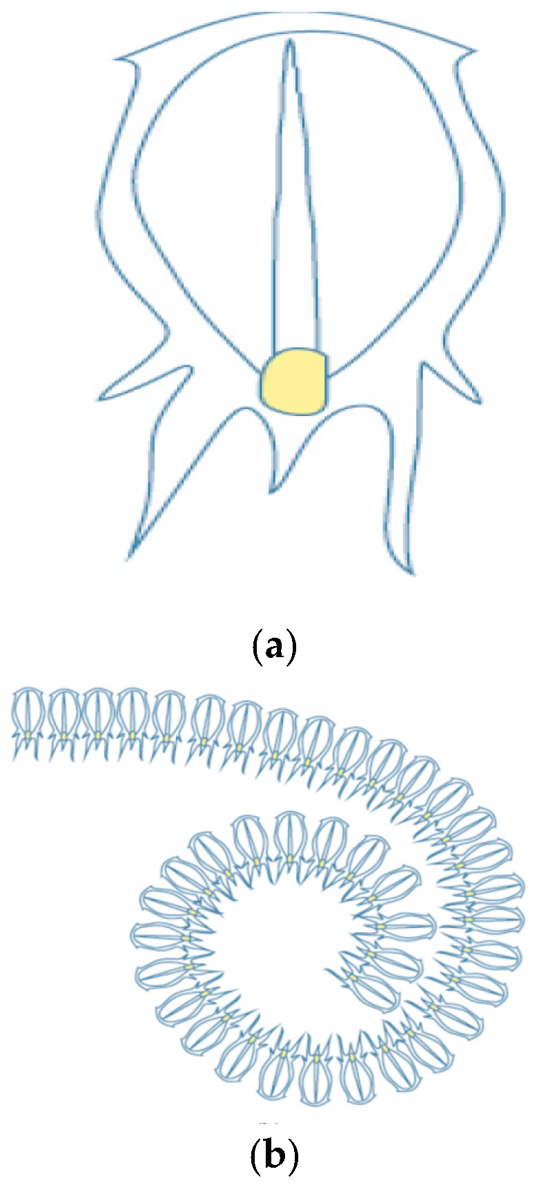
Salps belong to the Salpidae family, with the body structure of a limpid cylinder. They resemble jellyfish in their movement and texture. The Salp’s shape is depicted in
Figure 1a. These creatures follow a special swarm movement. They move forward as a result of the push of the water [
7]. This swarming attitude is the chief inspiration for the development of an algorithm called the Salp Swarm Algorithm [
8]. These Salps form a Salp chain in the oceans, which helps these creatures to attain the best movements in the foraging process. This chain is demonstrated in
Figure 1b.
Mathematical Model
In order to create a mathematical model for the Salp chains, the entire Salp population in a chain is divided into two groups, namely, the head and the followers. The head is the start of the chain, and the remainders of the chain are the followers [
9].
The Salp’s position is defined in a search space of dimension n, where n signifies the number of variables in the problem.
Then, a 2D matrix with the name
x, which reserves the position of each Salp, is defined. There is also an assumed food source as the target of the swarm. The position of a leader is upgraded using the equation
where
xI j is the leader Salp’s position in the jth dimension;
is the food source’s position in the jth dimension;
is the jth dimension’s upper bound;
is the jth dimension’s lower bound;
, , and are random numbers.
From Equation (6), it is clear that the updating of the leader’s position solely depends on the food source.
The coefficient
is a vital parameter in USSA, as it strikes the balance of exploration and exploitation. Hence, it is calculated as
where
The parameters and represent random numbers regularly produced in the interval of [0, 1]. The importance of these parameters is that they determine whether the next position of the leader in the jth dimension should be towards positive or negative infinity. Apart from that, they also determine the step size.
Meanwhile, the updating of the follower’s position is performed using the equation of Newton’s law of motion, which is formulated as
where
Because iteration is the time in optimization, the difference between iterations is 0 and 1, and if
v0 = 0, then the equation can be modified as
where
The Salp chains can be simulated using Equations (6) and (9).
The following section will provide a description of the localization of non-localized nodes in UWSN using the Salp’s algorithm.
3. Node Localization Using Underwater Salp Swarm Optimization Algorithm (USSA)
Despite proposing Salp to solve the localization problem, the study understood that these mathematical models cannot be directly used to find the solution to optimization problems in the underwater environment. Hence, the study modified the algorithm to chase the moving global optimum [
10], which in turn facilitates the localization of all non-localized nodes. The localization procedure is detailed in the subsequent paragraphs.
The USSA approached the global optimum by introducing several Salps with random positions [
11]. Then, it estimated the fitness of every Salp to figure out the Salp with the best fitness. Once this had been determined, the algorithm assigned the best Salp’s position as the source food, represented by variable F, to be searched by the rest of the Salp chain. In the meantime, the coefficient
, which balances the exploration process, was updated using Equation (9). The entire process was iteratively executed until all non-localized nodes were localized.
Key Features of USSA
There are certain key advantages of the USSA, which make the algorithm capable of localizing the nodes. These features are specified below:
- ■
In each iteration, the USSA preserves the best solution achieved thus far and allocates it to the global optimum variable [
12]. This process helps to prevent the loss of the solution, even in the case of the deterioration of whole populations.
- ■
The USSA updates the leading Salp’s position only with reference to the best solution attained so far. This ensures that the leader continuously explores the space around it, which in turn enables the localization [
13] of other non-localized nodes.
- ■
The position of the follower Salps, with reference to one another, has been updated by the algorithm. This helps the followers to gradually approach the leading Salp.
- ■
Further, this gradual movement of follower Salps prevents the stagnation [
14] of the algorithm.
- ■
The adaptive decreasing of parameter c
1, along with the iterations [
15], enables the algorithm to explore the search space first before exploiting it.
- ■
There is only a single major controlling parameter () for the USSA.
4. Performance Comparison and Results
4.1. Simulation Setups and Determination of Performance Parameters
This study conducts a performance comparison of the Underwater SALP Swarm Optimization Algorithm (USSA) with the Underwater Particle Swarm Optimization Algorithm (UPSO), and the Underwater Butterfly Optimization Algorithm (UBOA). The performance parameters, such as the computing time, the number of localized nodes, and the localization error are measured as a part of analyzing the performance of the selected algorithms. MATLAB was used to perform the simulation.
Simulation Settings
The simulation parameters used for the proposed optimization algorithm are depicted in
Table 1.
The anchor nodes are the nodes that already know their location and have the highest energy in the underwater environment.
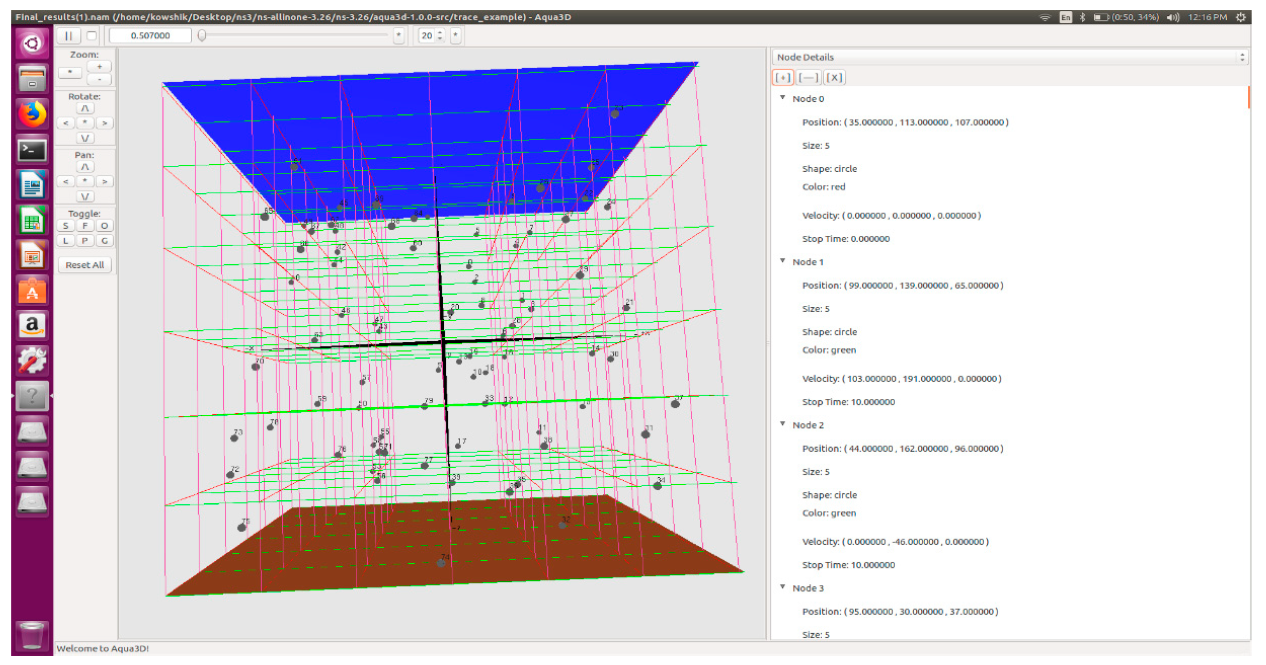
The result addresses the problems during the localization of non-localized nodes in the 3-D underwater environment. The study found out that the determination of the sensor node’s 3-D position coordinates in the real-time aquatic environment is one of the major challenges faced during the localization of nodes, and that a proper visualization tool can help to overcome this difficulty. A sample deployment representation is shown in
Figure 2.
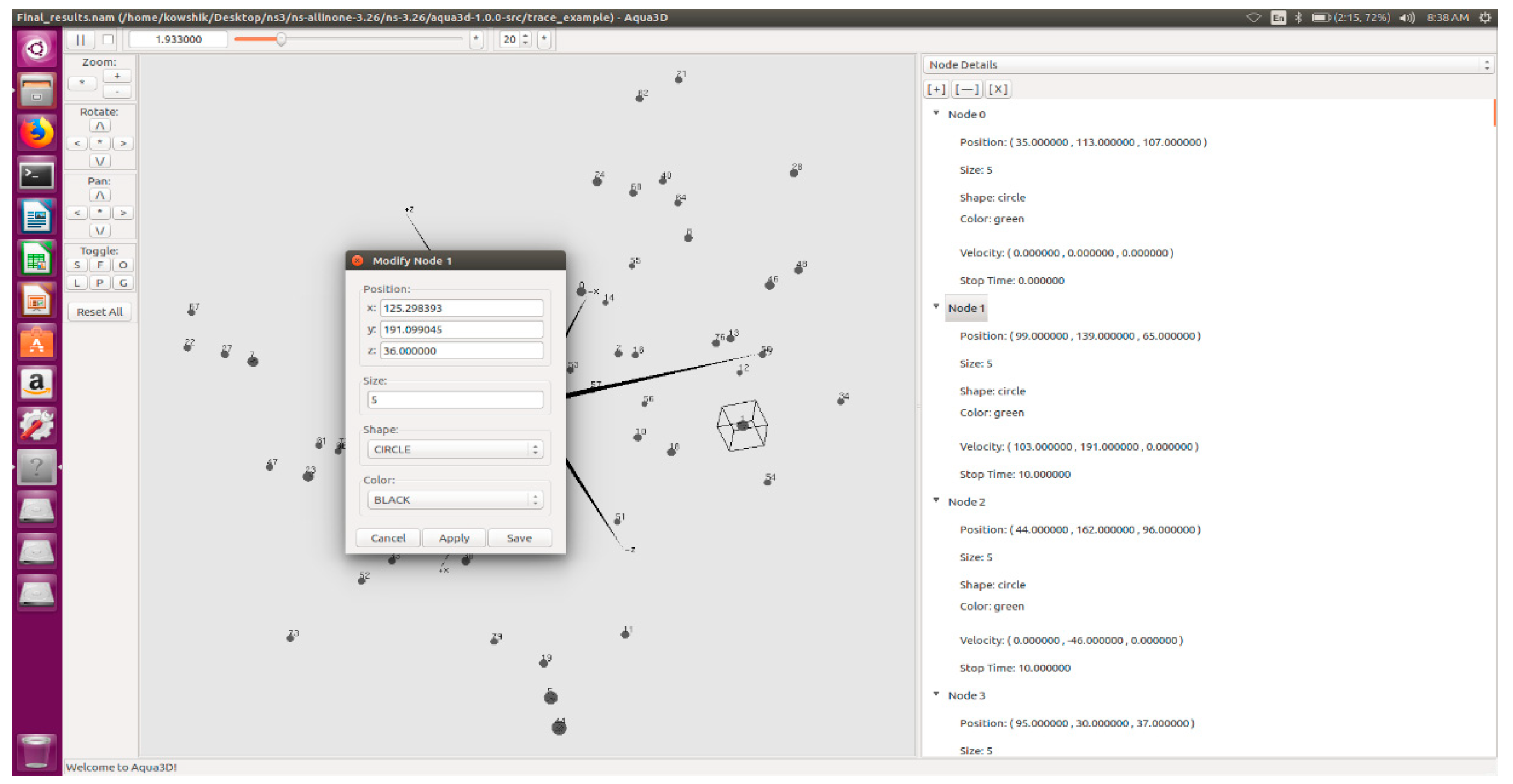
The coordinate values change during the simulation time. The node 1 coordinate values can be observed in
Figure 3.
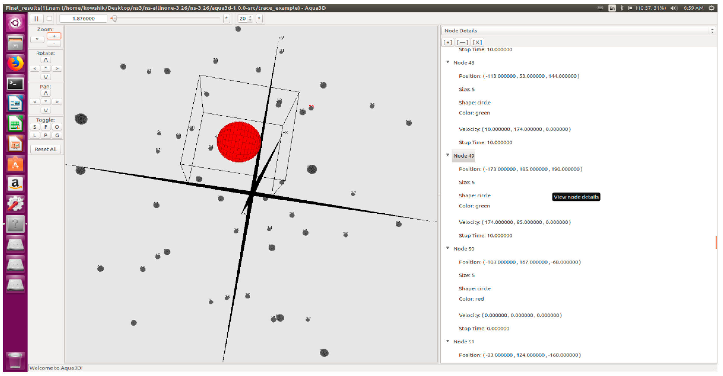
A sample view of node 49, changing with respect to the simulation time, can be observed in
Figure 4. The total simulation time considered is 10 s, and the observation and comparative analysis of the work are carried out for 2 s.
The findings of the comparative analysis are provided in the subsequent section.
4.2. Results
4.2.1. Computing Time
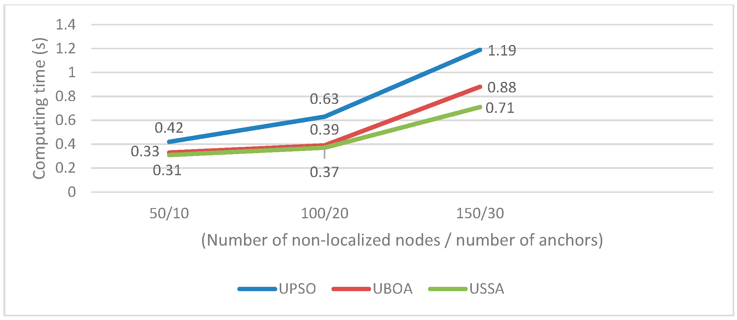
Figure 5 depicts the findings of the comparative analysis of the proposed USSA, UBOA, and UPSO, with respect to the computing time.
It can be inferred from
Figure 5 that the computation time of all the algorithms kept increasing, with reference to the rise in the number of the non-localized nodes and the anchor nodes. However,
Figure 5 makes it clear that the proposed USSA took lesser computing time in comparison with the other two algorithms. This was evident for all the selected non-localized nodes–number of anchor combinations [
16]. Even though the UBOA showcased an almost similar performance in a lesser number of the non-localized nodes and the anchor nodes combination, the gap kept widening as the count of the non-localized nodes and the anchor nodes increased; in the end, it took a computing time of 0.88 s to localize 150 non-localized nodes with the help of 30 anchor nodes, whereas the USSA only took 0.71 s. The comparison of the USSA with the UPSO demonstrated a much wider gap in the computing time, with the UPSO having a much higher computing time compared with the USSA. Hence, the result proves the performance supremacy [
17] of the USSA over the UBOA and the UPSO in the localization of non-localized nodes, with reference to the computing time.
4.2.2. Number of Localized Nodes
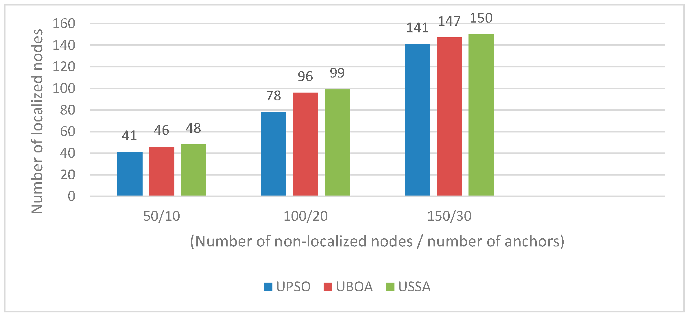
Figure 6 depicts the findings of the comparative analysis of the proposed USSA, UBOA, and UPSO, with reference to the number of localized nodes.
Figure 6 makes it clear that the proposed USSA managed to localize the highest number of non-localized nodes in comparison with the contemporary algorithms. This performance supremacy was evident in different non-localized anchor nodes combinations, even though the UBOA performed very closely. Further, the rise in the number of localized nodes, with reference to the rise in the non-localized node and anchor node density [
18], indicates that the count of localized nodes increases along with the surge in the count of anchor nodes. This also proves the performance efficiency of the proposed USSA.
4.2.3. Localization Error
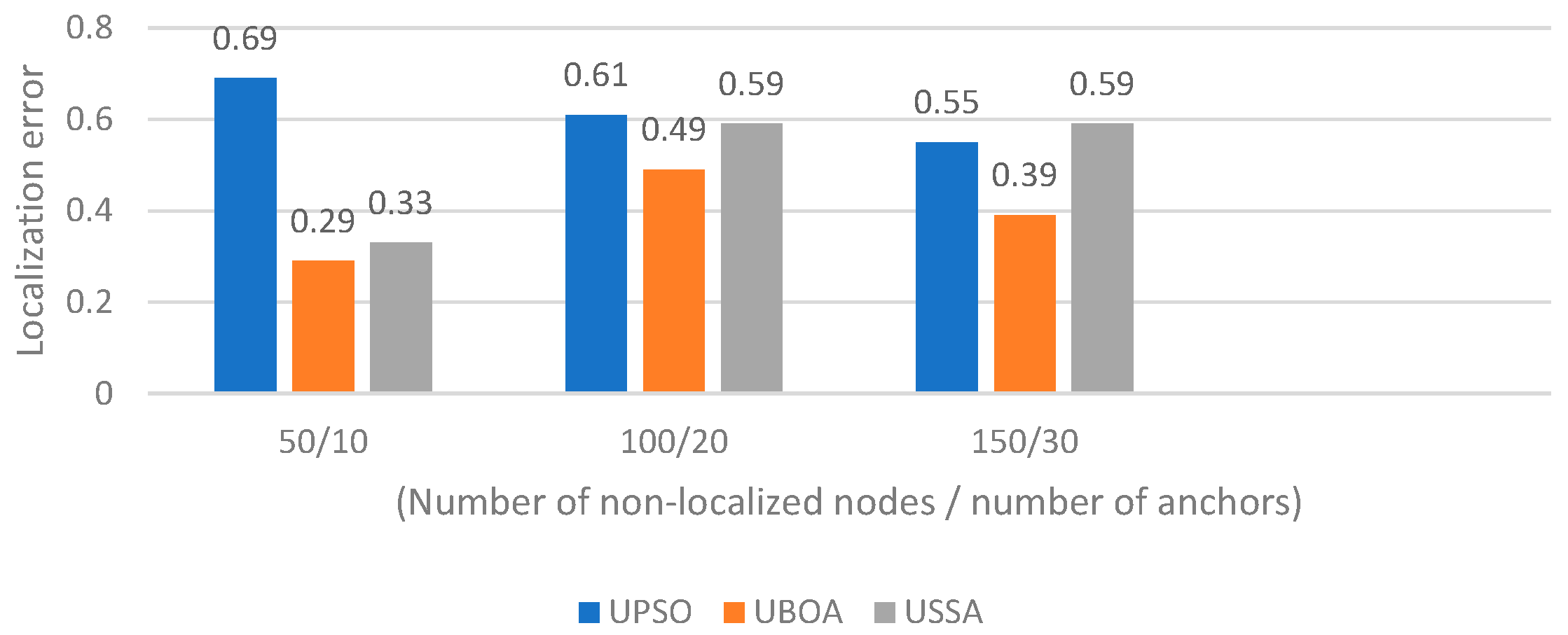
The findings of the comparative analysis of the USSA, UBOA, and UPSO, with respect to the localization error, are depicted in
Figure 7.
The findings, as indicated in
Figure 7, revealed that the UBOA yielded the best output with the least localization error among the three algorithms. The proposed USSA yielded a result close to the best performer UBOA when the count of the anchor and non-localized nodes was less (yielded an output with a localization error of 0.33 for 50 non-localized nodes and 10 anchor nodes). However, the error rate of the proposed USSA increased as the count of the anchor nodes and non-localized nodes increased. Despite this increase, it maintained a constant error value with reference to the upsurge in the number of non-localized nodes and anchor nodes. This result justifies the selection of the USSA to a certain extent, as with these constant error rates, it is possible to localize more number of nodes by increasing the number of anchor nodes [
19]. In addition, the superior performance of the USSA over the UPSO also indicates that the proposed USSA is not an incorrect choice.
4.3. Performance Metrics of Selected Localization Algorithms
The summary of the performance analysis of the selected localization algorithms is described in the subsequent
Table 2 and
Table 3.
Table 2 demonstrated that the rise in the number of iterations causes a corresponding rise in computing time. This was evident with respect to all selected algorithms. The reason is that, as the number of iterations rises, a larger amount of computations is required, which, in turn, leads to a longer computation time. Meanwhile, the localization error, as well as the number of localized nodes, showcased a mixed result with no clear pattern to indicate the relationship of these performance metrics with the number of non-localized nodes, as well as anchor nodes. Further,
Table 2 and
Table 3 also indicated the supreme performance of the suggested USSA with reference to the number of localized nodes and the computing time. This performance supremacy was evident across different iterations and various combinations of non-localized and anchor nodes. In brief,
Table 2 and
Table 3 justify the proposal of the USSA and the iterative procedure.
5. Conclusions
In this paper, a nature-inspired node localization algorithm named the Salp Swarm Algorithm (USSA) has been proposed to tackle the localization problem occurring in the UWSNs. This algorithm handled the localization problem as an optimization problem and attempted to find a solution. The suggested USSA has been implemented in a simulated environment and was validated using various numbers of non-localized and anchor nodes. Furthermore, the suggested algorithm was assessed and compared with other existing optimization algorithms, namely the UPSO and the UBOA, with reference to computing time, localization accuracy, and the number of localized nodes. The simulation results substantiated the performance supremacy of the proposed USSA over the other two localization algorithms with respect to the number of localized nodes and the computing time. Even though the UBOA yielded the best output with the least localization error, the close result yielded by the proposed USSA when the number of anchors and non-localized nodes is less indicated that the USSA was not a bleak performer. Moreover, the constant error value it maintained also justifies the selection of the USSA to a certain extent, as with these constant error rates, it is possible to localize more nodes by raising the number of anchor nodes. In brief, the proposal of the USSA is justified by its performance efficiency.
6. Discussion
A naturally inspired Underwater Salp Swarm Algorithm (USSA) was proposed and the performance was compared with other existing optimization algorithms, namely the UPSO and UBOA, with respect to the computing time, the localization accuracy, and the number of localized nodes. The findings substantiated the performance supremacy of the proposed USSA over the other two localization algorithms [
20], with respect to the parameters, the number of localized nodes, and the computing time. The findings demonstrated that the suggested USSA only took 0.71 s to localize 150 nodes, whereas the UBOA took 0.88 s and the UPSO took 1.19 s. Even though the UBOA yielded the best output with the least localization error among the selected algorithms, the close result yielded by the proposed USSA when the number of non-localized and anchor nodes was lower [
21] (yielding an output with a localization error of 0.33, where the UBOA demonstrated an error rate of 0.29, for 50 non-localized nodes and 10 anchor nodes), indicated that the USSA was not a bleak performer. Moreover, the constant error value it maintained also justifies the selection of the USSA to a certain extent, as with these constant error rates, it is possible to localize a greater number of nodes [
22] by raising the number of anchor nodes.
Author Contributions
Conceptualization, Y.B.H. and Y.N.; methodology, A.B.N. and N.K.C.M.; software, N.K.C.M. and Y.N.; validation, Y.B.H., A.B.N. and Y.N.; formal analysis, N.K.C.M. and Y.N.; investigation, Y.B.H.; resources, N.K.C.M. and Y.N.; data curation, A.B.N.; writing—original draft preparation, Y.N.; writing—review and editing, Y.B.H., A.B.N., N.K.C.M. and Y.N. All authors have read and agreed to the published version of the manuscript.
Funding
This research received no external funding.
Institutional Review Board Statement
Not applicable.
Informed Consent Statement
Not applicable.
Data Availability Statement
Not applicable.
Conflicts of Interest
The authors declare no conflict of interest.
References
- Gopakumar, A.; Jacob, L. Localization in wireless sensor networks using particle swarm optimization. In Proceedings of the IET International Conference on Wireless, Mobile and Multimedia Networks, Beijing, China, 11–12 January 2008; pp. 227–230. [Google Scholar]
- Harikrishnan, R.; Kumar, V.J.S.; Ponmalar, P.S. Firefly algorithm approach for localization in wireless sensor networks. In Proceedings of the 3rd International Conference on Advanced Computing, Networking and Informatics, Bhubaneswar, India, 23–25 June 2015; Springer: Berlin/Heidelberg, Germany, 2016; pp. 209–214. [Google Scholar]
- Fouad, M.M.; Hafez, A.I.; Hassanien, A.E.; Snasel, V. Grey wolves optimizer-based localization approach in wsns. In Proceedings of the 11th International Computer Engineering Conference (ICENCO), Cairo, Egypt, 29–30 December 2015; pp. 256–260. [Google Scholar]
- Arora, S.; Singh, S. Butterfly algorithm with levy flights for global optimization. In Proceedings of the IEEE International Conference in Signal Processing, Computing and Control (ISPCC), Waknaghat, India, 24–26 September 2015; pp. 220–224. [Google Scholar]
- Blair, R.B.; Launer, A.E. Butterfly diversity and human land use: Species assemblages along an urban grandient. Biol. Conserv. 1997, 80, 113–125. [Google Scholar] [CrossRef]
- Eberhart, R.; Kennedy, J. Particle swarm optimization. In Proceedings of the IEEE International Conference on Neural Networks, Perth, Australia, 27 November–1 December 1995; Volume 4, pp. 1942–1948. [Google Scholar]
- Madin, L.P. Aspects of jet propulsion in Salps. Can. J. Zool. 1990, 68, 765–777. [Google Scholar] [CrossRef]
- Mirjalili, S.; Gandomi, A.H.; Mirjalili, S.Z.; Saremi, S.; Faris, H.; Mirjalili, S.M. Salp swarm algorithm: A bio-inspired optimizer for engineering design problems. Adv. Eng. Softw. 2017, 114, 163–191. [Google Scholar] [CrossRef]
- Ibrahim, H.T.; Mazher, W.J.; Ucan, O.N.; Bayat, O. Feature selection using salp swarm algorithm for real biomedical datasets. Int. J. Comput. Sci. Netw. Secur. 2017, 17, 13–20. [Google Scholar]
- Arora, S.; Singh, S. Node localization in wireless sensor networks using butterfly optimization algorithm. Arab. J. Sci. Eng. 2017, 42, 3325–3335. [Google Scholar] [CrossRef]
- Anuradha, D.; Subramani, N.; Khalaf, O.I.; Alotaibi, Y.; Alghamdi, S.; Rajagopal, M. Chaotic Search-and-Rescue-Optimization-Based Multi-Hop Data Transmission Protocol for Underwater Wireless Sensor Networks. Sensors 2022, 22, 2867. [Google Scholar] [CrossRef] [PubMed]
- Lalama, Z.; Boulfekhar, S.; Semechedine, F. Localization Optimization in WSNs Using Meta-Heuristics Optimization Algorithms: A Survey. Wirel. Pers. Commun. 2022, 122, 1197–1220. [Google Scholar] [CrossRef]
- Alotaibi, Y. A New Meta-Heuristics Data Clustering Algorithm Based on Tabu Search and Adaptive Search Memory. Symmetry 2022, 14, 623. [Google Scholar] [CrossRef]
- Gou, P.; He, B.; Yu, Z. A Node Location Algorithm Based on Improved Whale Optimization in Wireless Sensor Networks. Wirel. Commun. Mob. Comput. 2021, 2021, 7523938. [Google Scholar] [CrossRef]
- Mohan, P.; Subramani, N.; Alotaibi, Y.; Alghamdi, S.; Khalaf, O.I.; Ulaganathan, S. Improved metaheuristics-based clustering with multihop routing protocol for underwater wireless sensor networks. Sensors 2022, 22, 1618. [Google Scholar] [CrossRef] [PubMed]
- Fé, J.; Correia, S.D.; Tomic, S.; Beko, M. Swarm optimization for energy-based acoustic source localization: A comprehensive study. Sensors 2022, 22, 1894. [Google Scholar] [CrossRef] [PubMed]
- Subramani, N.; Mohan, P.; Alotaibi, Y.; Alghamdi, S.; Khalaf, O.I. An efficient metaheuristic-based clustering with routing protocol for underwater wireless sensor networks. Sensors 2022, 22, 415. [Google Scholar] [CrossRef] [PubMed]
- Bharany, S.; Sharma, S.; Badotra, S.; Khalaf, O.I.; Alotaibi, Y.; Alghamdi, S.; Alassery, F. Energy-efficient clustering scheme for flying ad-hoc networks using an optimized LEACH protocol. Energies 2021, 14, 6016. [Google Scholar] [CrossRef]
- Song, J.; Jin, H.; Shen, X.; Zhang, S. A Maximum Localization Rate Algorithm for 3D Large-Scale UWSNs. IEEE Access 2022, 10, 111962–111973. [Google Scholar] [CrossRef]
- Li, Y.; Liu, M.; Zhang, S.; Zheng, R.; Lan, J.; Dong, S. Particle System-Based Ordinary Nodes Localization With Delay Compensation in UWSNs. IEEE Sens. J. 2022, 22, 7157–7168. [Google Scholar] [CrossRef]
- Sivakumar, V.; Rekha, D. Node scheduling problem in underwater acoustic sensor network using genetic algorithm. Pers Ubiquit Comput 2018, 22, 951–959. [Google Scholar] [CrossRef]
- Sivakumar, V.; Rekha, D. A QoS-aware energy-efficient memetic flower pollination routing protocol for underwater acoustic sensor network. Concurrency Computat Pract Exper. 2020, 32, e5166. [Google Scholar] [CrossRef]
| Publisher’s Note: MDPI stays neutral with regard to jurisdictional claims in published maps and institutional affiliations. |
© 2022 by the authors. Licensee MDPI, Basel, Switzerland. This article is an open access article distributed under the terms and conditions of the Creative Commons Attribution (CC BY) license (https://creativecommons.org/licenses/by/4.0/).

 ,
, 


