Geometric Interpretation and General Classification of Three-Dimensional Polarization States through the Intrinsic Stokes Parameters


Abstract
:1. Introduction
2. Materials and Methods
3. Results
3.1. The Polarization Object
3.2. Classification of Three-Dimensional Polarization States Based on the Polarization Object

| (2D states) | ||||
| (pure states) | (2D mixed states) | |||
| Linear | Elliptical | Circular | Partially polarized | Unpolarized |
| Indep. parameters: | Indep. parameters: | Indep. parameters: | Indep. parameters: | Indep. parameters: |
| Principal variances: | Principal variances: | Principal variances: | Principal variances: | Principal variances: |
| Spin density vector: | Spin density vector: | Spin density vector: | Spin density vector: | Spin density vector: |
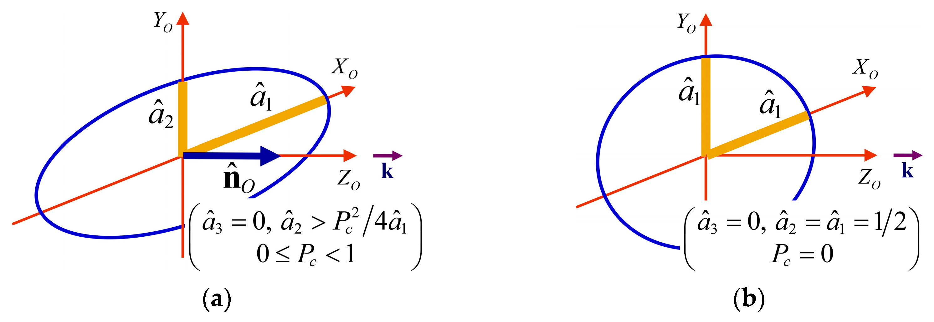
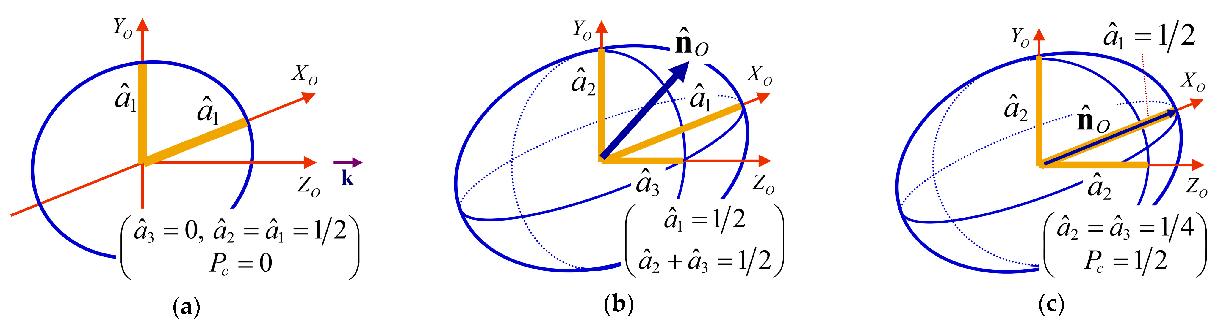
| Polarization object: Figure 2a | Polarization object: Figure 2b | Polarization object: Figure 2c | Polarization object: Figure 3a | Polarization object: Figure 3b |
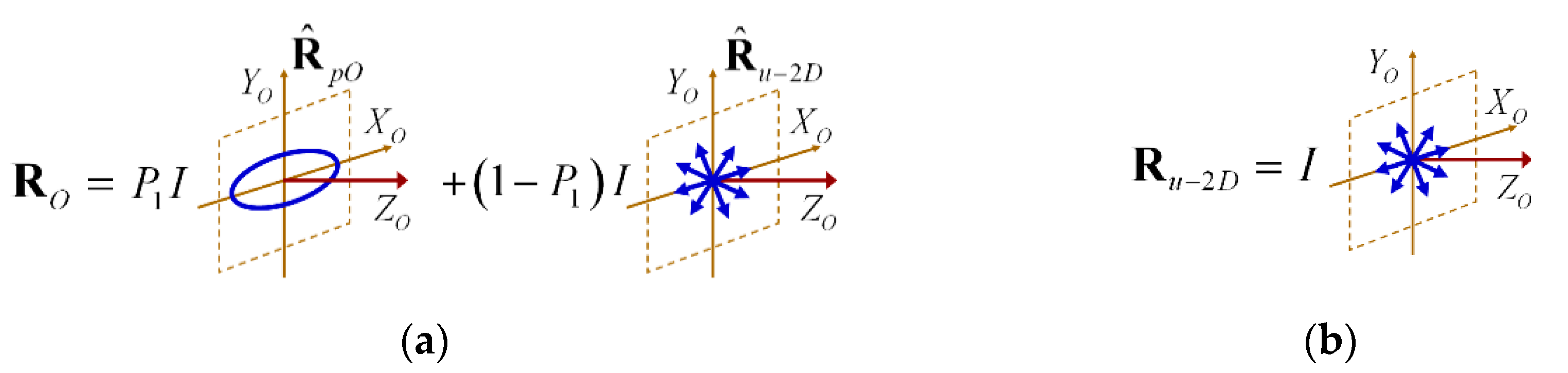
| Characteristic decomposition: | Characteristic decomp.: Figure 4a | Characteristic decomp.: Figure 4b | ||
| (genuine 3D states) | |
| Regular 3D mixed states | Nonregular 3D mixed states |
| Independent parameters: | Independent parameters: |
| Principal variances: | Principal variances: |
| Spin density vector: | Spin density vector: |
| Polarization object: Figure 5a | Polarization object: Figure 5b |
| Characteristic decomposition: Figure 6 | Characteristic decomposition: Figure 7 |
| (discriminating states, ) | ||
| 2D unpolarized state | Nonregular discriminating state | Perfect nonregular state |
| Independent parameters: | Independent parameters: | Independent parameters: |
| Principal variances: | Principal variances: | Principal variances: |
| Spin density vector: | Spin density vector: | Spin density vector: |
| Polarization object: Figure 8a | Polarization object: Figure 8b | Polarization object: Figure 8c |
4. Discussion
- ⇔ R is a 2D state ⇔ the polarization density ellipsoid is an ellipse.
- ○
- ⇔ R is a 2D mixed state.
- ▪
- ⇔ R is a 2D unpolarized state (i.e., R is a 2D discriminating state), ( and ).
- ○
- ⇔ R is a pure state, .
- ▪
- ⇔ R is a linearly polarized pure state, .
- ▪
- ⇔ R is an elliptically polarized pure state, , with .
- ▪
- ⇔ R is a circularly polarized pure state, with .
- ⇔ R is a genuine 3D state.
- ○
- or ⇔ R is a regular genuine 3D state.
- ○
- and not parallel to ⇔ R is a nonregular state.
- ○
- ⇔ The polarization density ellipsoid E of R is a sphere (, full intensity isotropy, )
- ▪
- ⇔ (full intensity isotropy, , with nonzero spin).
- ▪
- ⇔ R is a 3D unpolarized state, (full intensity and spin isotropy).
- ○
- ⇔ R is a 3D discriminating state, (, and not parallel to ).
- ▪
- ⇔ R is a perfect nonregular state
5. Conclusions
Funding
Informed Consent Statement
Conflicts of Interest
Appendix A
| Structure or Quantity | Definition | Properties | Physical Meaning |
|---|---|---|---|
| Intensity | Invariant under rotation and under the action of birefringent devices | Averaged power of the electromagnetic wave at point r | |
| Polarization matrix | R | Hermitian positive semidefinite | Provides complete information on second-order polarization properties |
| Polarization density matrix | Hermitian positive semidefinite, with | Intensity-normalized polarization matrix. Formally equivalent to a density matrix | |
| Eigenvalues of | Relative weights of the spectral incoherent components of [20] | ||
| Indices of polarimetric purity (IPP) | The IPP provide a complete quantitative characterization of the structure of polarimetric purity [36,37] | ||
| Intrinsic polarization matrix | Intrinsic representation of the polarization state. Principal variances: Spin density vector: | Represents the same state as R, but referenced with respect to the corresponding intrinsic reference frame. The off-diagonal elements are pure imaginary because is defined through the diagonalization of the real part of R [20,33]. | |
| Principal variances of | Semiaxes of the polarization density ellipsoid [20,33]. | ||
| Spin vector | Spin vector of the state, with dimensions of intensity [33,47] | ||
| Spin density vector | Spin density vector of the state (nondimensional) [20,33] | ||
| Spin density | Absolute value of the spin density vector. Is a measure of the degree of circular polarization of the state | ||
| Polarization object | Intensity ellipsoid , with semiaxes and spin vector | Rigid composition of and The orientation angles of with respect to the symmetry axes XOYOZO of are fixed and invariant | Determines geometrically all intrinsic properties of the state. |
| Polarization density object | polarization density ellipsoid E, with semiaxes and spin density vector | Rigid composition of E and The orientation angles of with respect to the symmetry axes XOYOZO of are fixed and invariant | Determines geometrically all intrinsic properties of the state, but I, as with the Poincaré sphere of 2D polarization states |
| Orientation angles of the polarization object | determine the rotation from the intrinsic reference frame axes XOYOZO to an arbitrary one. | The angles that allow for representing the polarization object with respect to a given reference frame | |
| Degree of linear polarization | An objective measure of how close to a linearly polarized state the state is [20,21] | ||
| Degree of circular polarization | An objective of how close to a circularly polarized state the state is [20,21] | ||
| Degree of directionality | An objective measure of the degree of stability of the plane containing the fluctuating polarization ellipse. Equivalently, a measure of the closeness of the 3D state to a 2D one [20,21] | ||
| Intrinsic Stokes parameters | Intrinsic measurable quantities. Have phenomenological nature: They are always well defined, regardless of the underlying microscopic model considered [20,21] | ||
| Dimensionality index, d and polarimetric dimension, . | Determine the effective dimensions taking place in the state. : linearly polarized; , 2D state; , 3D state [41] | ||
| Degree of polarimetric purity | An objective measure of how close to a pure state R is. It is determined by: (1) IPP contributions; (2) CP contributions and (3) Intensity and spin anisotropies [38,43] | ||
| Complete parameterization of R | Determine completely the polarization object and its spatial orientation with respect to the laboratory reference frame | Complete information carried by R in terms of nine meaningful quantities: the six intrinsic Stokes parameters and the three orientation angles of the polarization density object [20,21] | |
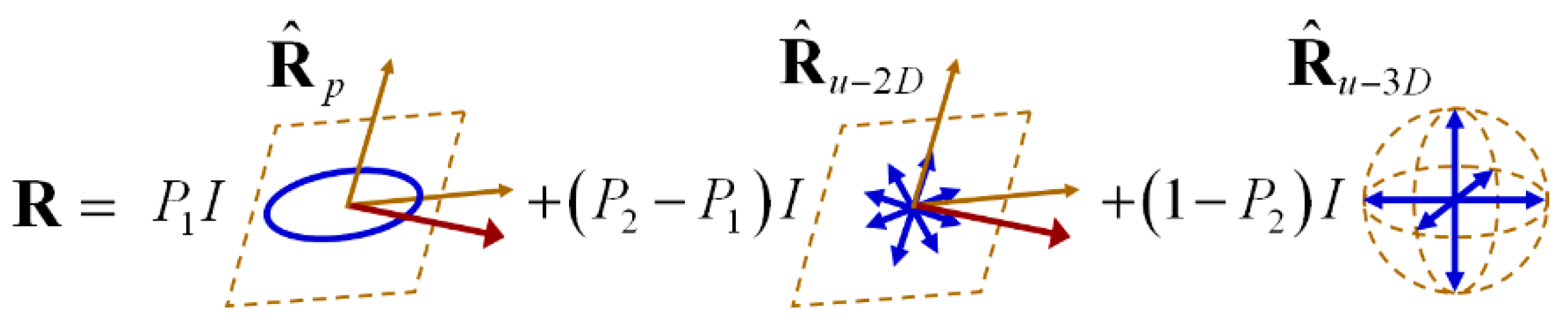
| Characteristic decomposition | R is polarimetrically equivalent to an incoherent composition of pure state , a discriminating state and a unpolarized state | In the case of 2D states becomes the well known decomposition into an incoherent combination of a pure state and a 2D unpolarized state [39] | |
| Discriminating component (in its own intrinsic representation) | This is the general form of a discriminating state, when referenced with respect to its own intrinsic reference frame [42] | In general, the discriminating component is different from . When , then is a 3D state and is said to be nonregular Nonregular discriminating states exhibit nonzero spin, nonzero degree of linear polarization [42] | |
| Degree of nonregularity | An objective measure of the distance of the state to a regular state [42] |
References
- Poincaré, H. Théorie Mathématique de la Lumière; Carre, G., Ed.; Mallet-Bachelier: Paris, France, 1892. [Google Scholar]
- Stokes, G.G. On the composition and resolution o streams of polarized light from different sources. Trans. Cambridge Phil. Soc. 1852, 9, 399–416. [Google Scholar]
- Wiener, N. Coherency matrices and quantum theory. J. Math. Phys. 1928, 7, 109–125. [Google Scholar] [CrossRef]
- Soleillet, P. Sur les paramètres caractérisant la polarisation partielle de la lumière dans les phénomènes de fluorescence. Ann. Phys. 1929, 10, 23–97. [Google Scholar] [CrossRef]
- Falkoff, D.L.; Macdonald, J.E. On the Stokes Parameters for Polarized Radiation. J. Opt. Soc. Am. 1951, 41, 861–862. [Google Scholar] [CrossRef]
- Fano, U. A Stokes-Parameter Technique for the Treatment of Polarization in Quantum Mechanics. Phys. Rev. 1954, 93, 121–123. [Google Scholar] [CrossRef]
- Wolf, E. Optics in terms of observable quantities. Il Nuovo Cimento B 1954, 12, 884–888. [Google Scholar] [CrossRef]
- Wolf, E. Coherence properties of partially polarized electromagnetic radiation. Il Nuovo Cimento B 1959, 13, 1165–1181. [Google Scholar] [CrossRef]
- Roman, P. Generalized stokes parameters for waves with arbitrary form. Il Nuovo Cimento B 1959, 13, 974–982. [Google Scholar] [CrossRef]
- Samson, J.C. Descriptions of the Polarization States of Vector Processes: Applications to ULF Magnetic Fields. Geophys. J. Int. 1973, 34, 403–419. [Google Scholar] [CrossRef] [Green Version]
- Barakat, R. Degree of polarization and the principal idempotents of the coherency matrix. Opt. Commun. 1977, 23, 147–150. [Google Scholar] [CrossRef]
- Carozzi, T.; Karlsson, R.; Bergman, J. Parameters characterizing electromagnetic wave polarization. Phys. Rev. E 2000, 61, 2024–2028. [Google Scholar] [CrossRef] [Green Version]
- Setälä, T.; Shevchenko, A.; Kaivola, M.; Friberg, A.T. Degree of polarization for optical near fields. Phys. Rev. E 2002, 66, 016615. [Google Scholar] [CrossRef] [Green Version]
- Luis, A. Quantum polarization for three-dimensional fields via Stokes operators. Phys. Rev. A 2005, 71. [Google Scholar] [CrossRef] [Green Version]
- Korotkova, O.; Wolf, E. Generalized Stokes parameters of random electromagnetic beams. Opt. Lett. 2005, 30, 198–200. [Google Scholar] [CrossRef]
- Petrov, N.I. Vector and tensor polarizations of light beams. Laser Phys. 2008, 18, 522–525. [Google Scholar] [CrossRef]
- Sheppard, C.J.R. Partial polarization in three dimensions. J. Opt. Soc. Am. A 2011, 28, 2655–2659. [Google Scholar] [CrossRef]
- Sheppard, C.J.R. Geometric representation for partial polarization in three dimensions. Opt. Lett. 2012, 37, 2772–2774. [Google Scholar] [CrossRef]
- Sheppard, C.J.R. Jones and Stokes parameters for polarization in three dimensions. Phys. Rev. A 2014, 90. [Google Scholar] [CrossRef]
- Gil, J.J. Interpretation of the coherency matrix for three-dimensional polarization states. Phys. Rev. A 2014, 90, 043858-11. [Google Scholar] [CrossRef] [Green Version]
- Gil, J.J. Intrinsic Stokes parameters for 2D and 3D polarization states. J. Eur. Opt. Soc. Rapid. Publ. 2015, 10, 15054–15055. [Google Scholar] [CrossRef] [Green Version]
- Sheppard, C.J.R.; Bendandi, A.; Le Gratiet, A.; Diaspro, A. Eigenvectors of polarization coherency matrices. J. Opt. Soc. Am. A 2020, 37, 1143. [Google Scholar] [CrossRef]
- Arteaga, O.; Nichols, S. Soleillet’s formalism of coherence and partial polarization in 2D and 3D: Application to fluorescence polarimetry. J. Opt. Soc. Am. A 2018, 35, 1254–1260. [Google Scholar] [CrossRef]
- Williams, M.W. Depolarization and cross polarization in ellipsometry of rough surfaces. Appl. Opt. 1986, 25, 3616–3622. [Google Scholar] [CrossRef]
- Le Roy-Brehonnet, F.; Le Jeune, B. Utilization of Mueller matrix formalism to obtain optical targets depolarization and polarization properties. Prog. Quantum Electron. 1997, 21, 109–151. [Google Scholar] [CrossRef]
- Le Roy-Bréhonnet, F.; Le Jeune, B.; Gerligand, P.Y.; Cariou, J.; Lotrian, J. Analysis of depolarizing optical targets by Mueller matrix formalism. Pure Appl. Opt. J. Eur. Opt. Soc. Part A 1997, 6, 385–404. [Google Scholar] [CrossRef]
- Brosseau, C. Fundamentals of Polarized Light: A Statistical Optics Approach; Wiley: Hoboken, NJ, USA, 1998. [Google Scholar]
- Lu, S.-Y.; Chipman, R.A. Mueller matrices and the degree of polarization. Opt. Commun. 1998, 146, 11–14. [Google Scholar] [CrossRef]
- Deboo, B.; Sasian, J.; Chipman, R. Degree of polarization surfaces and maps for analysis of depolarization. Opt. Express 2004, 12, 4941–4958. [Google Scholar] [CrossRef]
- Ferreira, C.; Gil, J.J.; Correas, J.M.; San José, I. Geometric modeling of polarimetric transformations. Monog. Sem. Mat. G. Galdeano 2006, 33, 115–119. [Google Scholar]
- Tudor, T.; Manea, V. Ellipsoid of the polarization degree: A vectorial, pure operatorial Pauli algebraic approach. J. Opt. Soc. Am. B 2011, 28, 596–601. [Google Scholar] [CrossRef]
- Ossikovski, R.; Gil Pérez, J.J.; José, I.S. Poincaré sphere mapping by Mueller matrices. J. Opt. Soc. Am. A 2013, 30, 2291. [Google Scholar] [CrossRef] [PubMed]
- Dennis, M.R. Geometric interpretation of the three-dimensional coherence matrix for nonparaxial polarization. J. Opt. A Pure Appl. Opt. 2004, 6, S26–S31. [Google Scholar] [CrossRef]
- Gil, J.J. Polarimetric characterization of light and media. Eur. Phys. J. Appl. Phys. 2007, 40, 1–47. [Google Scholar] [CrossRef]
- Gil, J.J.; José, I.S. 3D polarimetric purity. Opt. Commun. 2010, 283, 4430–4434. [Google Scholar] [CrossRef]
- Gil, J.J.; Correas, J.M.; Melero, P.A.; Ferreira, C. Generalized polarization algebra. Monog. Sem. Mat. G. Galdeano 2004, 31, 161–167. [Google Scholar]
- San José, I.; Gil, J.J. Invariant indices of polarimetric purity. Generalized indices of purity for nxn covariance matrices. Opt. Commun. 2011, 284, 38–47. [Google Scholar] [CrossRef] [Green Version]
- Gil, J.J. Components of purity of a three-dimensional polarization state. J. Opt. Soc. Am. A 2016, 33, 40–43. [Google Scholar] [CrossRef] [PubMed]
- Gil, J.J.; Friberg, A.T.; Setälä, T. Structure of polarimetric purity of three-dimensional polarization states. Phys. Rev. A 2017, 95, 053856. [Google Scholar] [CrossRef] [Green Version]
- Gil, J.J.; Norrman, A.; Friberg, A.T.; Setälä, T. Polarimetric purity and the concept of degree of polarization. Phys. Rev. A 2018, 97, 023838. [Google Scholar] [CrossRef] [Green Version]
- Norrman, A.; Friberg, A.T.; Gil, J.J.; Setälä, T. Dimensionality of random light fields. J. Eur. Opt. Soc. Rapid Publ. 2017, 13, 1–5. [Google Scholar] [CrossRef] [Green Version]
- Gil, J.J.; Norrman, A.; Friberg, A.T.; Setälä, T. Nonregularity of three-dimensional polarization states. Opt. Lett. 2018, 43, 4611–4614. [Google Scholar] [CrossRef]
- Gil, J.J.; Norrman, A.; Friberg, A.T.; Setälä, T. Intensity and spin anisotropy of three-dimensional polarization states. Opt. Lett. 2019, 44, 3578–3581. [Google Scholar] [CrossRef] [PubMed]
- Gil, J.J.; San José, I.; Norrman, A.; Friberg, A.T.; Setälä, T. Sets of orthogonal three-dimensional polarization states and their physical interpretation. Phys. Rev. A 2019, 100, 033824. [Google Scholar] [CrossRef] [Green Version]
- Gil, J.J. Sources of Asymmetry and the Concept of Nonregularity of n-Dimensional Density Matrices. Symmetry 2020, 12, 1002. [Google Scholar] [CrossRef]
- Gil, J.J.; Ossikovski, R. Polarized Light and the Mueller Matrix Approach; CRC Press: Boca Raton, FL, USA, 2016. [Google Scholar]
- Gil, J.J.; Norrman, A.; Friberg, A.T.; Setälä, T. Effect of polarimetric nonregularity on the spin of three-dimensional polarization states. New J. Phys. 2021, 23, 063059. [Google Scholar] [CrossRef]
- Norrman, A.; Gil, J.J.; Friberg, A.T.; Setälä, T. Polarimetric nonregularity of evanescent waves. Opt. Lett. 2019, 44, 215–218. [Google Scholar] [CrossRef]
- Chen, Y.; Wang, F.; Dong, Z.; Cai, Y.; Norrman, A.; Gil, J.J.; Friberg, A.T.; Setälä, T. Structure of transverse spin in focused random light. Phys. Rev. A 2021, 104, 013516. [Google Scholar] [CrossRef]


Publisher’s Note: MDPI stays neutral with regard to jurisdictional claims in published maps and institutional affiliations. |
© 2021 by the author. Licensee MDPI, Basel, Switzerland. This article is an open access article distributed under the terms and conditions of the Creative Commons Attribution (CC BY) license (https://creativecommons.org/licenses/by/4.0/).
Share and Cite
Gil, J.J. Geometric Interpretation and General Classification of Three-Dimensional Polarization States through the Intrinsic Stokes Parameters. Photonics 2021, 8, 315. https://doi.org/10.3390/photonics8080315
Gil JJ. Geometric Interpretation and General Classification of Three-Dimensional Polarization States through the Intrinsic Stokes Parameters. Photonics. 2021; 8(8):315. https://doi.org/10.3390/photonics8080315
Chicago/Turabian StyleGil, José J. 2021. "Geometric Interpretation and General Classification of Three-Dimensional Polarization States through the Intrinsic Stokes Parameters" Photonics 8, no. 8: 315. https://doi.org/10.3390/photonics8080315