Article

Improving Multiphoton Microscopy by Combining Spherical Aberration Patterns and Variable Axicons

Laboratorio de Óptica, Instituto Universitario de Investigación en Óptica y Nanofísica, Universidad de Murcia, Campus de Espinardo (Ed. 34), 30100 Murcia, Spain
*
Author to whom correspondence should be addressed.
Photonics 2021, 8(12), 573; https://doi.org/10.3390/photonics8120573
Submission received: 11 November 2021 / Revised: 25 November 2021 / Accepted: 9 December 2021 / Published: 13 December 2021
(This article belongs to the Special Issue Laser Interaction with Materials)

Abstract

:
Multiphoton (MP) microscopy is a well-established method for the non-invasive imaging of biological tissues. However, its optical sectioning capabilities are reduced due to specimen-induced aberrations. Both the manipulation of spherical aberration (SA) and the use of axicons have been reported to be useful techniques to bypass this limitation. We propose the combination of SA patterns and variable axicons to further improve the quality of MP microscopy images. This approach provides enhanced images at different depth locations whose quality is better than those corresponding to the use of SA or axicons separately. Thus, the procedure proposed herein facilitates the visualization of details and increases the depth observable at high resolution.

1. Introduction

Multiphoton (MP) microscopy techniques (two-photon excitation fluorescence, TPEF, and second harmonic generation, SHG) combine inherent confocality and minimized tissue damage [1,2]. However, the penetration depth is limited in thick samples mainly due to specimens’ aberrations [3,4]. To overcome this loss of MP effectiveness, different adaptive optics configurations have been used [3,4,5,6].
Among all the aberration terms appearing in thick samples, spherical aberration (SA) is the dominant one [3,5,6,7]. The correction (or minimization) of this SA by using either objective correction collars [8,9] or adaptive optics [3,4,5,6,7,10] has been reported to improve the quality of MP images at deeper locations within the sample. In addition, the manipulation of the SA pattern of the incident beam while performing fast tomographic MP imaging is able to extend the imaging depth [7]. Phase masks [11] and refractive axicons [12,13,14] have also been reported to increase the depth-of-field in MP imaging microscopy without compromising lateral resolution.
A refractive axicon is a conical lens able to transform a Gaussian beam into a non-diffracting Bessel beam [15], which is characterized by both the refractive index and the apex angle of the axicon. These axicons produce an axially elongated focus with a fixed axial length [12,13]. However, when using real-life biological samples, it is often desirable to have Bessel foci of different axial lengths to investigate thick volumes. Different approaches have been reported to adjust this length [14,16]; however, they all require additional optical elements and/or moving parts, which might enlarge the size of the experimental system and complicate its design.
To improve the versatility of Bessel beams, computer-generated holograms and variable diffractive optics elements have been proposed [17,18,19]. In particular, spatial light modulators (SLM) provide a flexible and dynamic way of creating variable non-diffracting beams that can be changed in time [19,20,21,22,23]. This has been implemented into MP microscopes to obtain higher axial resolution and improved penetration depth [24,25,26].
Although the combination of MP imaging and axicons has been successfully demonstrated at deep locations, to our knowledge, the possible detrimental effects of SA within those specimens were not taken into account. In that sense, in this work, we explore the impact of both SA patterns and variable Bessel beams on MP imaging. Since the different Bessel beams are produced by an SLM, they will be referred to as “variable axicons”. An analysis of the feasibility and benefit of using this combination of phase profiles in MP images is carried out here.

2. Materials and Methods

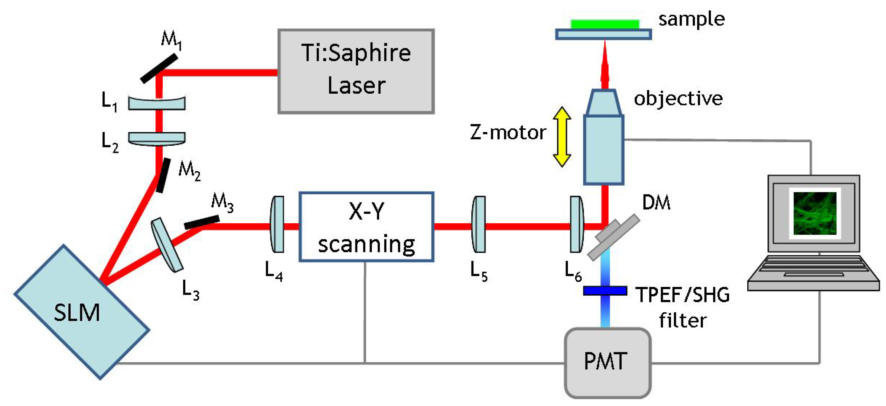
2.1. Experimental Setup

An SLM (Pluto IR2; Holoeye) was incorporated into the illumination pathway of a custom MP microscope. This device was used to project SA and variable axicon phase patterns, both individually and in combination. A schematic diagram of the MP microscope is depicted in Figure 1. The system combines an inverted microscope (Nikon TE2000-U) and a Ti:sapphire laser (Mira900; Coherent) with a central wavelength of 800 nm. The collimated infrared incoming beam was spatially modulated by the SLM and passed the long working-distance non-immersion microscope objective (Nikon ELWD Series, 20×, 0.5 NA). A pair of galvanometric mirrors (VM1000; GSI) served as X-Y scanning unit. A dichroic mirror (DM) separated the (infrared) excitation light from the (visible) nonlinear signal emitted by the sample. A photo-multiplier tube (PMT, R7205-01; Hamamatsu) was used to collect these nonlinear emissions in the backscattered direction. Suitable spectral filters placed in front of the PMT were used to isolate MP signals (either TPEF or SHG) before reaching the PMT. More details on both the instrument and the SLM specifications and functioning can be found elsewhere [6,27]. Moreover, a Z-axis step motor (PI C-136) attached to the objective allowed collecting both X and Y images at different depth locations within the samples. The system was automated and controlled through a custom LabViewTM interface. Image processing was performed with MatLabTM.

2.2. Imaging Protocol
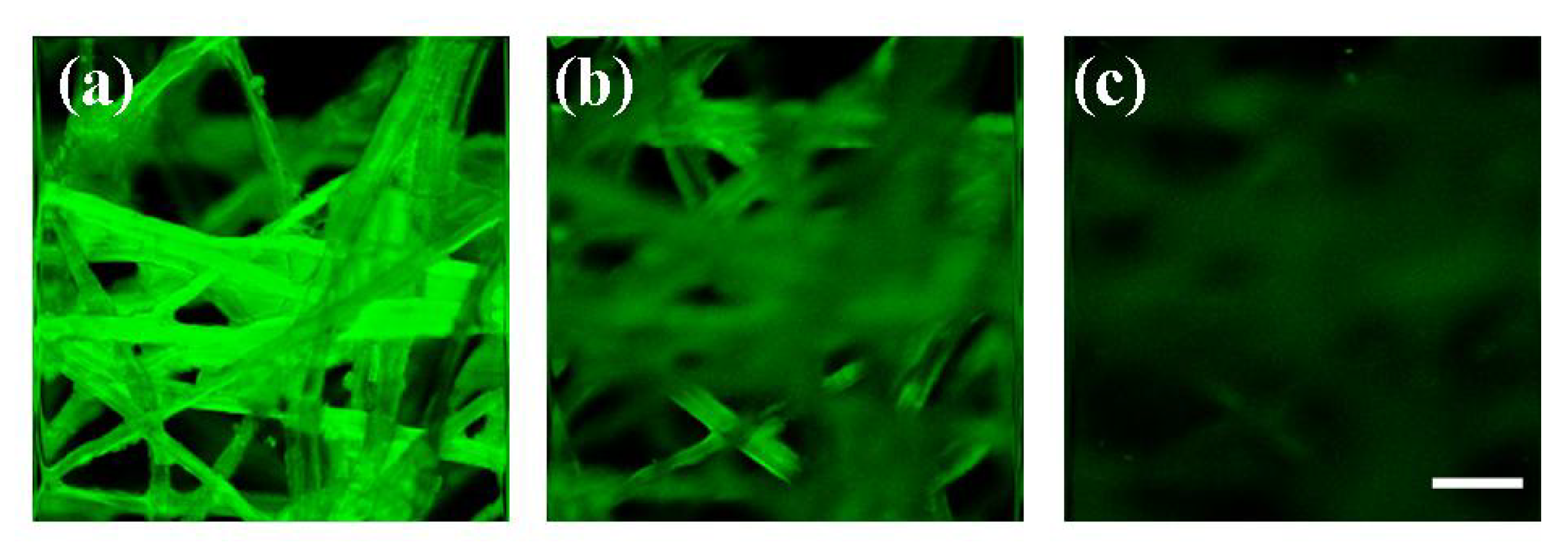
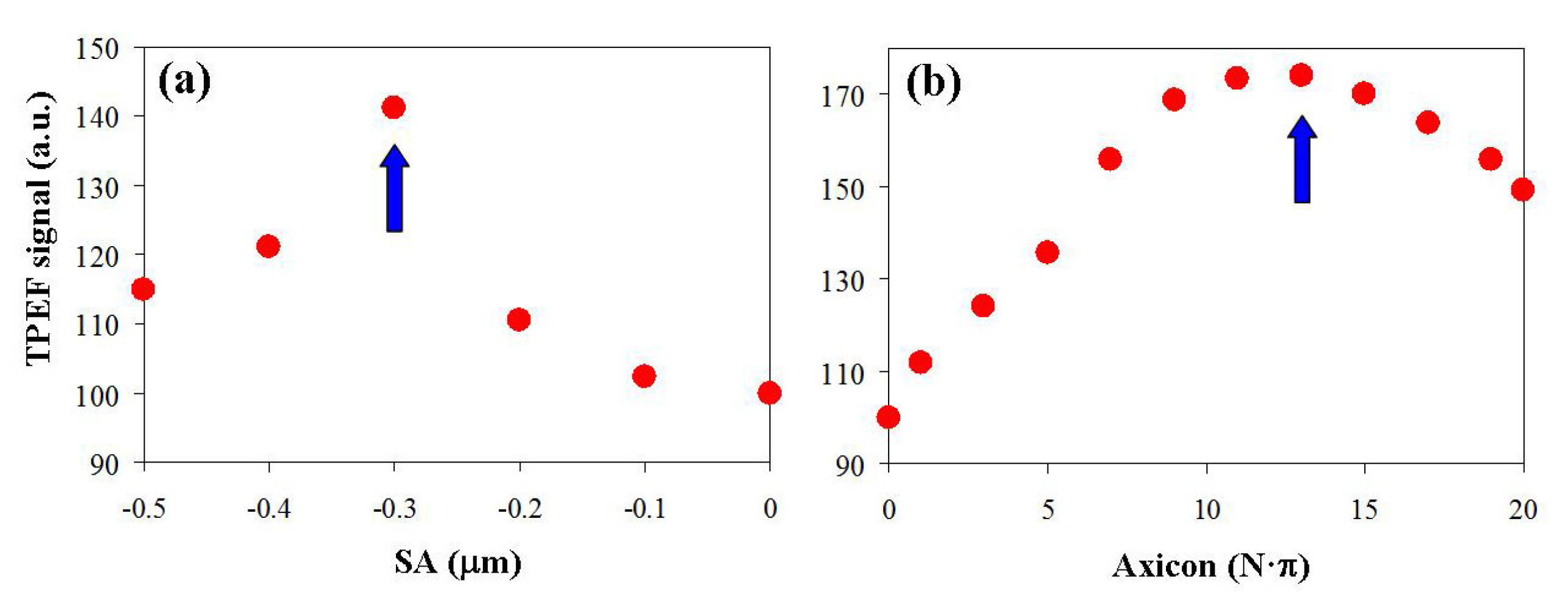
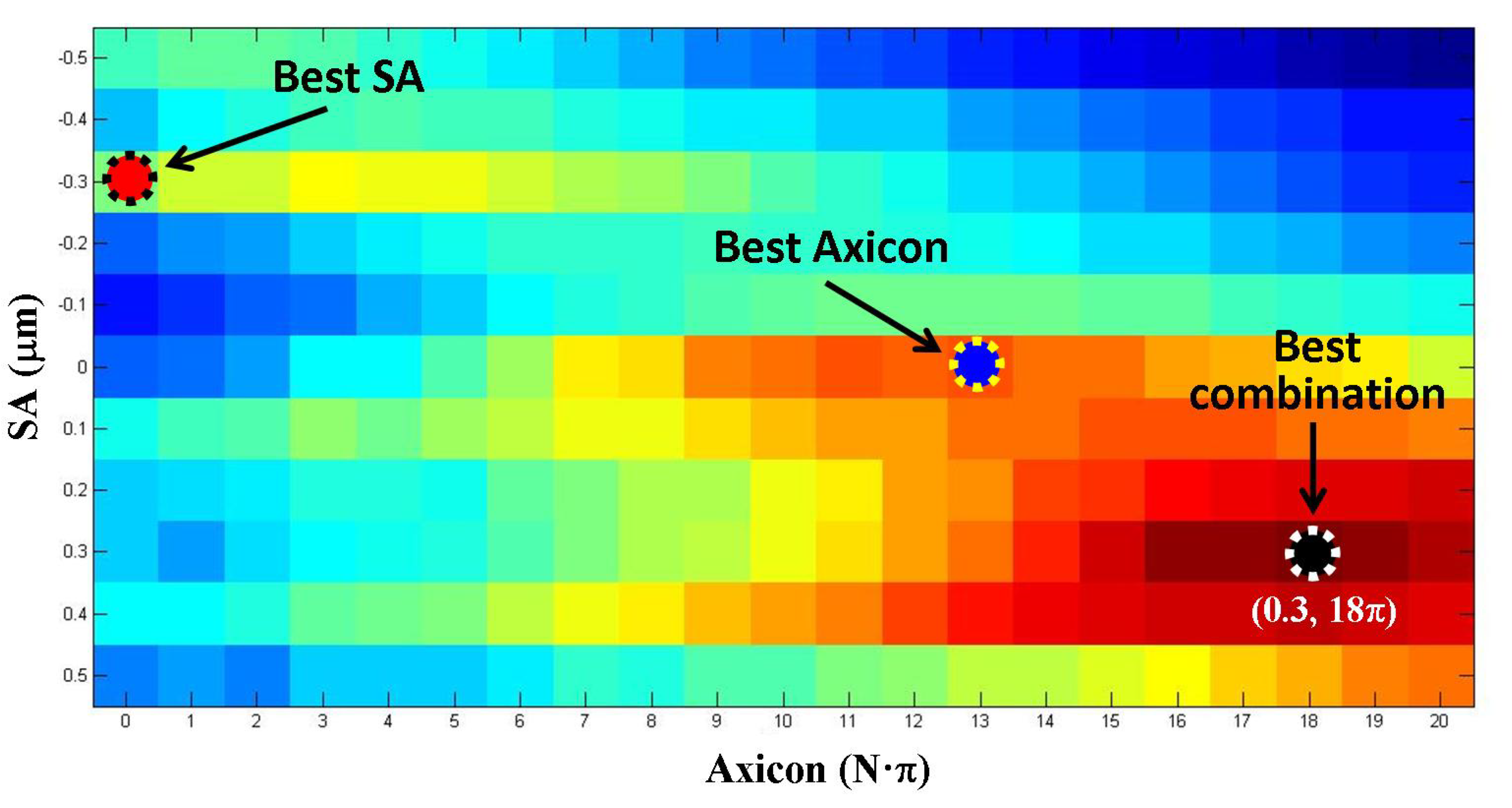
For each sample involved in the study, the experimental system was first set to sequentially record MP images at a given depth location for different amounts of SA induced by the SLM. SA values were produced in steps of 0.10 μm. From each image, the total intensity was automatically computed. The image with the highest value was considered to provide the most appropriate SA value for that depth location [5,6]. Moreover, to establish the relative impact of this optimum SA pattern, different image quality parameters were also computed (acutance, entropy, signal-to-noise ratio) [28].
A similar procedure was performed using variable axicons. These were obtained through a direct mimic of a glass axicon on the SLM [23,29]. In brief, the SLM displays a phase pattern that corresponds to the Fourier transform of the desired light field distribution (i.e., a Bessel beam) in the microscope’s objective focal plane. Positive lenses L3-L6 conjugate the SLM plane with the entrance pupil of this objective. As the size of the SLM active area is constant (5-mm in diameter), changes in the phase map (named as N·π or, alternatively, amount of axicon) are associated with changes in the cone angle of the equivalent axicon lens. Once these optimum SA and axicon values were determined, the procedure was repeated for a number of combinations of both patterns and different depth locations.

3. Results

Aberrations have a detrimental influence on the effectiveness of MP signals. This is more pronounced when the imaged plane corresponds to a deeper location within the sample. As a representative example, Figure 2 presents TPEF images within a piece of stained cellulose acquired at different depth locations. The decrease in the image quality as a function of depth can easily be observed.
This decrease in the image quality as a function of depth can be minimized by compensating for the SA value corresponding to each particular depth location. The effect of the SA on TPEF images from the same piece of cellulose is presented in Figure 3a. The imaged plane within the sample was randomly chosen (100 μm for this case). Different amounts of SA were introduced by the SLM during image acquisition. There is a particular SA value providing an image with a maximum signal. For these images, there was an improvement in the signal of 41%. As expected, this optimum value was unique for each sample and depth location.
Then, the procedure was carried out using variable axicons as explained above. The results when the SLM generates axicon phase patterns are depicted in Figure 3b. It can be observed that there also exists a value of axicon providing an optimized image. The improvement in the signal was 74%, that is, almost twice the value corresponding to the optimum SA value.
Since both the SA and axicons have been shown to enhance MP imaging, the next question would be: is it possible to combine both to further improve the effectiveness of an MP process? To answer this question, pairs of SA–axicon values were projected onto the SLM and the corresponding images acquired. The results for the same sample as in previous figures are shown in Figure 4. This is a map depicting the benefit of combining the SA and axicon patterns for a particular depth location (100 μm). The optimum values for the SA and axicon (individually) are those of Figure 3. It can be seen that, for this sample, the image provided by the best axicon presents a higher signal (see hotter color in Figure 4) than that corresponding to the optimum SA value. Moreover, the combination of both patterns leads to an image with a much better signal (97% increase).
The corresponding images are presented in Figure 5. To facilitate a direct comparison, all images share the same color scale. In addition and for the sense of completeness, Figure 6 compares the intensity profiles along the vertical line depicted in Figure 5a. The benefit when using the combination of SA and axicon is readily observable. For this particular profile, the combination SA–axicon shows an increase in both the contrast and resolution (small features not present in the original image appear in the final improved image). In addition, the parts of the image with an absence of the TPEF signal remain, which indicates that the use of different phase patterns does not introduce noise.
The two-dimensional point spread functions (2D-PSFs) corresponding to the three experimental conditions reported in Figure 5 were numerically computed. The cross sections of these 2D-PSFs are represented in Figure 7 for direct comparisons. As expected from the image improvement in the above TPEF images, the combination SA–axicon results in the narrowest PSF when compared to that of SA or axicon individually. This narrowing in the PSF leads to an increase in MP efficiency [4,5,6].
The procedure was also applied to other specimens (see Figure 8), such as a rabbit cornea embedded in paraffin (20-μm thick) and a fixed human epiretinal membrane (60-μm thick), providing SHG and TPEF signals, respectively. As shown in Figure 8, for all the samples, the use of an axicon gave better results than the use of an SA pattern. However, the combination SA–axicon led to an image that is even better than those obtained with individual patterns of either SA or axicon. The combinations of SA–axicon to optimize the images were (+0.3, 18π), (+0.1, 5π), and (+0.1, 10π) for the piece of cellulose (red bars), the rabbit cornea (blue bars), and the human epiretinal membrane (green bars), respectively.
This enhancement in the MP signal when combining SA and digital axicons is also associated with an improvement in the image quality, as different metrics indicate. The metrics used here were found to behave similarly, although the improvement value depended on each particular metric. For instance, acutance and entropy increased two-fold and 50%, respectively, when comparing images from Figure 5a,d. However, despite these differences, the final improved images were similar, as Figure 9 depicts.
Since the MP signal decreases with the sample’s depth (see Figure 2), the next step was to analyze the performance of the procedure when imaging planes were located at different depth locations. The amount of SA required to improve images from deeper planes increases with depth. This fact was also analyzed using variable axicons. As depicted in Figure 10, similar to the SA effect, the amount of axicon required to improve MP imaging also increases with depth.
Finally, a representative example of combining SA and axicons for different depth locations within the cellulose sample is plotted in Figure 11. Independent of the depth position of the imaged plane, the use of variable axicons (blue dots) provides better results than the use of SA patterns (red dots). Moreover, the combination SA–axicon gets better images than those corresponding to either SA or axicon individually (black dots). Figure 11 also includes the optimum pairs of SA–axicon for the different depths. It can be seen that, whereas the amount of axicon requires to be increased with depth, the value for SA remains constant. This finding was similar for all the samples involved here.

4. Discussion and Conclusions

An MP microscope incorporating an SLM in the illumination pathway and using a dry objective lens has been used to improve MP images at different depth locations. The SLM was programmed to generate controlled amounts of SA and variable axicons in order to increase the quality of images at different depth locations independently of the specimen-induced aberrations.
Different authors have showed the benefit of using SA compensation in MP microscopy through both static (collars) and dynamic (adaptive optics) approaches [5,6,7,8,9,10]. They reported that the SA required to get optimum MP images increases with depth [5,6] and depends on each sample under analysis.
Refractive (conical lens)-based axicons produce an axially elongated focus of a fixed axial length [12,13]. However, to investigate thick volumes, Bessel beams with variable foci are more appropriate. Different approaches have been reported to adjust this length with and without moving parts [14,16]. In addition, digital axicons using SLMs have also been successfully implemented into MP imaging applications [16,24,25]. These provided the adjustable axial extent of the imaged volume while preserving the lateral resolution in different samples, such as mouse kidney histological slides (15 μm thick) [24] and in larval zebrafish (over 60 μm depth) [16]. Moreover, a theoretical study has recently reported that the use of a Bessel beam illumination in MP microscopy imaging reduces the background from the sample surface, which can increase the penetration depth [30]. The present experiment shows that, similar to what occurs with SA, the amount of axicon required to acquire the best MP image also increases at deeper locations (the thickest sample used here was 100 μm thick).
Unlike those previous experiments, the technique presented here takes a step forward and combines variable axicons without mobile parts and SA correction. This merges the benefit of generating the optimum Bessel focus for each location of interest together with the compensation of the SA effects, which contributes to further improving the focal spot, then increases the MP efficiency and provides better images.
The most interesting result reported here is that an accurate manipulation of the combination of SA and axicon provides noticeable MP imaging improvement. This enhancement is higher than that reached when using SA or variable axicons separately. Although the optimum combination depended on both the sample and the depth location, for the samples involved here, the increase in the signal ranged between 38% and five-fold. Moreover, it is worthwhile to notice that the best image hardly depended on the image quality metric used (see Figure 9).
The improvement in the MP signal (as measured with different metrics) was more noticeable at deep regions. Then, this effect might be understood as an increase in the imaging depth or extended depth of focus and has been demonstrated in samples providing both TPEF and SHG signals. Consequently, this appropriate combination of both patterns leads to a more efficient imaging and would permit the use of lower illumination levels, reducing the risk of damage in biological samples.
Because the samples used here are static, the time required to complete the procedure is not an issue. This agrees with other wavefront sensor-less algorithms, such genetic or simulated annealing [31]. Since the actual experimental system is not optimized for speed, the main drawback of the proposed technique is the number of iterations used. Although, in the present form, this would limit its use with dynamic samples, future implementations (including reduced and optimized recording times) will speed the procedure up, as previously reported by others [5,7,16,25,32,33]. This may lead to new applications with great possibilities for in vivo MP imaging.
In conclusion, this work reports what we believe is the first experimental combination of SA and variable axicon patterns into an MP microscope. This procedure has been shown to enhance image quality independently on the depth location of the imaged plane. Since the phase patterns are projected on an SLM (i.e., a physical axicon is not required), this offers a flexible, reliable, and accurate imaging procedure. This approach offers a new perspective on volumetric imaging and might optimize the MP performance at deeper layers in a number of research fields, ranging from the ocular imaging of thick tissues to the visualization of complex neuronal networks.

Author Contributions

Conceptualization and experiment design, J.M.B. and P.A.; experimental measurements, J.M.B., G.H., and M.S.; data curation and analysis, G.H. and M.S.; draft preparation, J.M.B.; writing and review, J.M.B. and P.A. All authors have read and agreed to the published version of the manuscript.

Funding

This work was supported by the Agencia Estatal de Investigación, Spain (grants PID2019-105684RB-I00 and PID2020-113919RB-I00).

Institutional Review Board Statement

Not applicable.

Informed Consent Statement

Not applicable.

Data Availability Statement

Requests for materials should be addressed to J.M.B.

Acknowledgments

The authors thank Pedro Prieto for helpful assistance and discussions on the PSF improvement.

Conflicts of Interest

The authors declare no conflict of interest.

References

  1. Denk, W.; Strickler, J.H.; Webb, W.W. Two-photon laser scanning fluorescence microscopy. Science 1990, 248, 73–76. [Google Scholar] [CrossRef] [Green Version]
  2. Guo, Y.; Ho, P.P.; Savage, H.; Harris, D.; Sacks, P.; Schantz, S.; Liu, F.; Zhadin, N.; Alfano, R.R. Second-harmonic tomography of tissues. Opt. Lett. 1997, 22, 1323–1325. [Google Scholar] [CrossRef]
  3. Sherman, L.; Ye, J.Y.; Albert, O.; Norris, T.B. Adaptive correction of depth-induced aberrations in multiphoton scanning microscopy using a deformable mirror. J. Microsc. 2002, 206, 65–71. [Google Scholar] [CrossRef]
  4. Booth, M.J. Adaptive optical microscopy: The ongoing quest for a perfect image. Light Sci. Appl. 2014, 3, e165. [Google Scholar] [CrossRef]
  5. Débarre, D.; Botcherby, E.J.; Watanabe, T.; Srinivas, S.; Booth, M.J.; Wilson, T. Image-based adaptive optics for two-photon microscopy. Opt. Lett. 2009, 34, 2495–2497. [Google Scholar] [CrossRef] [Green Version]
  6. Skorsetz, M.; Artal, P.; Bueno, J.M. Performance evaluation of a sensor-less adaptive optics multiphoton microscope. J. Microsc. 2015, 261, 249–258. [Google Scholar] [CrossRef] [PubMed]
  7. Bueno, J.M.; Skorsetz, M.; Palacios, R.; Gualda, E.J.; Artal, P. Multiphoton imaging microscopy at deeper layers with adaptive optics control of spherical aberration. J. Biomed. Opt. 2014, 19, 011007. [Google Scholar] [CrossRef]
  8. Lo, W.; Sun, Y.; Lin, S.-J.; Jee, S.-H.; Dong, C.-Y. Spherical aberration correction in multiphoton fluorescence imaging using objective correction collar. J. Biomed. Opt. 2005, 10, 034006. [Google Scholar] [CrossRef]
  9. Muriello, P.A.; Dunn, K.W. Improving signal levels in intravital multiphoton microscopy using an objective correction collar. Opt. Commun. 2008, 281, 1806–1812. [Google Scholar] [CrossRef] [PubMed] [Green Version]
  10. Matsumoto, N.; Inoue, T.; Matsumoto, A.; Okazaki, S. Correction of depth-induced spherical aberration for deep observation using two-photon excitation fluorescence microscopy with spatial light modulator. Biomed. Opt. Express 2015, 6, 2575–2587. [Google Scholar] [CrossRef] [PubMed] [Green Version]
  11. Botcherby, E.J.; Juskaitis, R.; Wilson, T. Scanning two photon fluorescence microscopy with extended depth of field. Opt. Commun. 2006, 268, 253–260. [Google Scholar] [CrossRef]
  12. Thériault, G.; De Koninck, Y.; McCarthy, N. Extended depth of field microscopy for rapid volumetric two-photon imaging. Opt. Express 2013, 21, 10095–10104. [Google Scholar] [CrossRef]
  13. Dufour, P.; Piché, M.; De Koninck, Y.; McCarthy, N. Two-photon excitation fluorescence microscopy with a high depth of field using an axicon. Appl. Opt. 2006, 45, 9246–9252. [Google Scholar] [CrossRef] [PubMed]
  14. Thériault, G.; Cottet, M.; Castonguay, A.; McCarthy, N.; De Koninck, Y. Extended two-photon microscopy in live samples with Bessel beams: Steadier focus, faster volume scans, and simpler stereoscopic imaging. Front. Cell. Neurosci. 2014, 8, 139. [Google Scholar]
  15. Dumin, J.; Miceli, J.J., Jr.; Eberly, J.H. Diffraction-free beams. Phys. Rev. Lett. 1987, 58, 1499–1501. [Google Scholar]
  16. Lu, R.; Tanimoto, M.; Koyama, M.; Ji, N. 50 Hz volumetric functional imaging with continuously adjustable depth of focus. Biomed. Opt. Express 2018, 9, 1964–1976. [Google Scholar] [CrossRef] [Green Version]
  17. Vasara, A.; Turunen, J.; Friberg, A.T. Realization of general nondiffracting beams with computer-generated holograms. J. Opt. Soc. Am. A 1989, 6, 1748–1754. [Google Scholar] [CrossRef]
  18. Davis, J.A.; Carcole, E.; Cottrell, D.M. Nondiffracting interference patterns generated with programmable spatial light modulators. Appl. Opt. 1996, 35, 599–602. [Google Scholar] [CrossRef] [Green Version]
  19. Bowman, R.; Muller, N.; Zambrana-Puyalto, X.; Jedrkiewicz, O.; Di Trapani, P.; Padgett, M.J. Efficient generation of Bessel beam arrays by means of an SLM. Eur. Phys. J. Spec. Top. 2011, 199, 159–166. [Google Scholar] [CrossRef] [Green Version]
  20. Trichili, A.; Mhlanga, T.; Ismail, Y.; Roux, F.; McLaren, M.; Zghal, M.; Forbes, A. Detection of Bessel beams with digital axicons. Opt. Express 2014, 22, 17553–17560. [Google Scholar] [CrossRef] [Green Version]
  21. Chattrapiban, N.; Rogers, E.; Cofield, D.; Hill, W., III; Roy, R. Generation of nondiffracting Bessel beams by use of a spatial light modulator. Opt. Lett. 2003, 28, 2183–2185. [Google Scholar] [CrossRef] [PubMed]
  22. García-Martínez, P.; Sánchez-López, M.M.; Davis, J.A.; Cottrell, D.M.; Sand, D.; Moreno, I. Generation of Bessel beam arrays through Dammann gratings. Appl. Opt. 2012, 51, 1375–1381. [Google Scholar] [CrossRef]
  23. Ventura, M.E.M.; Tapang, G.A.; Saloma, C.A. Robust Bessel beam scanning without mechanical movement. Proc. SPIE 2016, 9896, 989618. [Google Scholar]
  24. Vuillemin, N.; Mahou, P.; Débarre, D.; Gacoin, T.; Tharaux, P.-L.; Schanne-Klein, M.-C.; Supatto, W.; Beaurepaire, E. Efficient second-harmonic imaging of collagen in histological slides using Bessel beam excitation. Sci. Rep. 2016, 6, 29863. [Google Scholar] [CrossRef] [PubMed]
  25. Lu, R.; Sun, W.; Liang, Y.; Kerlin, A.; Bierfeld, J.; Seelig, J.D.; Wilson, D.E.; Scholl, B.; Nohar, B.; Tanomoto, M.; et al. Video-rate volumetric functional imaging of the brain at synaptic resolution. Nat. Neurosci. 2017, 20, 620–628. [Google Scholar] [CrossRef] [PubMed] [Green Version]
  26. Lu, R.; Liang, Y.; Meng, G.; Zhou, P.; Svoboda, K.; Paninski, L.; Ji, N. Rapid mesoscale volumetric imaging of neural activity with synaptic resolution. Nat. Methods 2020, 17, 291–294. [Google Scholar] [CrossRef]
  27. Bueno, J.M.; Skorsetz, M.; Bonora, S.; Artal, P. Wavefront correction in two-photon microscopy with a multiactuator adaptive lens. Biomed. Opt. Express 2018, 26, 14278–14287. [Google Scholar] [CrossRef]
  28. Hunter, J.J.; Cookson, C.J.; Kisilak, M.L.; Bueno, J.M.; Campbell, M.C.W. Characterizing image quality in a scanning laser ophthalmoscope with differing pinholes and induced scattered light. J. Opt. Soc. Am. A 2007, 24, 1284–1295. [Google Scholar] [CrossRef] [Green Version]
  29. Fahrbach, F.O.; Gurchenkov, V.; Alessandri, K.; Nassoy, P.; Rohrbach, A. Light-sheet microscopy in thick media using scanned Bessel beams and two-photon fluorescence excitation. Opt. Express 2013, 21, 13824–13839. [Google Scholar] [CrossRef] [Green Version]
  30. Sheppard, C.J.R.; Castello, M.; Tortarolo, G.; Slenders, E.; Deguchi, T.; Koho, S.V.; Vicidomini, G.; Diaspro, A. Image scanning microscopy with multiphoton excitation or Bessel beam illumination. J. Opt. Soc. Am. A 2020, 37, 1639–1649. [Google Scholar] [CrossRef]
  31. Wright, A.J.; Burns, D.; Patterson, B.A.; Poland, S.P.; Valentine, G.J.; Girkin, J.M. Exploration of the optimisation algorithms used in the implementation of adaptive optics in confocal and multiphoton microscopy. Microsc. Res. Tech. 2005, 67, 36–44. [Google Scholar] [CrossRef]
  32. Olivier, N.; Débarre, D.; Beaurepaire, E. Dynamic aberration correction for multiharmonic microscopy. Opt. Lett. 2009, 34, 3145–3147. [Google Scholar] [CrossRef]
  33. Ávila, F.J.; Gambín, A.; Artal, P.; Bueno, J.M. In vivo two-photon microscopy of the human eye. Sci. Rep. 2019, 9, 10121. [Google Scholar] [CrossRef] [Green Version]
Figure 1. Schematic diagram of the MP microscope used for the purpose of this work. L1–L6, lenses; M1–M3, mirrors; DM, dichroic mirror; SLM, spatial light modulator; PMT, photo-multiplier tube. Further details about the different components and optical elements can be found in [6,27].
Photonics 08 00573 g001
Figure 2. TPEF images recorded at different depth locations (0 (a), 40 (b), and 100 (c) μm). Samples correspond to a piece of cellulose stained with DAPI (4′,6-diamidino-2-phenylindole). Bar length: 50 μm. The reduction in TPEF signal between (a) and (c) was 83%.
Photonics 08 00573 g002
Figure 3. TPEF intensity values as a function of the amount of SA (a) and variable axicon (b) introduced by the SLM. The arrows indicate the optimum experimental conditions. The imaged plane is located at 100 μm within the sample.
Photonics 08 00573 g003
Figure 4. Map of TPEF signal for different combinations of SA and axicon. The sample is the same piece of cellulose used in previous figures.
Photonics 08 00573 g004
Figure 5. TPEF images of the cellulose sample (100 μm depth) recorded before (a) and after using the optimum values of SA (b), axicon (c), and pair SA–axicon (d). Bar length: 50 μm.
Photonics 08 00573 g005
Figure 6. Intensity profiles along the vertical line indicated in Figure 5a showing the benefit of an optimized combination of SA and variable axicon (black line). Green line: original; red line: only SA.
Photonics 08 00573 g006
Figure 7. Cross sections through the PSFs for optimum combinations of SA (red), axicon (blue), and SA+axicon (black) in Figure 5.
Photonics 08 00573 g007
Figure 8. Improvement in MP signal for the samples used herein. Red, blue, and green bars correspond to a piece of cellulose (that of Figure 5), a rabbit cornea (upper panels), and an epiretinal membrane (bottom panels), respectively. Original images are shown on the (left). (Right) panels are the improved images for the optimum combinations of SA–axicon.
Photonics 08 00573 g008
Figure 9. TPEF (top panels, piece of cellulose) and SHG (bottom panels, rabbit cornea) images corresponding to the best combinations of SA+axicon when optimizing acutance (a,c) and entropy (b,d). Bar length: 50 μm. These images are very similar to those obtained when optimizing the signal, and depicted in Figure 5d and Figure 8 (top right panel).
Photonics 08 00573 g009
Figure 10. Improvement in TPEF signal as a function of depth using variable axicons. The results correspond to a piece of cellulose.
Photonics 08 00573 g010
Figure 11. Comparison of MP signal improvement as a function of depth when using SA (red), axicon (blue), or an optimum combination of both (white).
Photonics 08 00573 g011
Publisher’s Note: MDPI stays neutral with regard to jurisdictional claims in published maps and institutional affiliations.

