Numerical Study of Resonant Optical Parametric Amplification via Gain Factor Optimization in Dispersive Microresonators

Abstract
:1. Introduction
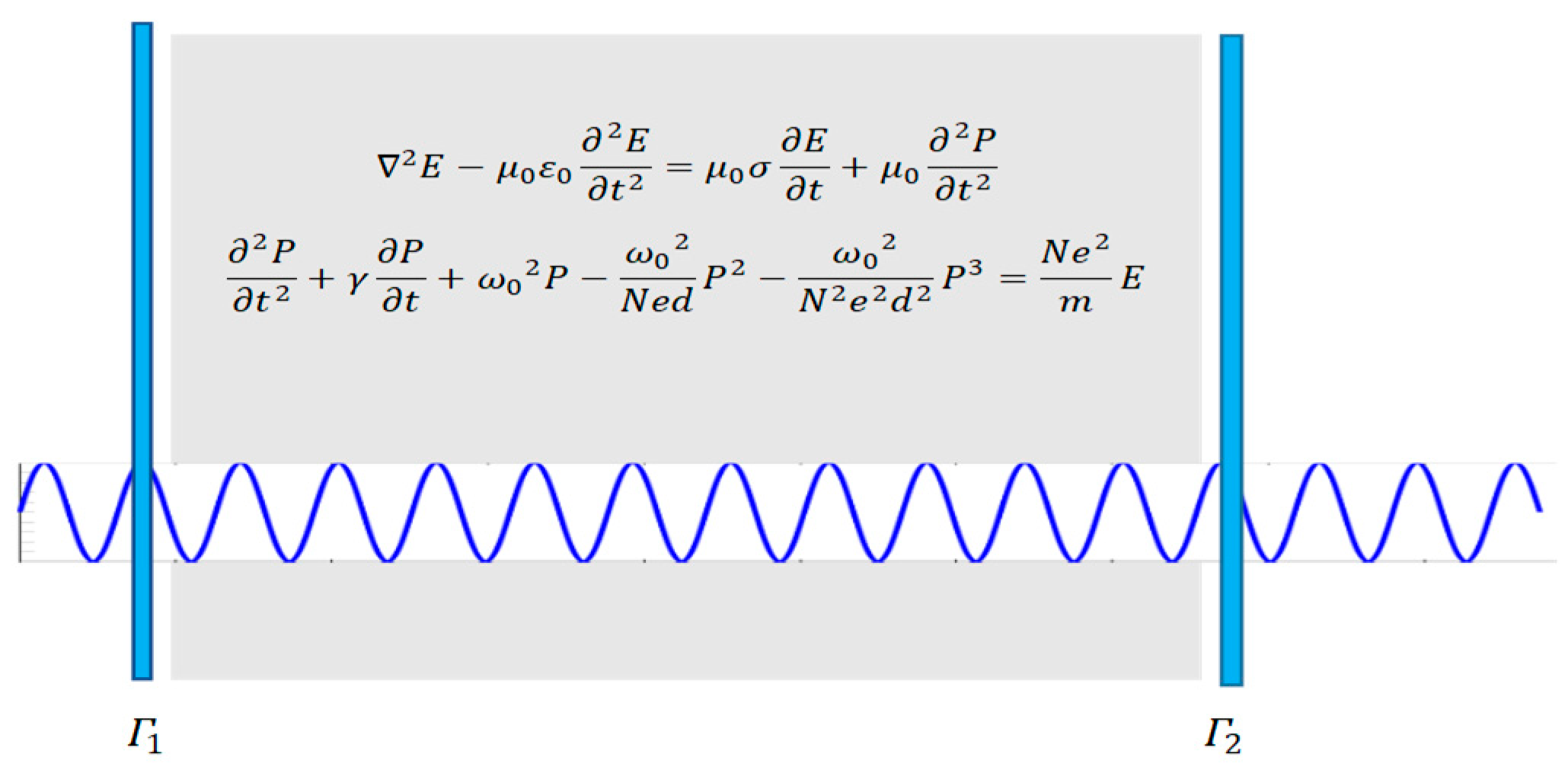
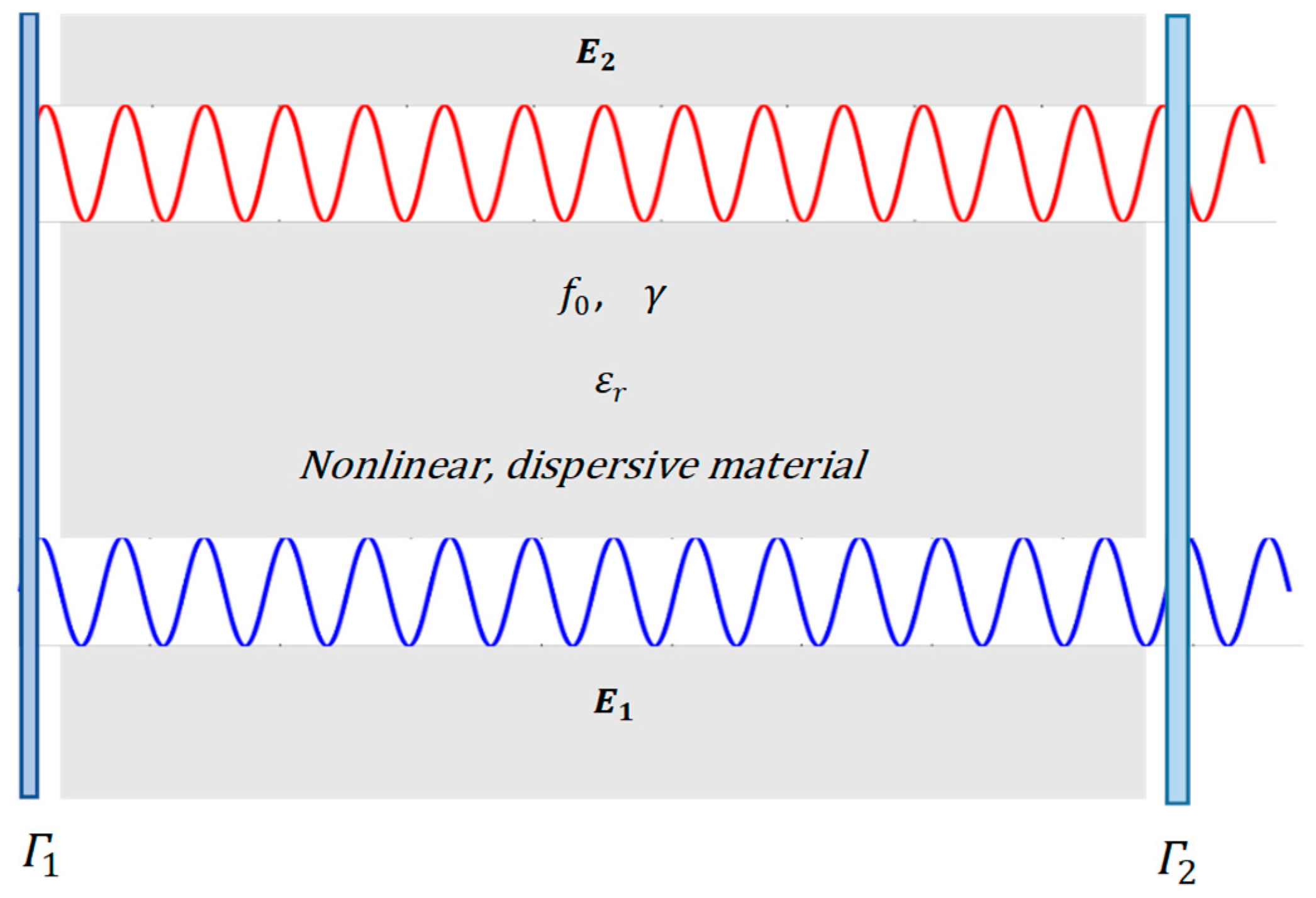
2. Wave Propagation in Nonlinear Dispersive Media
3. Optimization of Optical Parametric Amplification Gain Performance
4. Finite Difference Time Domain Formulation Based Solution of the Gain Factor Optimization Problem in Optical Parametric Amplification
5. Simulation Results
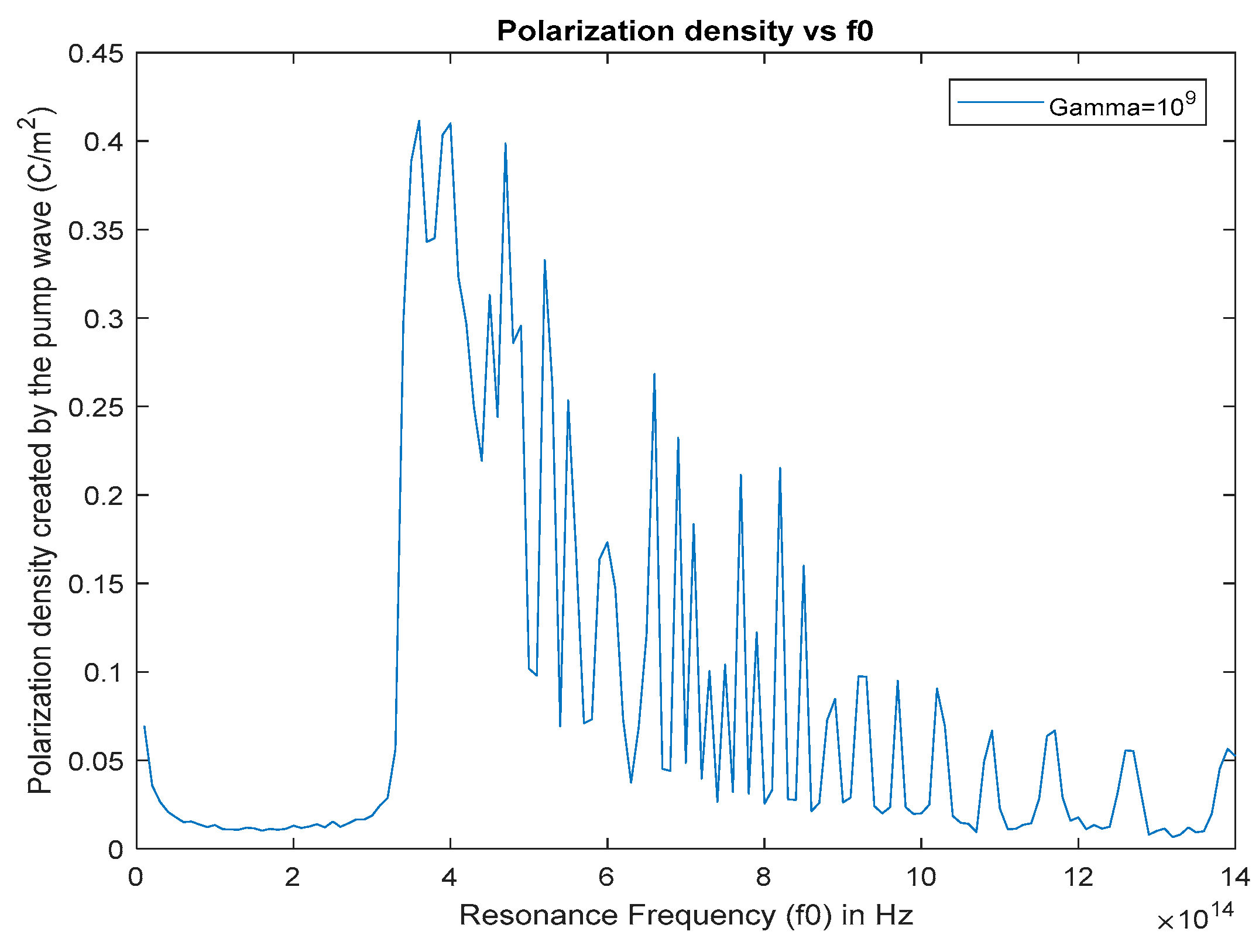
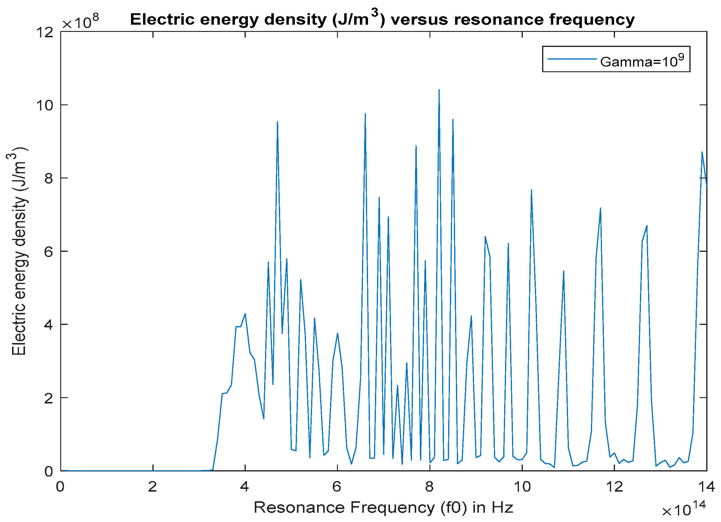
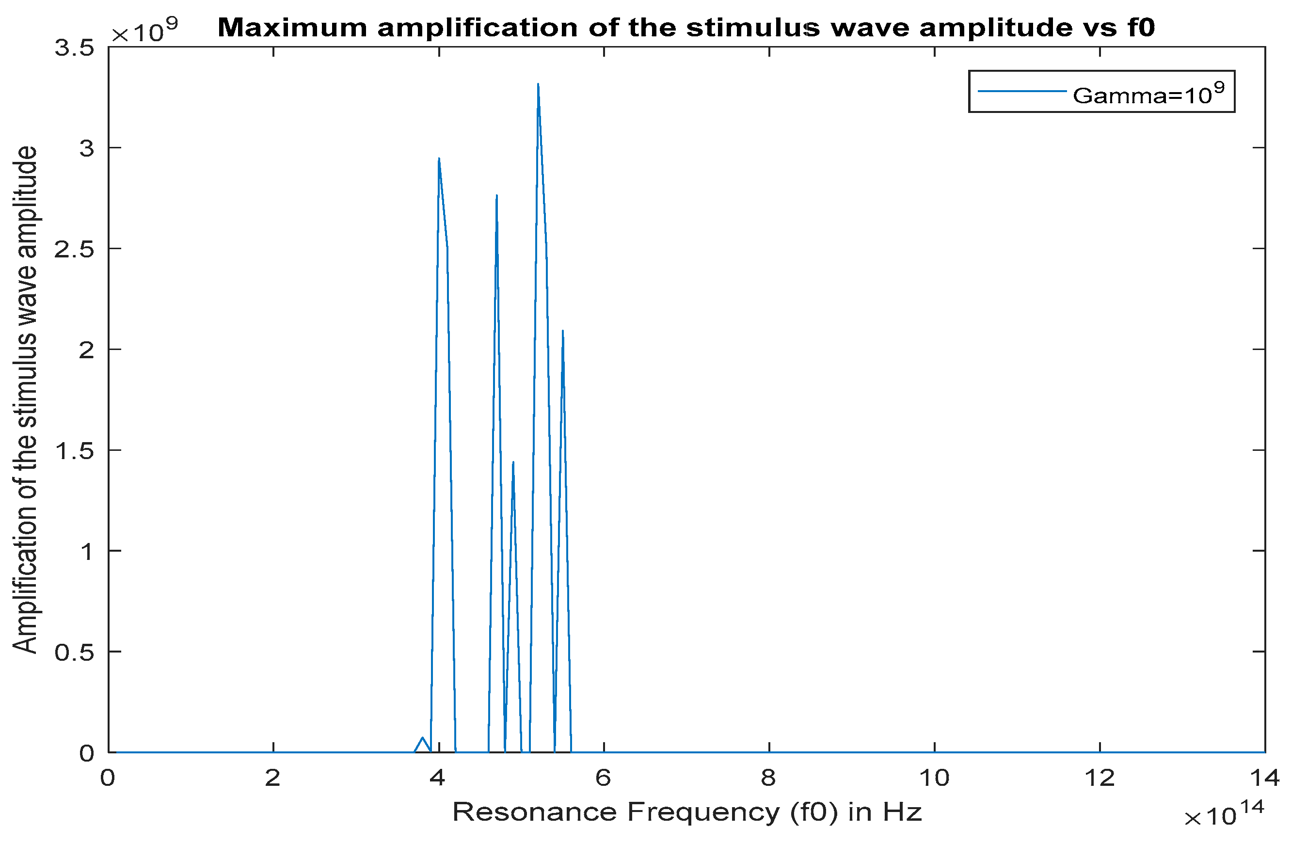
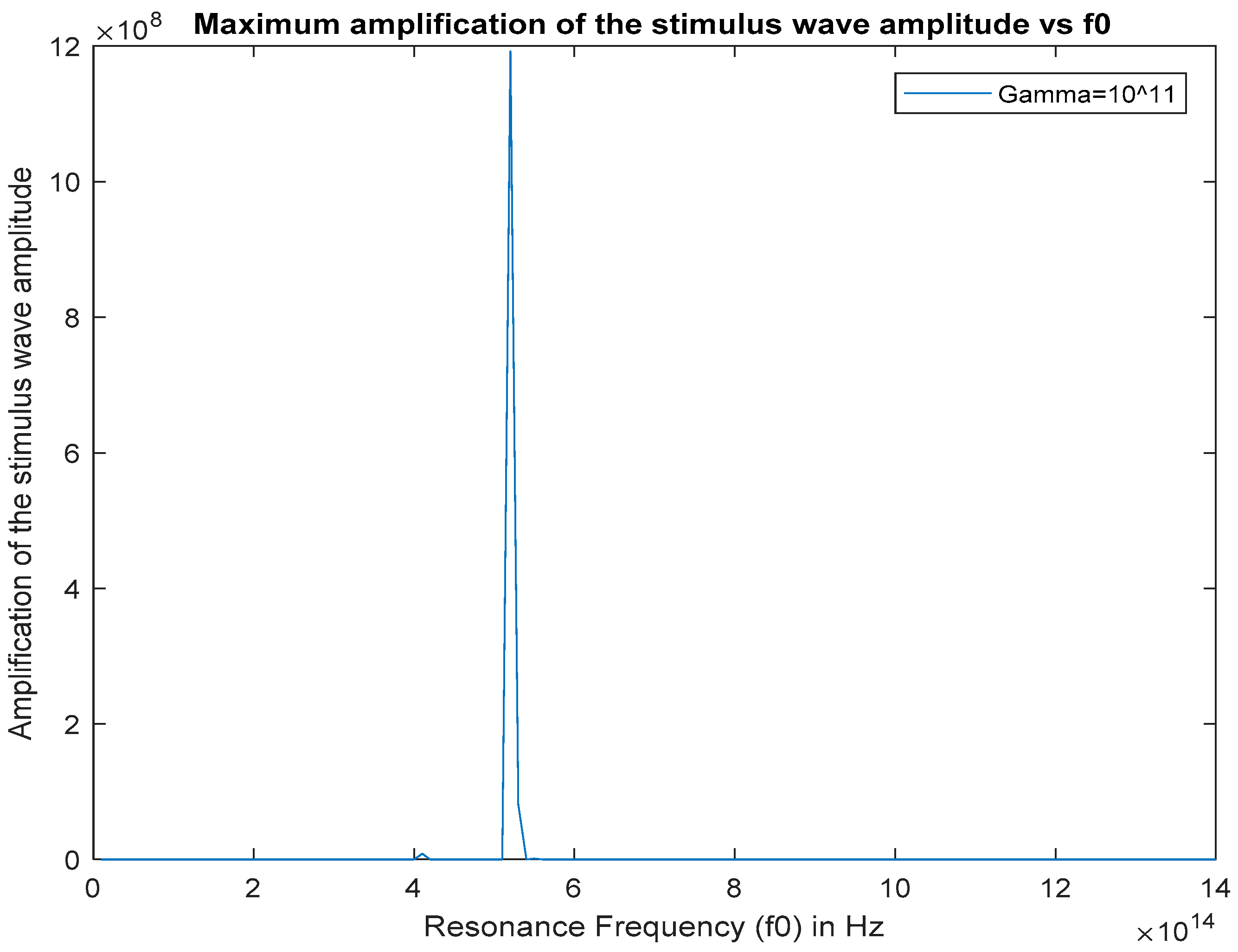
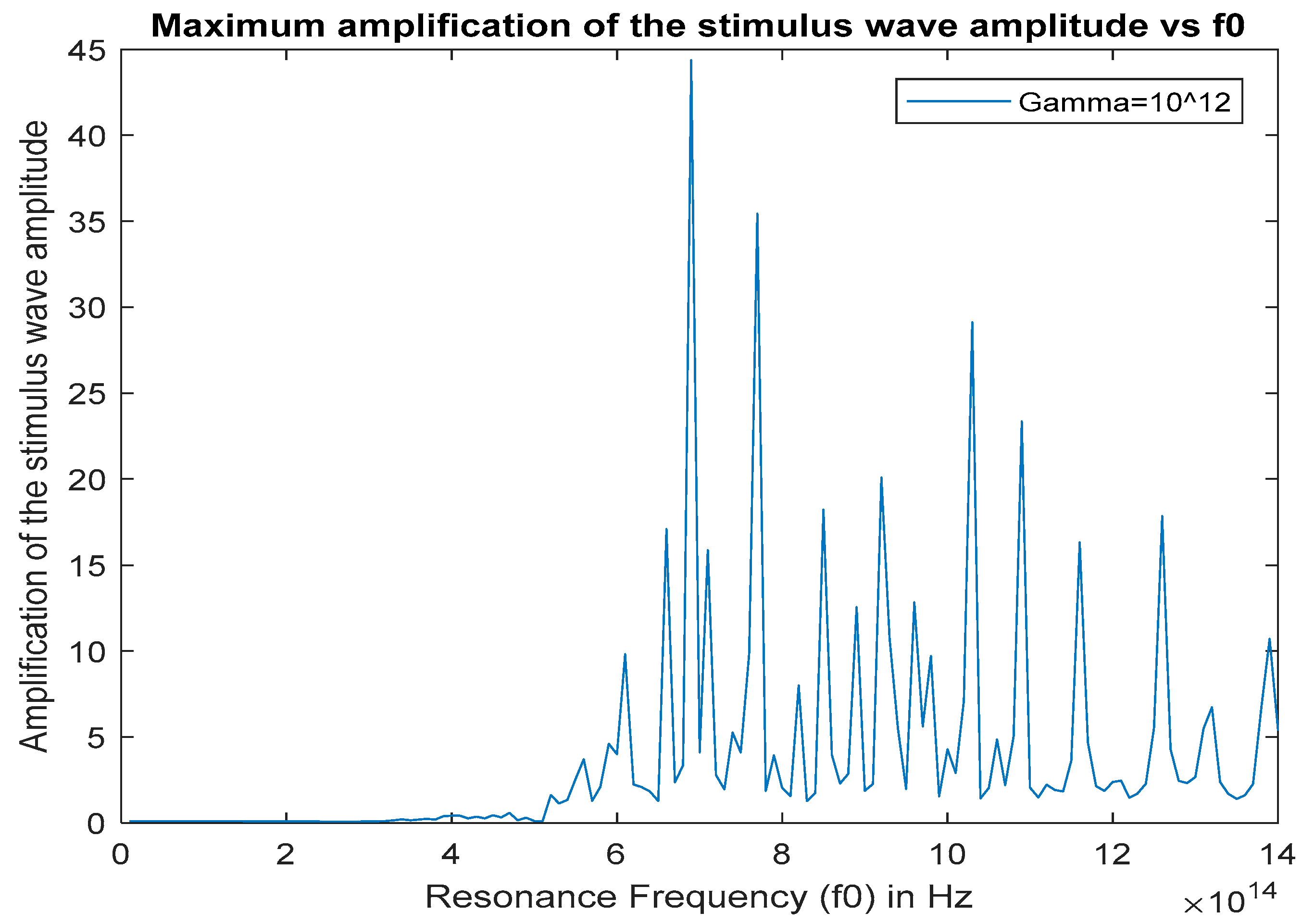
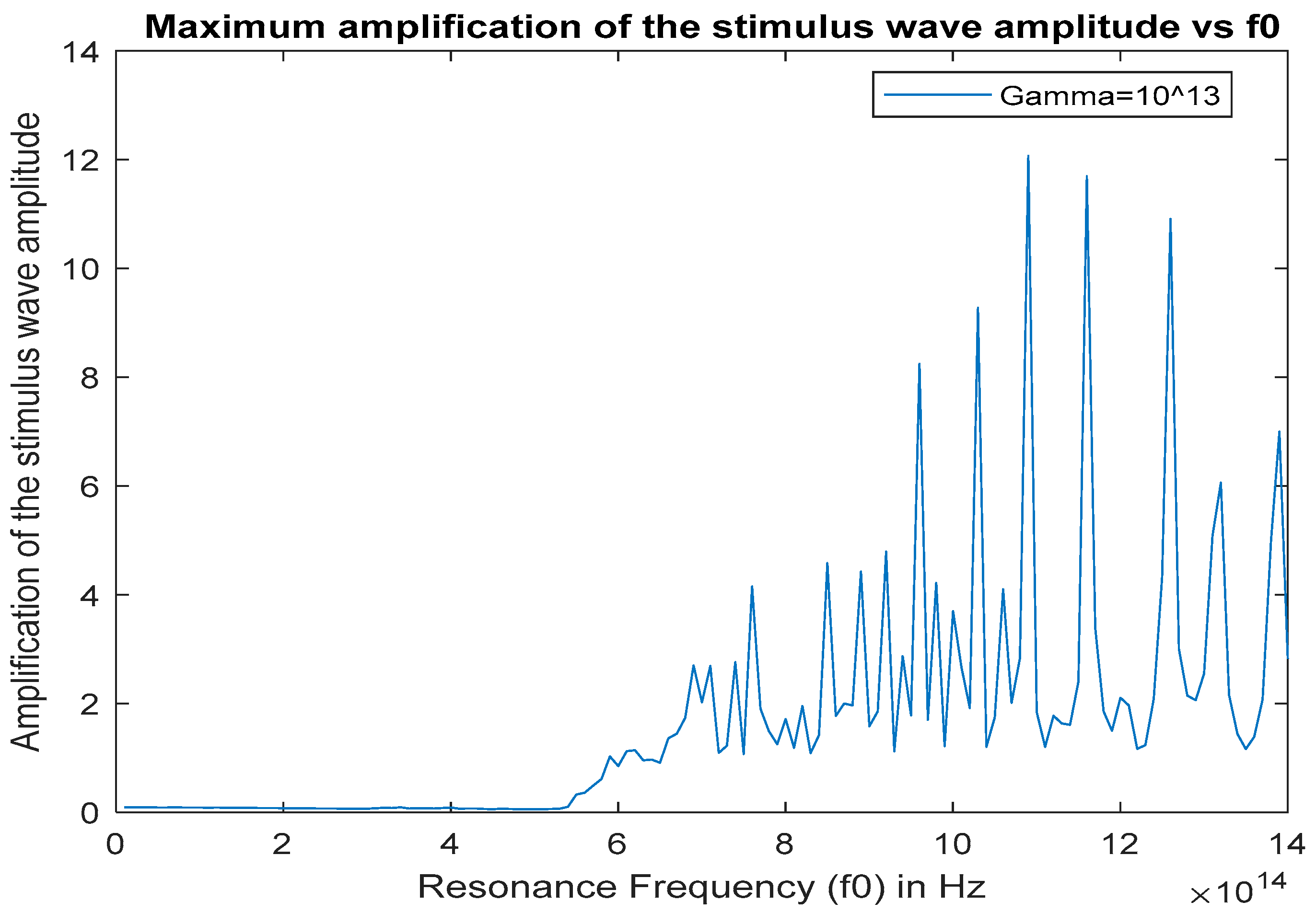
5.1. Finding the Optimal Resonance Frequency for High Gain Optical Parametric Amplification
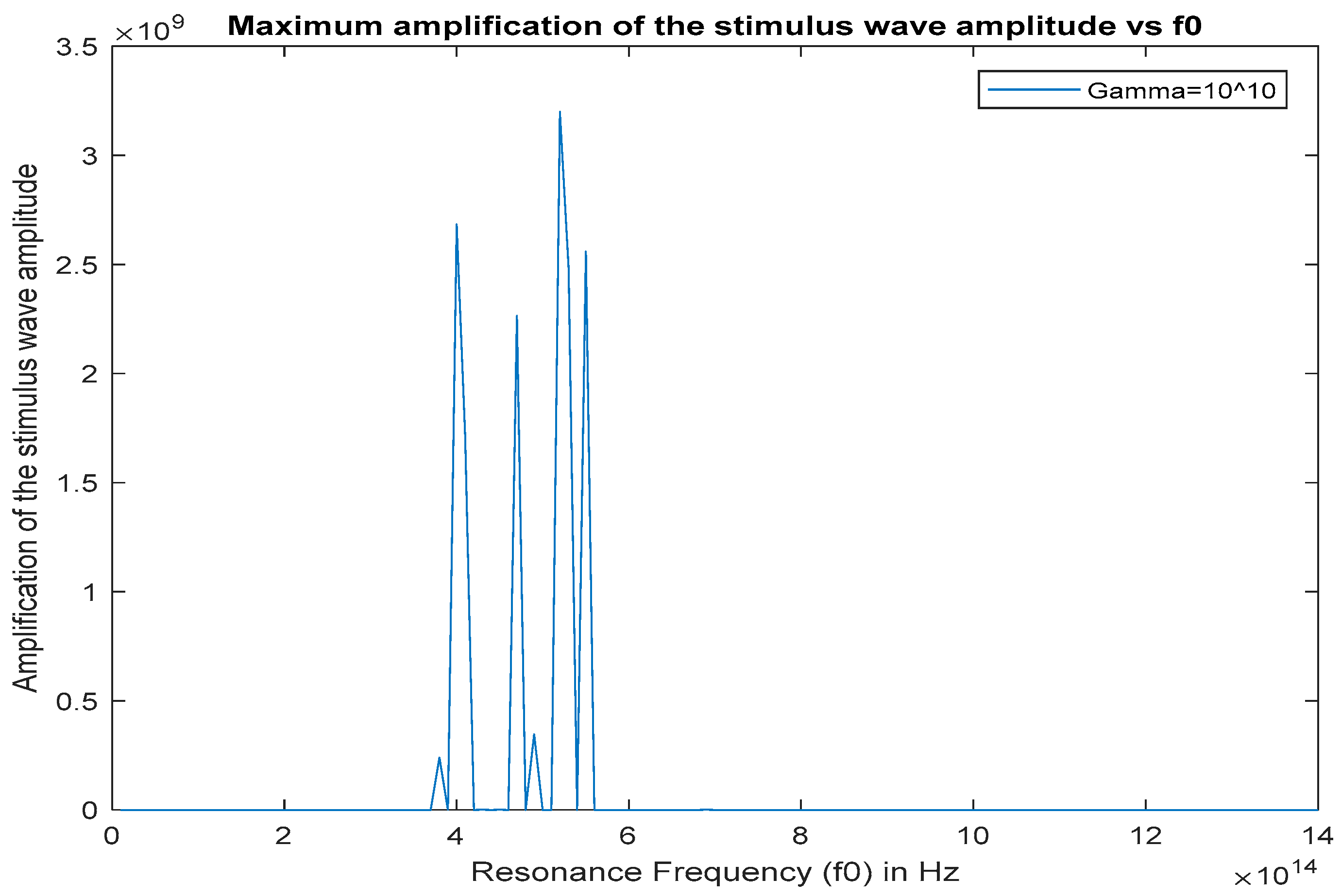
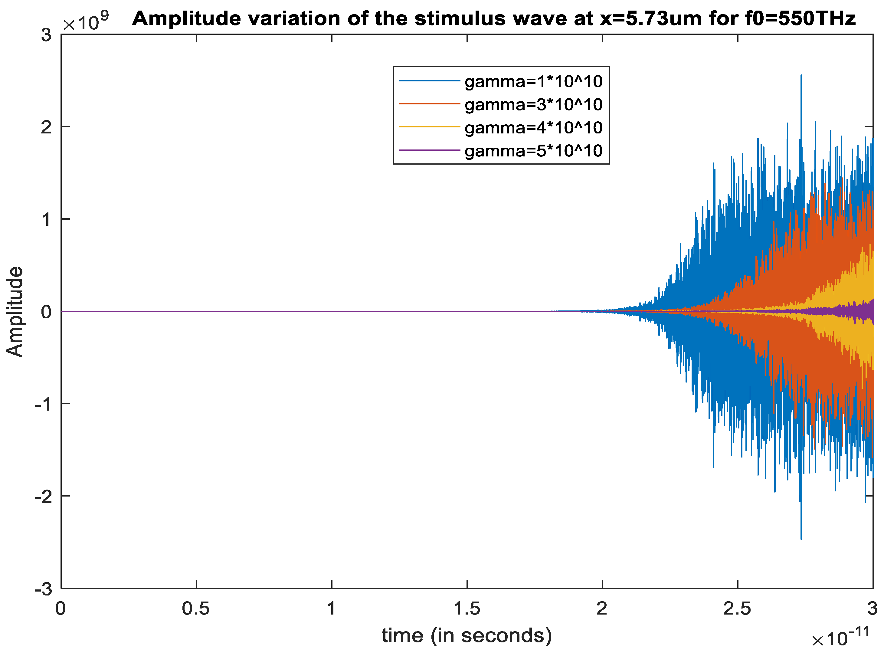
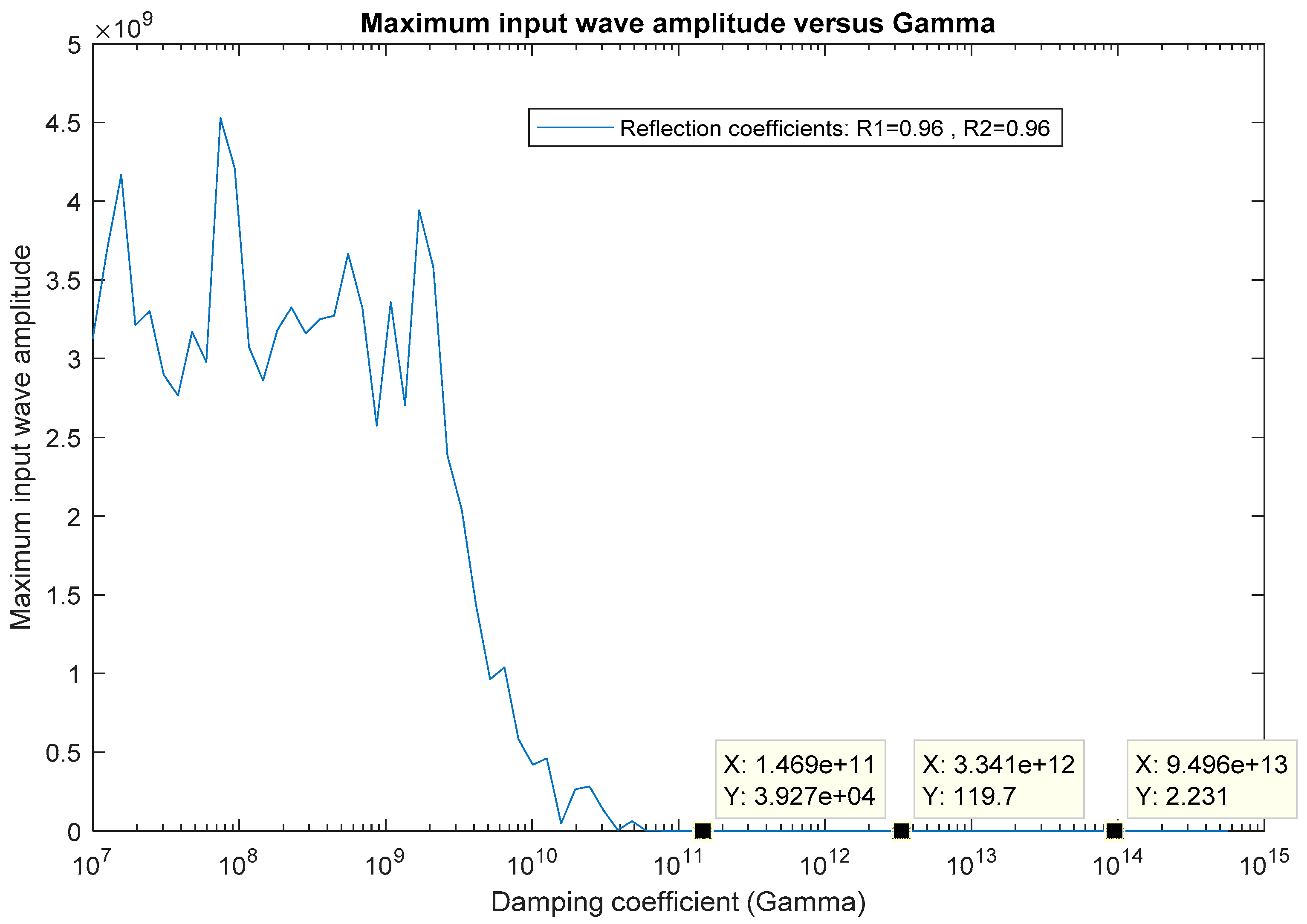
5.2. Effect of the Damping Coefficient on Stimulus Wave Amplification
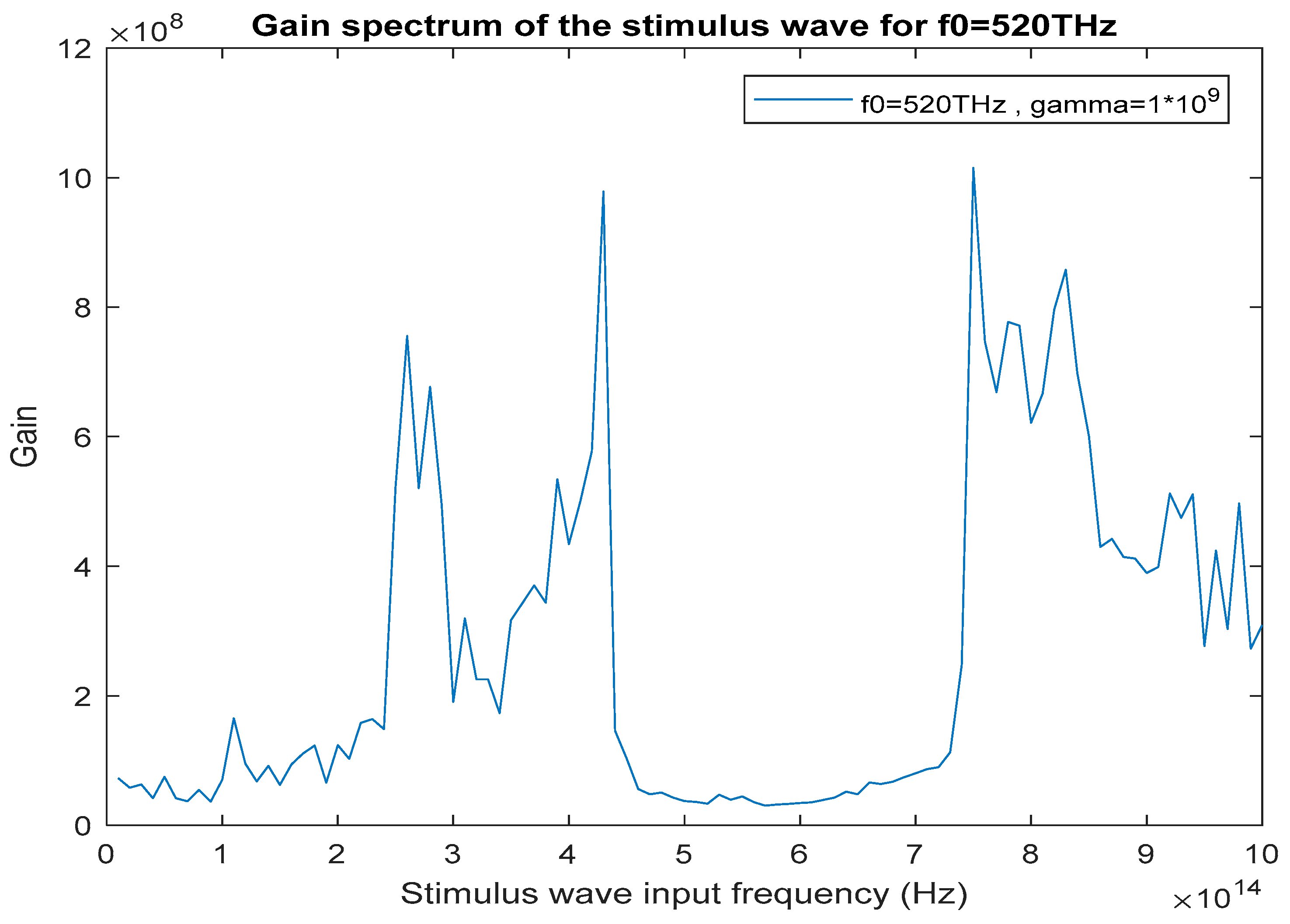
5.3. Analyzing the Gain Spectrum of the Stimulus Wave at the Optimal Resonance Frequency
- (1)
- Based on our computations, changing the length of the cavity, or the length of the gain medium, does not change the spectral gain resonance locations.
- (2)
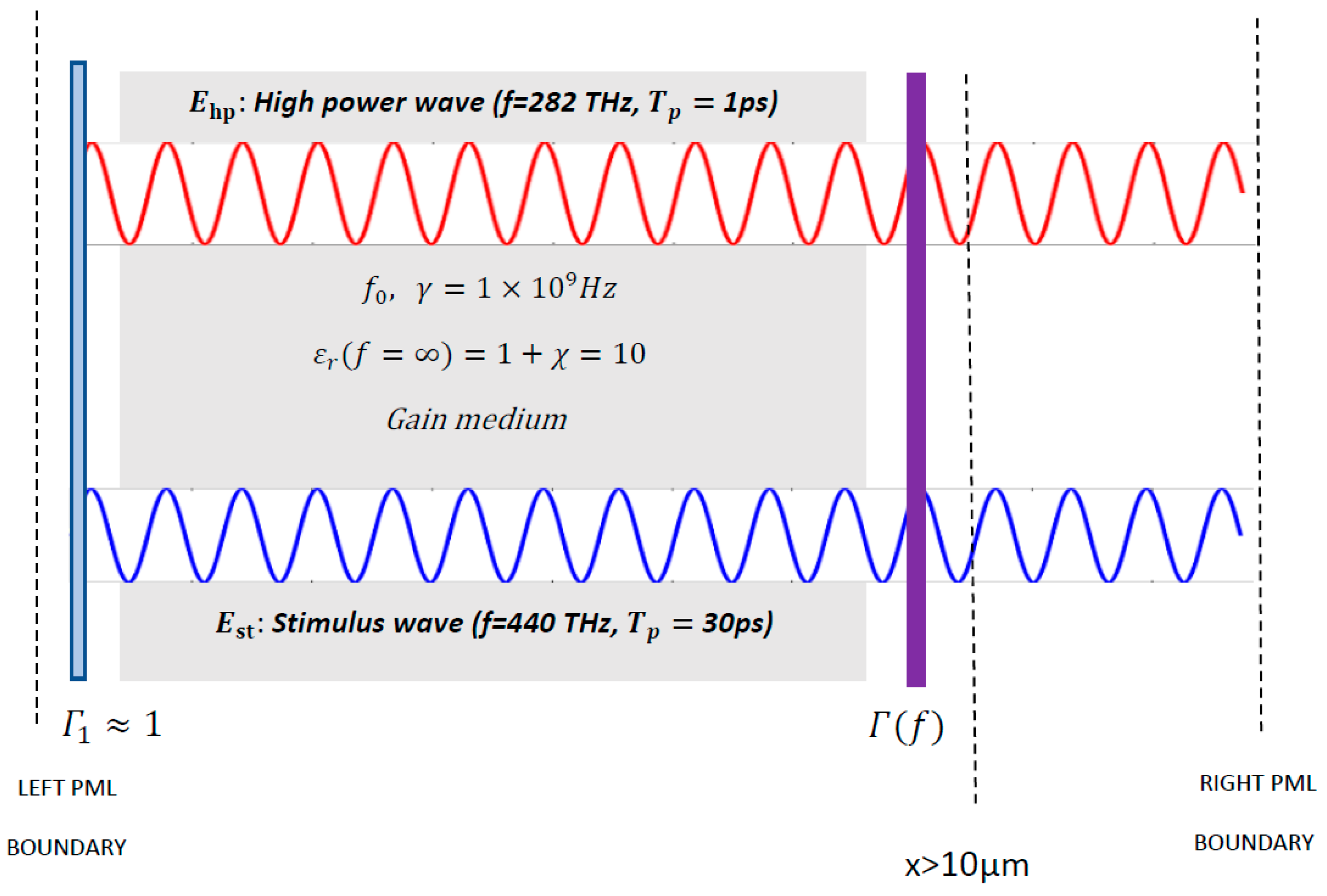
- The amplitude ( of the pump wave is the typical electric field amplitude of a focused 1.064 wavelength ultrashort Nd:YAG laser beam, which corresponds to an optical intensity of . Dielectric breakdown in dispersive media occurs at an optical intensity level of and beyond. Therefore, at this amplitude the pump wave would not induce dielectric breakdown and would not pose an optical hazard to the medium of interaction [13,14,15].
- (3)
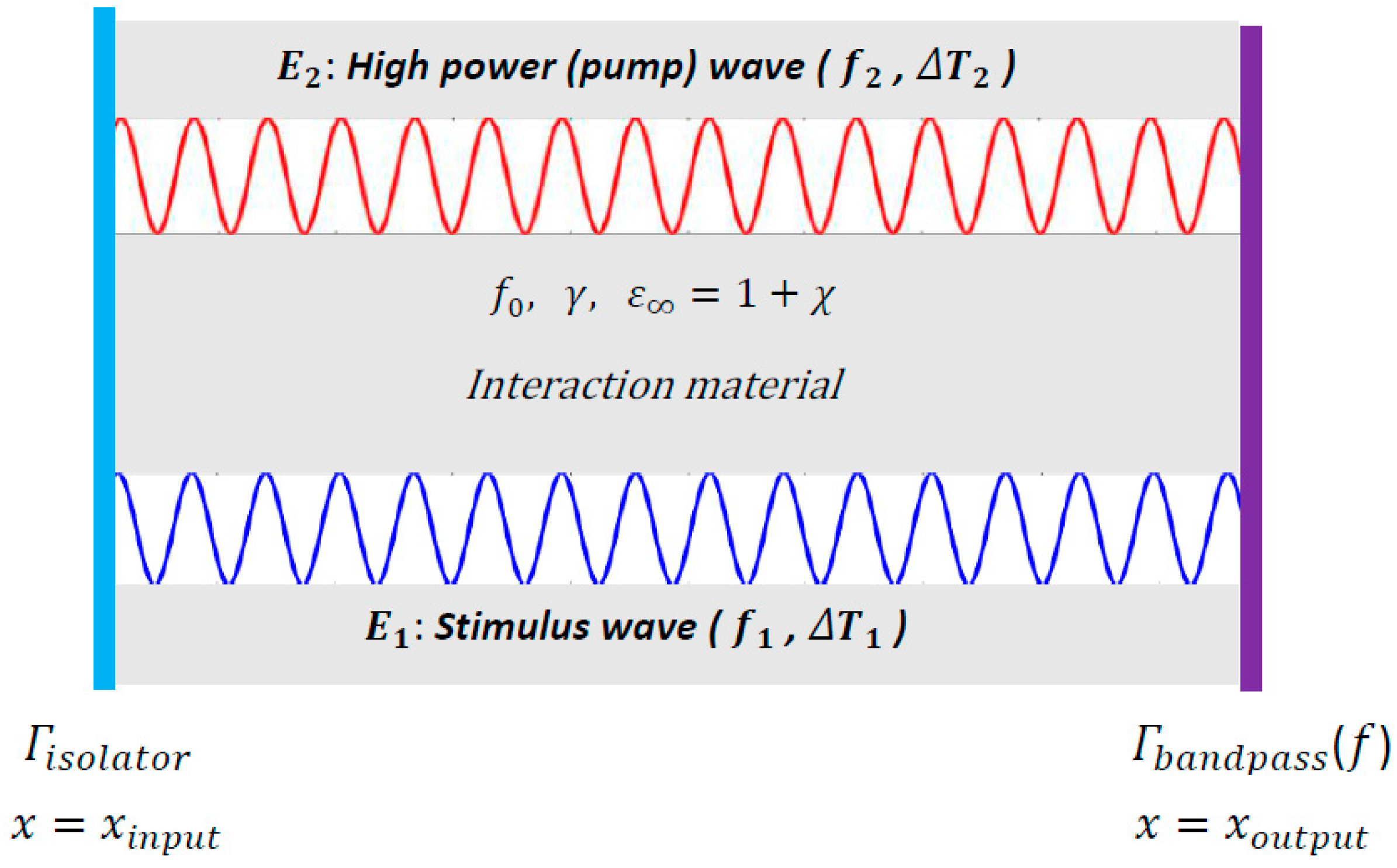
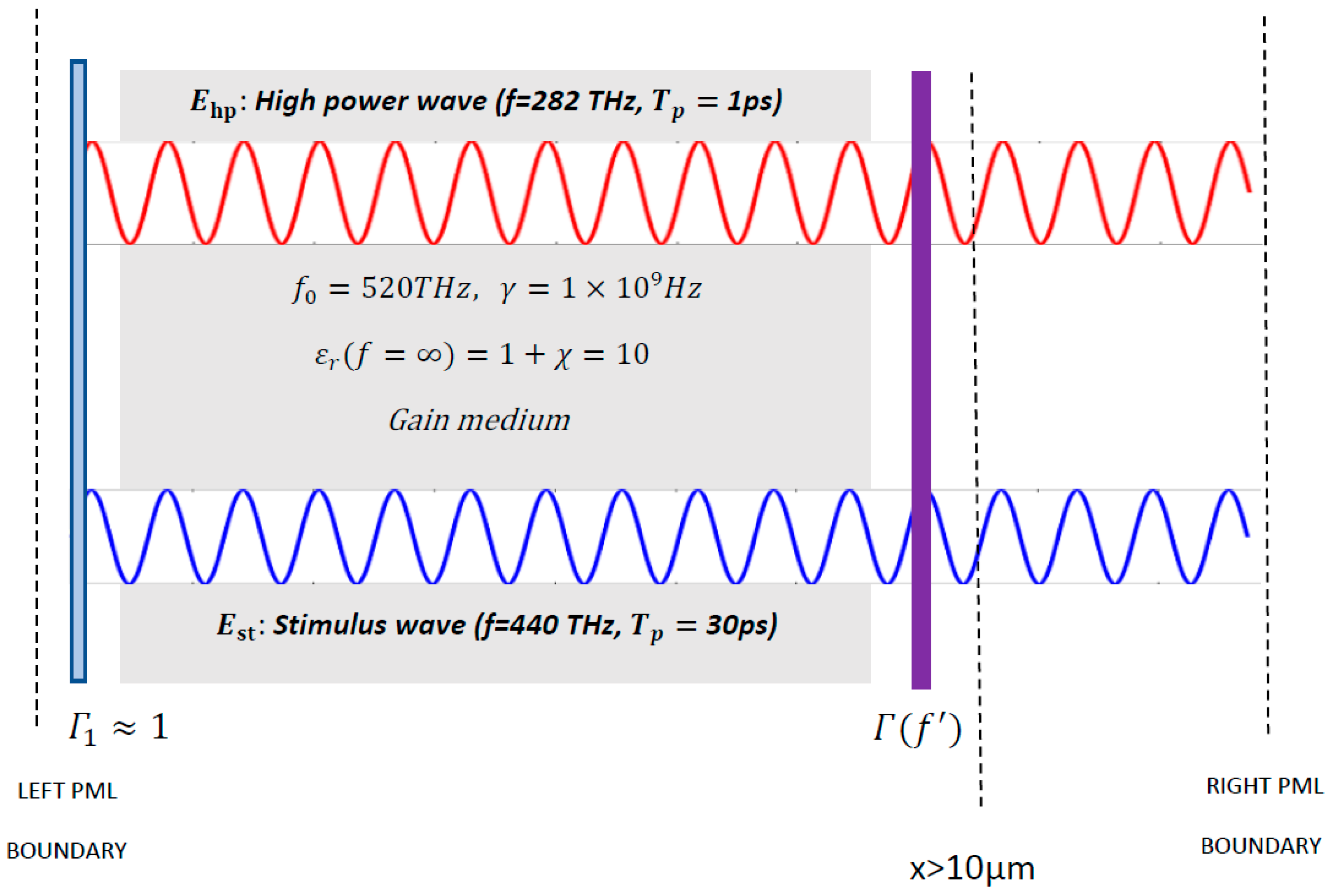
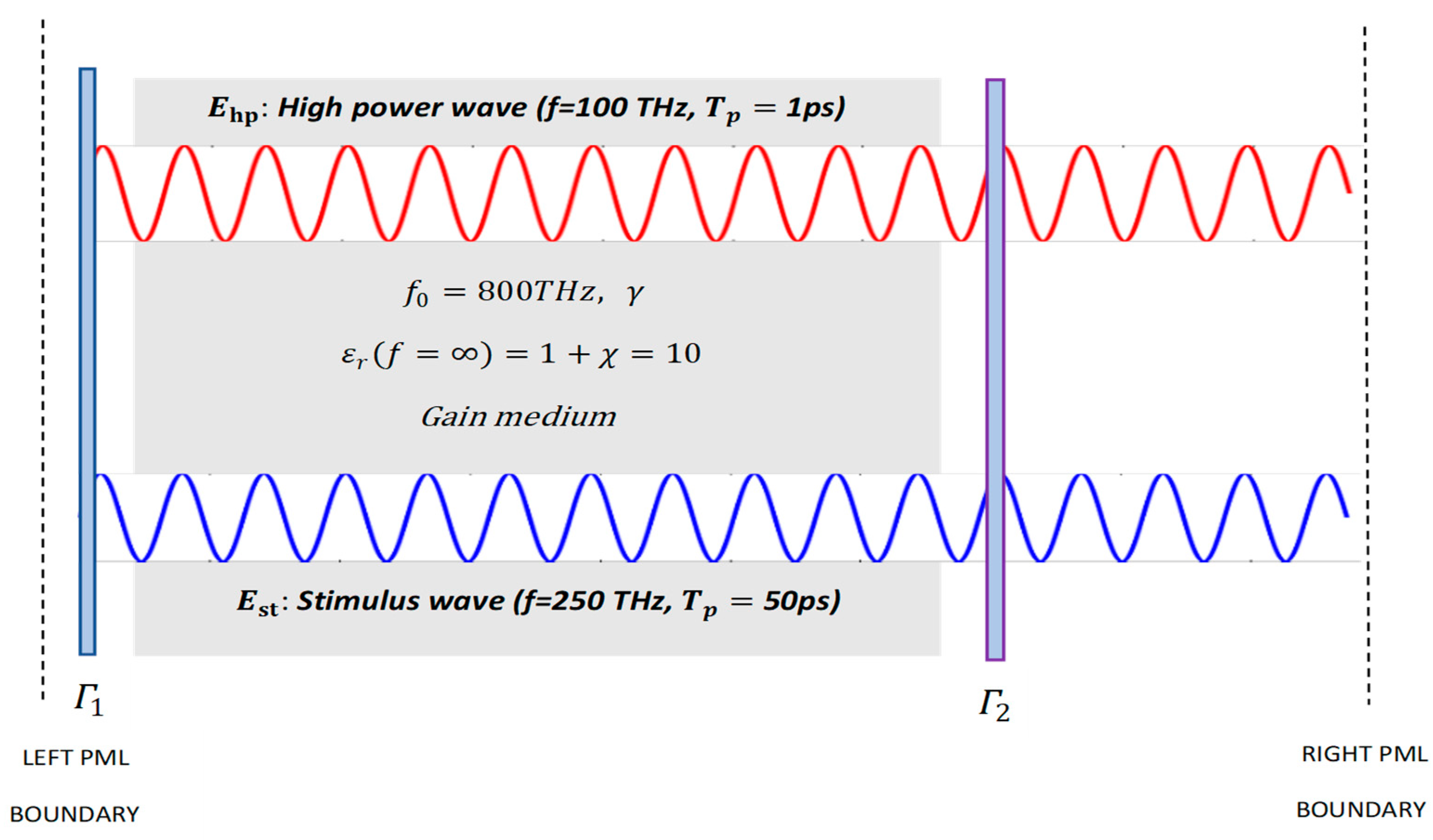
- The temporal walk-off between the interacting waves that stems from the dispersion of the medium limits the effective interaction length. To counter-act this effect, we should ensure that the reflection losses at the cavity walls are minimized. The optical isolator that is used as a cavity wall should be of high quality to maximize intracavity reflections (. The bandpass transmission filter reflection coefficient must be maximized at the optical transmission stopband, so that the stored electric energy is retained in the cavity to support the high-gain amplification of the stimulus wave. In this paper we have assumed that the optical isolator (left cavity wall) reflection coefficient is 1 from the inside of the cavity (ideal optical isolator), and the reflection coefficient of the filter (right cavity wall) is close to 1 at the transmission stopband. When the reflection losses are minimized, the number of round trips in the cavity for which the nonlinearity is retained, is maximized and the reduced effective interaction length due to temporal walk-off between the interacting waves is compensated.
5.4. Effect of the Damping Coefficient and the Mean Cavity Wall Reflection Coefficient on Optical Parametric Amplification
6. Conclusions
- The cavity should be low loss. This is satisfied in our computations by choosing a dielectric gain medium , and by adjusting the reflectivities of the cavity walls to be very high.
- The damping coefficient (polarization decay rate) of the gain medium should be low ().
- The resonance frequency of the gain medium must match with one of the resonance frequencies that are found to maximize the stimulus wave gain inside the cavity. In the case of a 282 THz Nd:YAG pump wave excitation, the resonance frequency of the interaction material should reside between 350 THz and 600 THz (350 THz < .
- Bithiophene based red fluorescent light emitting material called BTCN, which has a resonance frequency value of 470 THz with a FWHM bandwidth of 80 THz, is a suitable interaction medium for resonant optical parametric amplification using a 282 THz Nd:YAG pump wave excitation.
Author Contributions
Funding
Conflicts of Interest
Appendix A. Verification of Our Computational Model


References
- Boyd Robert, W. Nonlinear Optics; Academic Press: New York, NY, USA, 2008; pp. 105–107. [Google Scholar]
- Mark, F. Optical Properties of Solids; Oxford University Press: New York, NY, USA, 2002; pp. 237–239. [Google Scholar]
- Balanis Constantine, A. Advanced Engineering Electromagnetics; John Wiley & Sons: New York, NY, USA, 1989; pp. 66–67. [Google Scholar]
- Saleh, B.E.; Teich, M.C. Fundamentals of Photonics; Wiley-Interscience: New York, NY, USA, 2007; pp. 885–917. [Google Scholar]
- Silfvast William, T. Laser Fundamentals; Cambridge University Press: New York, NY, USA, 2004; pp. 24–35. [Google Scholar]
- Satsuma, J.; Yajima, N. Initial Value Problems of One-Dimensional Self-Modulation of Nonlinear Waves in Dispersive Media. Prog. Theor. Phys. Suppl. 1974, 55, 284–306. [Google Scholar] [CrossRef]
- Xu, K. Integrated Silicon Directly Modulated Light Source Using p-Well in Standard CMOS Technology. IEEE Sens. J. 2016, 16, 6184–6191. [Google Scholar] [CrossRef]
- Taflove, A.; Hagness, S.C. Computational Electrodynamics: The Finite-Difference Time-Domain Method; Artech House: Boston, MA, USA, 2005; pp. 353–361. [Google Scholar]
- Xu, K. Silicon MOS Optoelectronic Micro-Nano Structure Based on Reverse-Biased PN Junction. Phys. Status Solidi A Appl. Mater. Sci. 2019, 216, 1800868. [Google Scholar] [CrossRef] [Green Version]
- Maksymov, I.S.; Sukhorukov, A.A.; Lavrinenko, A.V.; Kivshar, Y.S. Comparative Study of FDTD-Adopted Numerical Algorithms for Kerr Nonlinearities. IEEE Antennas Wirel. Propag. Lett. 2011, 10, 143–146. [Google Scholar] [CrossRef]
- Ozgun, O.; Kuzuoglu, M. Near-field performance analysis of locally-conformal perfectly matched absorbers via Monte Carlo simulations. J. Comput. Phys. 2007, 227, 1225–1245. [Google Scholar] [CrossRef]
- Mohan, M.; Satyanarayan, M.N.; Trivedi, D.R. Bithiophene based red light emitting material -Photophysical and DFT studies. In AIP Conference Proceedings; AIP Publishing: Melville, NY, USA, 2019; Volume 2115, p. 030577. [Google Scholar]
- Ciriolo, A.G.; Negro, M.; Devetta, M.; Cinquanta, E.; Faccialà, D.; Pusala, A.; Vozzi, C. Optical Parametric Amplification Techniques for the Generation of High-Energy Few-Optical-Cycles IR Pulses for Strong Field Applications. Appl. Sci. 2017, 7, 265. [Google Scholar] [CrossRef] [Green Version]
- Migal, E.A.; Potemkin, F.V.; Gordienko, V.M. Highly efficient optical parametric amplifier tunable from near-to mid-IR for driving extreme nonlinear optics in solids. Opt. Lett. 2017, 42, 5218–5221. [Google Scholar] [CrossRef] [PubMed]
- Wu, C.; Fan, J.; Chen, G.; Jia, S. Symmetry-breaking-induced dynamics in a nonlinear microresonator. Opt. Express 2019, 27, 28133–28142. [Google Scholar] [CrossRef] [PubMed]
- Lee, S.B.; Bark, H.S.; Jeon, T. Enhancement of THz resonance using a multilayer slab waveguide for a guided-mode resonance filter. Opt. Express 2019, 27, 29357–29366. [Google Scholar] [CrossRef] [PubMed]
- el Dirani, H.; Youssef, L.; Petit-Etienne, C.; Kerdiles, S.; Grosse, P.; Monat, C.; Pargon, E.; Sciancalepore, C. Ultralow-loss tightly confining Si3N4 waveguides and high-Q microresonators. Opt. Express 2019, 27, 30726–30740. [Google Scholar] [CrossRef] [PubMed]
- Izadi, M.A.; Nouroozi, R. Adjustable Propagation Length Enhancement of the Surface Plasmon Polariton Wave via Phase Sensitive Optical Parametric Amplification. Sci. Rep. 2018, 8, 15495. [Google Scholar] [CrossRef] [PubMed]
- Chen, J.Y.; Ma, Z.H.; Sua, Y.M.; Li, Z.; Tang, C.; Huang, Y.P. Ultra-efficient frequency conversion in quasi-phase-matched lithium niobate microrings. Optica 2019, 6, 1244–1245. [Google Scholar] [CrossRef]
- Sua, Y.M.; Chen, J.Y.; Huang, Y.P. Ultra-wideband and high-gain parametric amplification in telecom wavelengths with an optimally mode-matched PPLN waveguide. Opt. Lett. 2018, 43, 2965–2968. [Google Scholar] [CrossRef] [PubMed]
- Luo, R.; He, Y.; Liang, H.; Li, M.; Ling, J.; Lin, Q. Optical Parametric Generation in a Lithium Niobate Microring with Modal Phase Matching. Phys. Rev. Appl. 2019, 11, 034026. [Google Scholar] [CrossRef] [Green Version]


| k (Iteration #) | |||||
|---|---|---|---|---|---|
| 100 THz | 8 | 2.37 | 282 THz | 1 | |
| 145 THz | 8 | 5.26 | 282 THz | 4 | |
| 173 THz | 8 | 8.78 | 282 THz | 7 | |
| 286 THz | 8 | 9.60 | 282 THz | 10 | |
| 222 THz | 8 | 10.48 | 282 THz | 13 | |
| 257 THz | 8 | 2.76 | 282 THz | 16 | |
| 341 THz | 8 | 81.53 | 282 THz | 19 | |
| 308 THz | 8 | 42.80 | 282 THz | 22 | |
| 395 THz | 8 | 1.74 | 282 THz | 25 | |
| 364 THz | 8 | 2.28 | 282 THz | 28 | |
| 422 THz | 8 | 1.95 | 282 THz | 31 | |
| 478 THz | 8 | 9.11 | 282 THz | 34 | |
| 446 THz | 8 | 4.47 | 282 THz | 37 | |
| 543 THz | 8 | 3.58 | 282 THz | 40 | |
| 494 THz | 8 | 7.93 | 282 THz | 43 | |
| 523 THz | 8 | 2.78 | 282 THz | 48 | |
| 520 THz | 8 | 282 THz | 55 |
| Gain | Gain | Gain | Gain | ||||
|---|---|---|---|---|---|---|---|
| 10 | 0.120577 | 360 | 13,955.76 | 710 | 192.9947 | 1060 | 5.290399 |
| 20 | 0.119641 | 370 | 28,260.69 | 720 | 3.557906 | 1070 | 2.48809 |
| 30 | 0.118304 | 380 | 73,850,338 | 730 | 5.695308 | 1080 | 6.194094 |
| 40 | 0.120458 | 390 | 5,634,596 | 740 | 6.493167 | 1090 | 25.24946 |
| 50 | 0.118122 | 400 | 750 | 30.82443 | 1100 | 2.283147 | |
| 60 | 0.117918 | 410 | 760 | 12.05276 | 1110 | 1.618231 | |
| 70 | 0.118931 | 420 | 5607.815 | 770 | 17,012.28 | 1120 | 2.419331 |
| 80 | 0.116904 | 430 | 17,967.91 | 780 | 2.497066 | 1130 | 2.133482 |
| 90 | 0.117378 | 440 | 11.62478 | 790 | 18.15685 | 1140 | 2.022782 |
| 100 | 0.115572 | 450 | 464,425.4 | 800 | 2.543182 | 1150 | 5.050085 |
| 110 | 0.113245 | 460 | 671.619 | 810 | 1.952851 | 1160 | 16.92071 |
| 120 | 0.119991 | 470 | 820 | 6448.756 | 1170 | 5.295395 | |
| 130 | 0.111728 | 480 | 1978.626 | 830 | 1.736152 | 1180 | 2.347687 |
| 140 | 0.123545 | 490 | 840 | 2.081747 | 1190 | 2.026987 | |
| 150 | 0.110618 | 500 | 2.280443 | 850 | 788.9752 | 1200 | 2.578767 |
| 160 | 0.109067 | 510 | 1.455558 | 860 | 5.500709 | 1210 | 2.602232 |
| 170 | 0.106427 | 520 | 870 | 2.538705 | 1220 | 1.648149 | |
| 180 | 0.1069 | 530 | 880 | 4.015976 | 1230 | 1.800072 | |
| 190 | 0.104759 | 540 | 6.513151 | 890 | 52.11927 | 1240 | 2.407561 |
| 200 | 0.101458 | 550 | 900 | 2.097142 | 1250 | 6.42529 | |
| 210 | 0.101138 | 560 | 40.6945 | 910 | 2.650694 | 1260 | 20.76235 |
| 220 | 0.109835 | 570 | 189.8859 | 920 | 44.83461 | 1270 | 4.758879 |
| 230 | 0.117831 | 580 | 6.333655 | 930 | 29.90211 | 1280 | 2.797384 |
| 240 | 0.1268 | 590 | 90.41447 | 940 | 6.153443 | 1290 | 2.471782 |
| 250 | 0.094509 | 600 | 153,416.4 | 950 | 2.431923 | 1300 | 2.909788 |
| 260 | 0.11143 | 610 | 25.67948 | 960 | 14.18509 | 1310 | 5.671367 |
| 270 | 0.100675 | 620 | 3.574412 | 970 | 8.473389 | 1320 | 6.931144 |
| 280 | 0.149913 | 630 | 3.029247 | 980 | 11.70417 | 1330 | 2.508562 |
| 290 | 0.135223 | 640 | 3.802499 | 990 | 1.696305 | 1340 | 1.777325 |
| 300 | 0.122908 | 650 | 7.824547 | 1000 | 4.54118 | 1350 | 1.474725 |
| 310 | 0.115541 | 660 | 13394.1 | 1010 | 3.222625 | 1360 | 1.666677 |
| 320 | 0.166839 | 670 | 3.348052 | 1020 | 10.25462 | 1370 | 2.45095 |
| 330 | 0.272456 | 680 | 3.898014 | 1030 | 42.7863 | 1380 | 7.857468 |
| 340 | 30.65431 | 690 | 125798.1 | 1040 | 1.573557 | 1390 | 11.59378 |
| 350 | 10318.25 | 700 | 4.999371 | 1050 | 2.231005 | 1400 | 5.346075 |
| 520 THz | 10 | 440 THz | 282 THz | 0.74 | |
| 800 THz | 10 | 250 THz | 100 THz | 0.79 | |
| 1000 THz | 10 | 100 THz | 180 THz | 0.82 |
© 2019 by the authors. Licensee MDPI, Basel, Switzerland. This article is an open access article distributed under the terms and conditions of the Creative Commons Attribution (CC BY) license (http://creativecommons.org/licenses/by/4.0/).
Share and Cite
Aşırım, Ö.E.; Kuzuoğlu, M. Numerical Study of Resonant Optical Parametric Amplification via Gain Factor Optimization in Dispersive Microresonators. Photonics 2020, 7, 5. https://doi.org/10.3390/photonics7010005
Aşırım ÖE, Kuzuoğlu M. Numerical Study of Resonant Optical Parametric Amplification via Gain Factor Optimization in Dispersive Microresonators. Photonics. 2020; 7(1):5. https://doi.org/10.3390/photonics7010005
Chicago/Turabian StyleAşırım, Özüm Emre, and Mustafa Kuzuoğlu. 2020. "Numerical Study of Resonant Optical Parametric Amplification via Gain Factor Optimization in Dispersive Microresonators" Photonics 7, no. 1: 5. https://doi.org/10.3390/photonics7010005