Article

3D Mueller-Matrix Diffusive Tomography of Polycrystalline Blood Films for Cancer Diagnosis

1
Optics and Publishing Department, Chernivtsi National University, 2 Kotsiubynskyi Str., 58012 Chernivtsi, Ukraine
2
Opto-Electronic and Measurement Techniques, University of Oulu, P. O. Box 4500, 90014 Oulu, Finland
3
Department of Forensic Medicine, Bukovinian State Medical University, 3 Theatral Sq., 58000 Chernivtsi, Ukraine
4
Interdisciplinary Laboratory of Biophotonics, National Research Tomsk State University, 634050 Tomsk, Russia
5
Institute of Engineering Physics for Biomedicine (PhysBio), National Research Nuclear University “MEPhI”, 15409 Moscow, Russia
*
Author to whom correspondence should be addressed.
Photonics 2018, 5(4), 54; https://doi.org/10.3390/photonics5040054
Submission received: 15 October 2018 / Revised: 19 November 2018 / Accepted: 23 November 2018 / Published: 1 December 2018
(This article belongs to the Special Issue Biomedical Photonics Advances)

Abstract

:
The decomposition of the Mueller matrix of blood films has been carried out using differential matrices with polarized and depolarized parts. The use of a coherent reference wave is applied and the algorithm of digital holographic reconstruction of the field of complex amplitudes is used. On this basis, the 3D Mueller-matrix diffuse tomography method—the reconstruction of distributions of fluctuations of linear and circular birefringence of depolarizing polycrystalline films of human blood is analytically justified and experimentally tested. The dynamics of the change in the magnitude of the statistical moments of the first-fourth order, which characterize layer-by-layer distributions of fluctuations in the phase anisotropy of the blood film, is examined and analyzed. The most sensitive parameters for prostate cancer are the statistical moments of the third and fourth orders, which characterize the asymmetry and kurtosis of fluctuations in the linear and circular birefringence of blood films. The excellent accuracy of differentiation obtained polycrystalline films of blood from healthy donors and patients with cancer patients was achieved.

1. Introduction

Nowadays, Mueller-matrix polarimetry (MMP) [1,2,3,4,5] approaches are extensively used for the visualization of malformation of biological tissue structure and determination of its functional physiological variations. The MMP now includes a number of popular research directions, such as studies of scattering matrices [6,7,8,9,10], polar decomposition of Mueller matrices [11,12], two-dimensional Mueller-matrix mapping [13,14,15,16], and others. The main disadvantage of MMP is associated with invasive procedure of preparation of bio-tissue samples that significantly limits its application for biomedicine. In fact, the easily accessible biological liquids, including those obtained from the particular organs, could be used as the main subjects of tissue samples in MMP. Thus, one of the most promising applications of MMP is screening of the so-called ‘integral’ fluid of the human body, such as blood and plasma. The thin film of such biological fluids represents a complex spatially inhomogeneous optically anisotropic structure, which is formed by various types of biochemical and molecular crystalline complexes. Monitoring of the dynamics of crystallization within such thin films provides an opportunity to characterize the internal processes at the macro-level of molecular interaction and to carry out the early diagnosis of various diseases.
Here, we examine the polarimetric diagnosis towards the possibility of quantitative characterization of the optical anisotropy of thin polycrystalline films of whole blood. This object of investigation can be considered both as a heterogeneous complex-structured liquid and/or heterogeneous colloidal polymer solution. Traditionally, the molecular components (including various proteins—albumin monomers (~60%), globulin (~40%), and fibrinogen) and the blood cells (erythrocytes, platelets, and leukocytes) are investigated by biochemical methods. At normal conditions, the protein fraction is typically presented in the form of monomers, whereas at the oncological pathology, the tertiary and quaternary structure of proteins are changed with the invariance of biochemical parameters. A few quite effective methods are available and used for studying supramolecular (dimers, trimers, and monomers) protein structures (100–2000 nm) of blood [17,18]. In fact, a development of new and more sensitive and informative screening technologies for diagnosis of structural protein changes in tissue samples are required. The polarimetry of polycrystalline films of biological fluids is one of extremely promising technique for this role.
The feasibility studies of polarimetric examinations of optically thin non-depolarizing polycrystalline plasma films have been presented [19,20,21,22,23]. In the frame of these studies, a development of algorithms for reconstructing the distributions of phase and amplitude anisotropy parameters of the protein polycrystalline networks of sampling layers have been performed. Later, the potential of this diagnostic approach has been demonstrated [24,25,26,27,28].
In practical use, the MMP of blood and plasma samples is associated with two main limitations. The first one is that most of polycrystalline plasma films are partially depolarized incident light, which leads to a decrease of accuracy of differential diagnosis. The second one is that the biochemical composition of plasma is not so informative, as compared to blood itself. At the same time, due to spatially inhomogeneous structure and the presence of uniform elements, the blood samples provide a higher level of depolarization [29,30].
These factors complicate the direct reconstruction of the optical anisotropy distributions in the samples with subsequent differentiation of its morphological changes. Therefore, to develop a new generalized MMP approach for examination of multi-layered polycrystalline structures, such as diffuse biological tissue samples, are urgently required. This goal can be achieved by the combination (synthesis) of the two following techniques:
  • Isolation of the depolarized component of Mueller matrix of thin blood films by its decomposition on the basis of differential matrices of first order (i.e., the polarized part, which is the distribution of the mean values of the optical anisotropy parameters of polycrystalline structures of proteins and formed elements) and the second one (i.e., the depolarized part, defined by distribution of fluctuations of linear and circular birefringence and dichroism) [31,32,33,34,35,36];
  • The use of a coherent reference wave and the algorithm for digital holographic reconstruction of the complex amplitudes field in different sections of the blood film [37,38].
This work is aimed to developing and experimental testing of the Mueller-matrix diffuse tomography approach for the layer-by-layer reconstruction of fluctuations of optical anisotropy within the thin tissue samples, with the final target to differentiate polycrystalline blood films of healthy donors and patients with prostate cancer.
The theoretical background of the Mueller matrix approach to describe the interaction of optical radiation with depolarizing layers is presented in detail elsewhere [31,32,33,34]. Analytically, this dependence is illustrated by the equation:
d M d r = M ( r ) Ψ ( r )
where M ( r ) is the Mueller matrix of the object in the plane r and Ψ ( r ) —differential matrix operator.
For optically thin layers that do not depolarize but transform the polarization of probing light, the matrix operator Ψ ( r ) consists of six parameters ( ξ j = 1 6 ) that completely describe phase and amplitude anisotropy of the biological layer:
Ψ = 0 ; ξ 4 ; ξ 5 ; ξ 6 ; ξ 4 ; 0 ; ξ 3 ; ξ 2 ; ξ 5 ; ξ 3 ; 0 ; ξ 1 ; ξ 6 ; ξ 2 ; ξ 1 ; 0 = 0 ; DL 0 , 90 ; DL 45 , 135 ; DC , ; DL 0 , 90 ; 0 ; BC , ; BL 45 , 135 ; DL 45 , 135 ; BC , ; 0 ; BL 0 , 90 ; DC , ; BL 45 , 135 ; BL 0 , 90 ; 0
where the parameters are defined as:
  • ξ 1 = BL 0 , 90 ; ξ 2 = BL 45 , 135 are the linear birefringence for orthogonal components 0 ° 90 ° and 45 ° 135 ° ;
  • ξ 4 = DL 0 , 90 ; ξ 5 = DL 45 , 135 are the linear dichroism for orthogonal components 0 ° 90 ° and 45 ° 135 ° ;
  • ξ 3 = BC , ; ξ 6 = DC , are the circular birefringence and dichroism for right ( ) and left- ( ) circularly polarized components.
The matrix operator Ψ ( r ) in the expression (1) can be represented as average components (“differential matrix of the 1st order”—the polarized part Ψ ¯ ( r ) ) and fluctuating (“differential matrix of the second order”—the depolarized part Ψ ˜ ( r ) ), as:
Ψ ( r ) = Ψ ¯ ( r ) + Ψ ˜ ( r )
It should be pointed out here that there is always a valid relation:
M ( r ) = exp ( Ψ ( r ) )
The simultaneous analysis of relations (1)–(4), described in References [31,32,33,34], allows obtaining the expression of the logarithmic matrix algorithm:
Λ ( r ) = ln { M ( r ) } = P ( r ) + D ( r )
that is determined as a superposition of antisymmetric P ( r ) and symmetric D ( r ) components Λ ( r ) according to:
P ( r ) = Ψ ¯ ( r ) r ; D ( r ) = 0 . 5 Ψ ˜ r 2 ,
where:
P = 0.5 ( Λ K Λ T K ) ; D = 0.5 ( Λ + K Λ T K ) ; K = diag ( 1 , 1 , 1 , 1 ) .
Here, K is the metric Minkovsky matrix [33].
Devlaminck et al. developed and generalized this theory to the case of a physical medium with weak absorption and fluctuations in the parameters of optical anisotropy [35,36]. For such a layer, the value of each of the six elementary polarization properties ξ j = 1 6 ( Ψ ik ) j = 1 6 (see Equation (2)) is considered as the average θ j = ( Ψ ¯ i k ) j = 1 ÷ 6 and the fluctuating σ j = ( Ψ ˜ i k ) j = 1 ÷ 6 components:
ξ j = 1 6 = θ j + σ j ( Ψ i k ) j = ( Ψ ¯ i k ) j + ( Ψ ˜ i k ) j
Taking into account Equation (8), the differential matrix operator Ψ ( r ) (see Equation (3)) it can be determined by the superposition of:
(1)
Average values θ j = 1 6 ( B L ¯ 0 ; 90 ; B L ¯ 45 ; 135 ; B C ¯ ; ; D L ¯ 0 ; 90 ; D L ¯ 45 ; 135 ; D C ¯ ; ) of parameters of optical anisotropy.
(2)
Cross correlations σ i σ k of fluctuations of values of linear and circular birefringences and dichroism ( B L ˜ 0 ; 90 ; B L ˜ 45 ; 135 ; B C ˜ ; ; D L ˜ 0 ; 90 ; D L ˜ 45 ; 135 ; D C ˜ ; ) .
(3)
Autocorrelation σ i σ i of fluctuations of the values of parameters of phase ( B L ˜ 0 ; 90 ; B L ˜ 45 ; 135 ; B C ˜ ; ) and amplitude ( D L ˜ 0 ; 90 ; D L ˜ 45 ; 135 ; D C ˜ ; ) anisotropies.
On this basis, the following expressions are obtained for differential matrix operators of the first ( Ψ ¯ ( r ) ) and second ( Ψ ˜ ( r ) ) orders
Ψ ¯ r = = 0 ; θ 4 0.5 σ 2 σ 6 σ 3 σ 5 12 ; θ 5 0.5 σ 3 σ 4 σ 1 σ 6 13 ; θ 6 0.5 σ 1 σ 5 σ 2 σ 4 14 ; θ 4 0.5 σ 2 σ 6 σ 3 σ 5 21 ; 0 ; θ 3 0.5 σ 4 σ 5 σ 1 σ 2 23 ; θ 2 + + 0.5 σ 4 σ 6 σ 3 σ 5 24 ; θ 5 0.5 σ 3 σ 4 σ 1 σ 6 31 ; θ 3 + + 0.5 σ 4 σ 5 σ 1 σ 2 32 ; 0 ; θ 1 0.5 σ 5 σ 6 σ 2 σ 3 34 ; θ 6 0.5 σ 1 σ 5 σ 2 σ 4 41 ; θ 2 0.5 σ 4 σ 6 σ 3 σ 5 42 ; θ 1 + + 0.5 σ 5 σ 6 σ 2 σ 3 43 ; 0
Ψ ˜ r = = σ 4 2 + σ 5 2 + σ 6 2 11 ; 0 , 5 σ 2 σ 6 σ 3 σ 5 12 ; 0 , 5 σ 3 σ 4 σ 1 σ 6 13 ; 0 , 5 σ 1 σ 5 σ 2 σ 4 14 ; 0 , 5 σ 2 σ 6 σ 3 σ 5 21 ; σ 4 2 σ 2 2 σ 3 2 22 ; 0 , 5 σ 1 σ 2 + σ 4 σ 5 23 ; 0 , 5 σ 1 σ 3 + σ 4 σ 5 24 ; 0 , 5 σ 3 σ 4 σ 1 σ 6 31 ; 0 , 5 σ 1 σ 2 + σ 4 σ 5 32 ; σ 5 2 σ 1 2 σ 3 2 33 ; 0 , 5 σ 2 σ 3 + σ 5 σ 6 34 ; 0 , 5 σ 1 σ 5 σ 2 σ 4 41 ; 0 , 5 σ 1 σ 3 + σ 4 σ 5 42 ; 0 , 5 σ 2 σ 3 + σ 5 σ 6 43 ; σ 6 2 σ 1 2 σ 3 2 44 .
Here,
( θ 1 = B L ¯ 0 ; 90 ; θ 2 = B L ¯ 45 ; 135 ; θ 3 = B C ¯ ; ; θ 4 = D L ¯ 0 ; 90 ; θ 5 = D L ¯ 45 ; 135 ; θ 6 = D C ¯ ; ) ( σ 1 = D L ˜ 0 ; 90 ; σ 2 = D L ˜ 45 ; 135 ; σ 3 = D C ˜ ; ; σ 4 = B L ˜ 0 ; 90 ; σ 5 = B L ˜ 45 ; 135 ; σ 6 = B C ˜ ; )
The practical use of Equations (9) and (10) with the application to depolarizing biological layers can be found using the results of Ghosh et al. [6]. Here, it was experimentally shown that the Muller matrix (1) of a depolarizing biological phantom is diagonalized M ( r ) = diag ( M 11 ; M 22 ; M 33 ; M 44 ) . Whereas, in the frame of Devlaminck’s theoretical approach [35,36], this result indicates that in a multiply dispersing depolarizing medium, fluctuations of various phase ( σ i = 4 6 ), and amplitude ( σ j = 1 3 ) anisotropy mechanisms turn out to be uncorrelated ( σ i σ j = 0 ), and mean values θ i = 1 6 = 0 . In such conditions, the differential operator Ψ ˜ ( r ) turns out to be informative and diagnostically relevant, which also transforms into a diagonal matrix diag ( Ψ ˜ 11 ; Ψ ˜ 22 ; Ψ ˜ 33 ; Ψ ˜ 44 ) .
Therefore, in the current work, the main attention was focused on the analysis of coordinate distributions the diagonal elements Ψ ˜ 11 ; 22 ; 33 ; 44 ( x , y ) , which will be called further diffuse tomograms DT ( Ψ ˜ ii ) .
Thus, on the basis of theoretical conclusions, we propose the following principle for obtaining diffuse tomograms DT ( Ψ ˜ ii ) .
DT ( Ψ ˜ i i ) = 0.5 r 2 ( σ 4 2 + σ 5 2 + σ 6 2 ) 1 { 1 ( σ 4 2 σ 2 2 σ 3 2 ) ; ( σ 5 2 σ 1 2 σ 3 2 ) ; ( σ 6 2 σ 1 2 σ 2 2 ) } ( x , y )
In the current work, the Equation (12) was considering in red region of spectrum, where the absorption of optically anisotropic protein structures of the polycrystalline blood film is about two orders smaller compared to the magnitudes in short-wavelengths of spectrum [29,30]. Therefore, we are able to re-write Equation (12) in terms of fluctuations of linear and circular birefringence, as:
DT red ( Ψ ˜ i i ) = 0.5 r 2 ( σ 4 2 + σ 5 2 + σ 6 2 ) 1 { 1 ; σ 4 2 ( B L ˜ 0 ; 90 ) ; σ 5 2 ( B L ˜ 45 ; 135 ) ; σ 6 2 ( B C ˜ ; ) } ( x , y )
Let us consider the algorithms for determining the depolarization component Ψ ˜ ( r ) . It was shown in References [37,38] that these components are determined (Equations (6) and (7)) by the matrix operator of the next symmetry:
Ψ ˜ ( r ) = 0.5 r 2 J 11 ; ( J 12 J 21 ) ; ( J 13 J 31 ) ; ( J 14 J 41 ) ; ( J 21 J 12 ) ; J 22 ; ( J 23 + J 32 ) ; ( J 24 + J 42 ) ; ( J 31 J 13 ) ; ( J 32 + J 23 ) ; J 33 ; ( J 34 + J 43 ) ; ( J 41 J 14 ) ; ( J 42 + J 24 ) ; ( J 43 + J 34 ) ; J 44
Here J ik = lnM ik .
Thus, the set of diffuse tomograms DT red of the depolarizing biological layer can be experimentally determined using the following algorithm
DT red = 0.5 r 2 ( ln M 22 + ln M 33 + ln M 44 ) 1 { 1 ln M 22 ( B L ˜ 0 ; 90 ) ; ln M 33 ( B L ˜ 45 ; 135 ) ; ln M 44 ( B C ˜ ; ) }

2. Materials and Methods

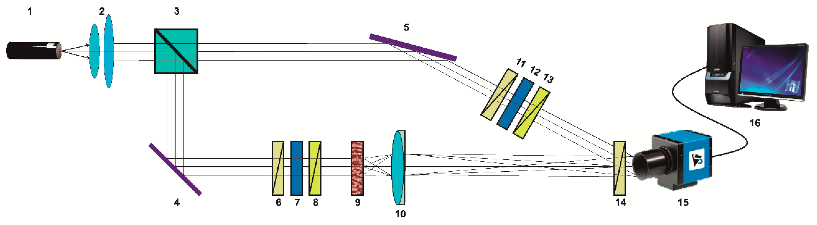
2.1. Optical Scheme and 3D Mueller-Matrix Polarimetry Technique

Figure 1 shows the optical setup for 3D Mueller-matrix polarimetry of biological layers [35,36,37,38].
The parallel ( Ø = 2 × 10 3   μ m ) laser beam (He-Ne laser 1, λ = 0.6328   μ m ) has been formed using collimator two. Further, a laser beam has been separated on two beams (“irradiating” and “reference”) using beam splitter three. The “irradiating” beam has been passed through the polarization filters six–eight using rotary mirror four. Further, this beam illuminated the sample of the biological layer nine.
The image of the object nine has been obtained using lens 10 (Nikon CFI Achromat P, focal length 30 mm, numerical aperture 0.1, and magnification 4×) and photosensitive pad ( m × n = 1280 × 960 pixels) of the digital camera 15.
The “reference” beam has been passed through the polarization filters 11–13 using mirror five. Further, this beam illuminated image plane of the object 9.
The resulting interference pattern passed through the polarizer-analyzer 14 has been recorded using digital camera 15 (The Imaging Source DMK 41AU02.AS, monochrome 1/2 “CCD, Sony ICX205AL (progressive scan), resolution—1280 × 960, the size of the light-sensitive pad—7600 × 6200 μm, sensitivity—0, 05 lx, dynamic range—8 bit, and SNR—9 bit).
The polarization states of the “irradiating” and “reference” beams have been formed by means of polarization filters six–eight and 11–13.
Each filter consists of:
  • “input” polarizers six and 11 forming plane-polarized beams with azimuth 0 ° ;
  • quarterwave plates seven and 12 (Achromatic True Zero-Order Waveplate) and polarizer four (B + W Kaesemann XS-Pro Polarizer MRC Nano) forming right-circularly polarized beams ;
  • “output” polarizers eight and 13, forming a series of plane-polarized beams 0 ° ; 90 ° ; 45 ° .
  • The procedure of determination of the layered distributions of diffuse tomograms DT red ( φ j ; x ; y ) includes the following steps:
  • Formation in the irradiating and reference laser beams the next polarization states— 0 ° ; 90 ° ; 45 ° ; .
  • Registration of each interference pattern through the polarizer-analyzer 14 with a consistent orientation of the plane of transmission at angles Ω = 0 ° ; Ω = 90 ° .
  • Application of Fourier transform procedure to interference pattern and using the inverse Fourier transform to obtaining the distributions of complex amplitudes U ( x , y ) = | U | ( x , y ) expi φ j in different phase planes ( φ j = 2 π λ r ; 0 r z ) of the object field with an arbitrary step Δ φ j = 0 q is realized [39,40].
  • In each phase plane φ j ( x ; y ) , for a series of planar (with azimuths 0 ° ; 90 ° ; 45 ° ) and the right of circularly ( ) polarized irradiating beams, the distributions of the four sets of parameters of the Stokes vector S i ( 0 ° : 90 ° ; 45 ° ; ) are calculated.
    S 1 0 0 ; 90 0 ; 45 0 ; φ J , x , y = U x 0 0 ; 90 0 ; 45 0 ; 2 + U y 0 0 ; 90 0 ; 45 0 ; 2 ; S 2 0 0 ; 90 0 ; 45 0 ; φ J , x , y = U x 0 0 ; 90 0 ; 45 0 ; 2 U y 0 0 ; 90 0 ; 45 0 ; 2 ; S 3 0 0 ; 90 0 ; 45 0 ; φ J , x , y = 2 Re U x 0 0 ; 90 0 ; 45 0 ; U y * 0 0 ; 90 0 ; 45 0 ; ; S 4 0 0 ; 90 0 ; 45 0 ; φ J , x , y = 2 Im U x 0 0 ; 90 0 ; 45 0 ; U y * 0 0 ; 90 0 ; 45 0 ; . .
  • On the basis of Equation (16) layered Muller-matrix images M i k ( φ j , x , y ) are determined as:
    M φ j , x , y = M 11 ; M 12 ; M 13 ; M 14 ; M 21 ; M 22 ; M 23 ; M 24 ; M 31 ; M 23 ; M 24 ; M 34 ; M 41 ; M 24 ; M 34 ; 44 φ j , x , y = = 0.5 S 1 0 + S 1 90 ; S 1 0 S 1 90 ; S 1 45 S 1 135 ; S 1 S 1 ; S 2 0 + S 2 90 ; S 2 0 S 2 90 ; S 2 45 S 2 135 ; S 2 S 2 ; S 3 0 + S 3 90 ; S 3 0 S 3 90 ; S 3 45 S 3 135 ; S 3 S 3 ; S 4 0 + S 4 90 ; S 4 0 S 4 90 ; S 4 45 S 4 135 ; S 4 S 4 φ j , x , y
Based on the set of distributions (17), a series of layer wise distributions of phase anisotropy M i k ( φ j ; x ; y ) 0.5 r 2 ( ln M 22 + ln M 33 + ln M 44 ) 1 { 1 ln M 22 ( B L ˜ 0 ; 90 ) ; ln M 33 ( B L ˜ 45 ; 135 ) ; ln M 44 ( B C ˜ ; ) } ( φ j ; x ; y ) is determined.

2.2. Samples

Blood from 18 healthy donors (group 1) and 18 patients with prostate cancer (group 2) were used in this study. Each sample film has been obtained by applying a drop of biological fluid to a substrate of optically homogeneous glass, followed by drying at room temperature. The optical thickness ( τ ) of the sample films varied within the range 0.68 τ 0.75 , the degree of depolarization Δ 41 % Δ 52 % .
Firstly, the functional possibility of optical anisotropy parameters 3D reproduction has been considered using the example of a polycrystalline blood film from healthy donor. Further, possibility of differentiation between polycrystalline whole blood films taken from healthy donors and patients with prostate cancer has been investigated.

3. Results and Discussion

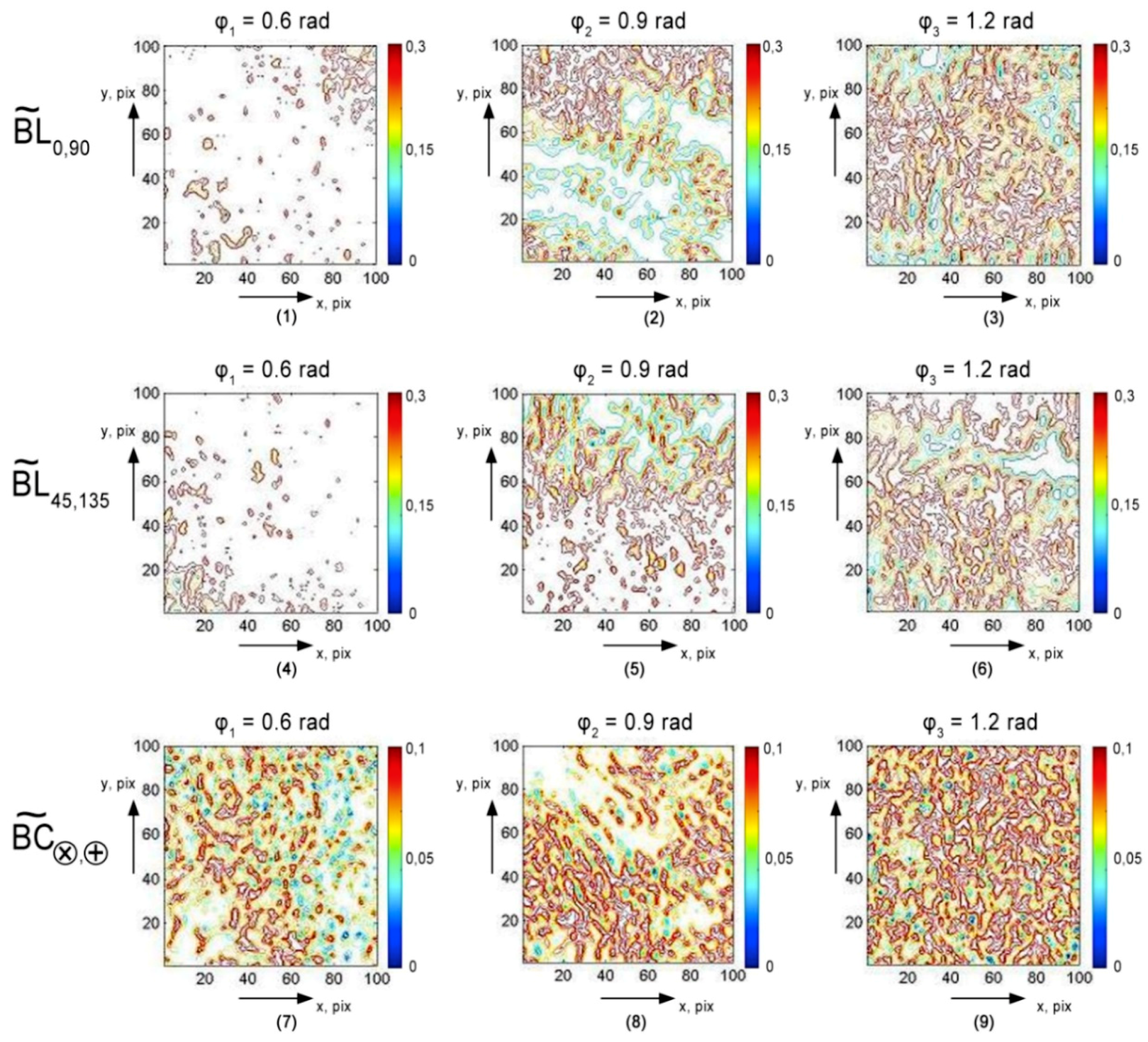
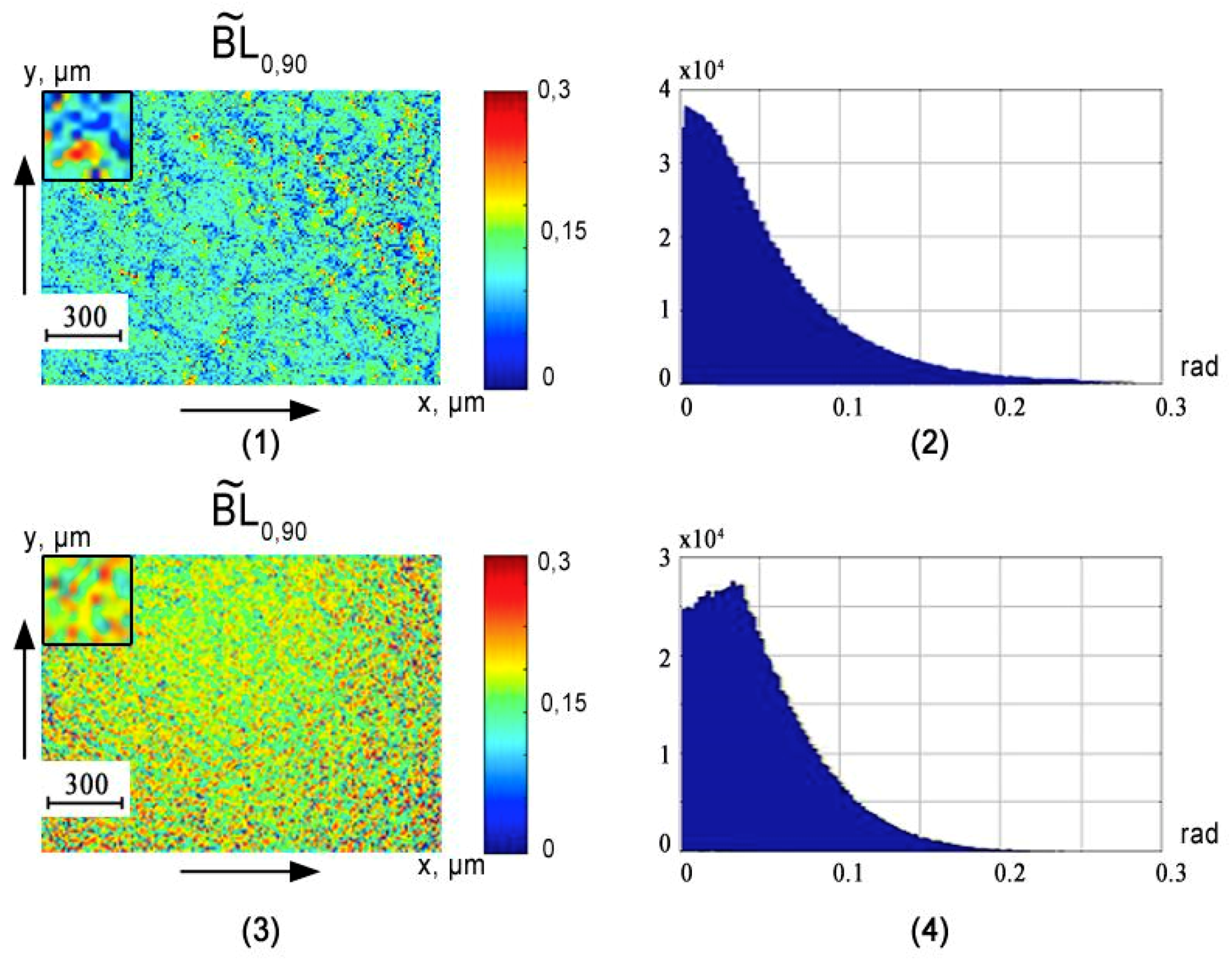
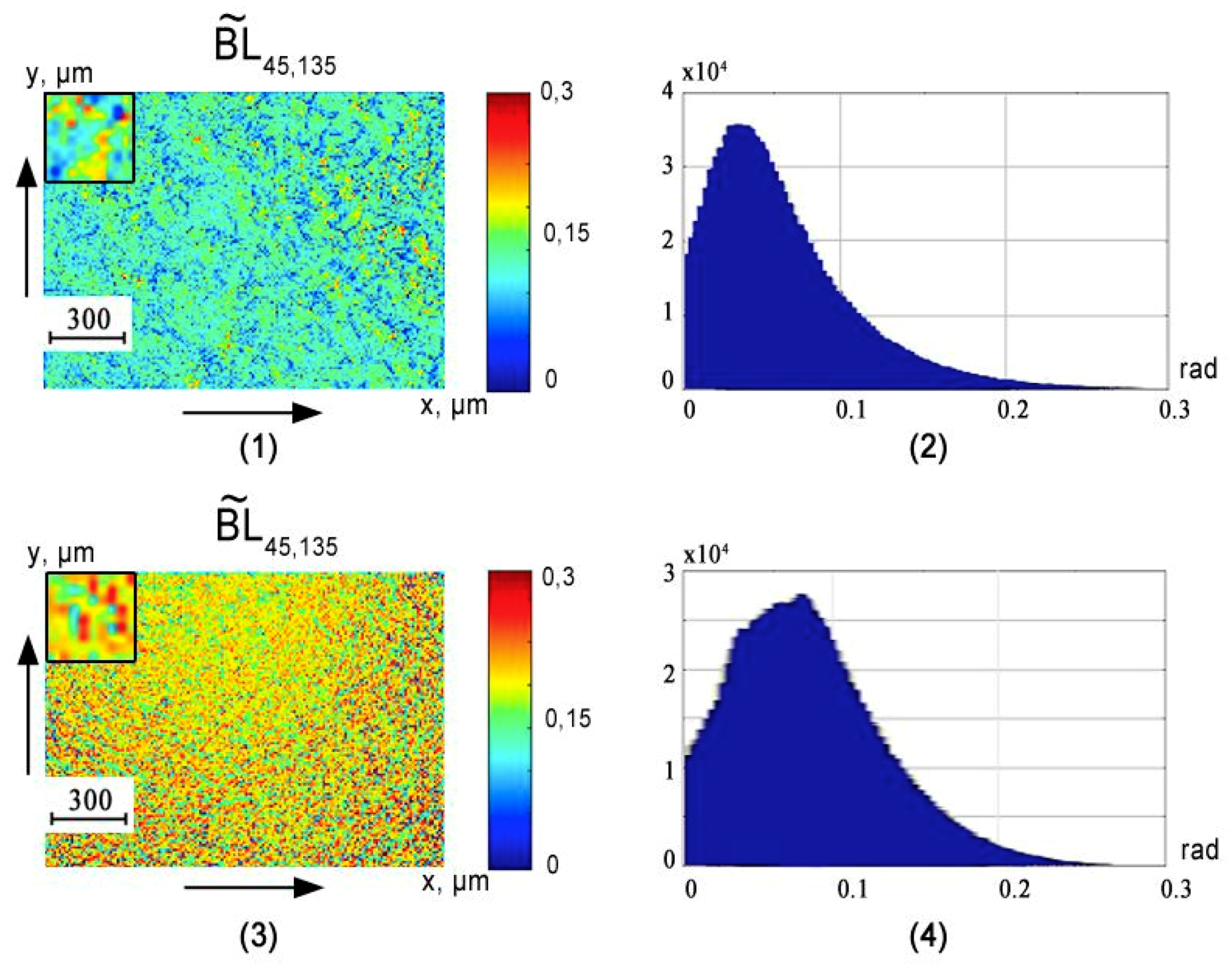
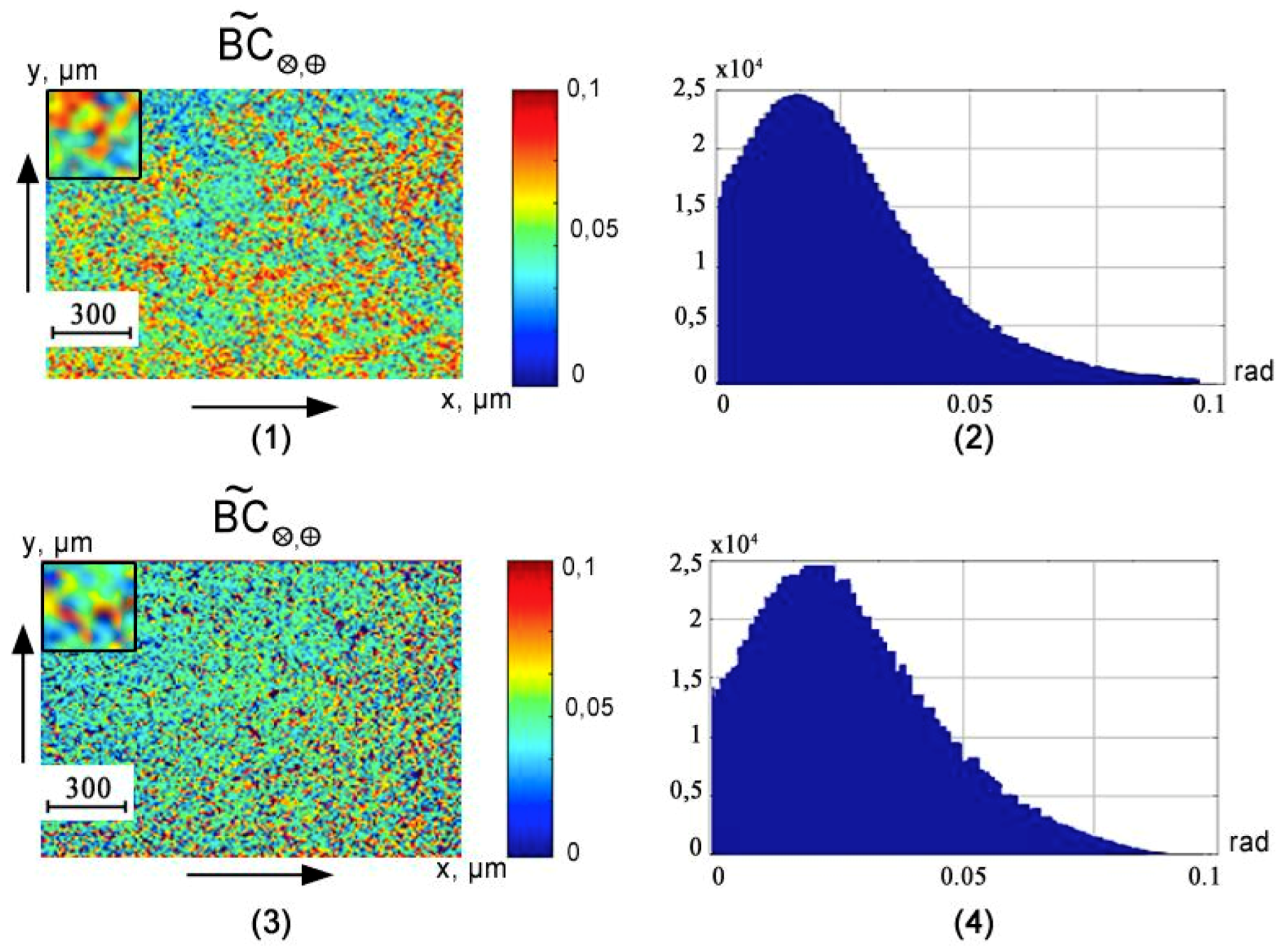
3.1. Layered Maps of Fluctuations in the Parameters of Phase Anisotropy of a Partially Depolarizing Polycrystalline Film of Blood

Figure 2 presents the diffuse tomograms DT red ( B L ˜ 0 ; 90 ) ((1)–(3)), DT red ( B L ˜ 45 ; 135 ) (4)–(6)), DT red ( B C ˜ ; ) (7)–(9)) in the phase sections φ 1 = 0.6 r a d ((1), (4), (7)), φ 2 = 0.9 r a d (2), (5), (8)), φ 1 = 1.2 r a d (3), (6), and (9)) fluctuations of linear and circular birefringence of a partially depolarizing polycrystalline blood film from healthy donor ( τ = 0.71 ; Δ = 46 % ).
Analysis of the diffuse tomograms DT red ( φ j , x , y ) of an optically anisotropic blood film, presented at Figure 2, revealed a good correlation between the experimental data (Equations (16) and (17)) and theoretical data (Equations (10)–(15)):
  • Individuality of layer wise coordinate distributions of linear ( ( B L ˜ 0 ; 90 ) ; ( B L ˜ 45 ; 135 ) ) and circular ( ( B C ˜ ; ) ) birefringence parameters (Figure 2) fluctuations;
  • Dependence of the structure DT red ( φ j ; x ; y ) on the value of the phase section φ j ;
  • Increasing ( ) of amplitude fluctuations DT red { ( B L ˜ 0 ; 90 ) ; ( B L ˜ 45 ; 135 ) ; ( B C ˜ ; ) } ( x , y ) with growing of φ j .
  • In each phase cross-section, the coordinate distributions DT red ( φ j ; x ; y ) were estimated by calculating the aggregate of statistical moments of the first–fourth order X i = 1 ; 2 ; 3 ; 4 [3,4,5]. By means of MATLAB software, we calculated the histograms (operator “hist”) and statistical moments of the first–fourth order (operator mean, STD, skewness, excess), which characterize the distributions DT red ( φ j ; x ; y )
    { X 1 = 1 K j = 1 K DT red ( φ j ; x ; y ) ; X 2 = 1 K j = 1 K ( DT red ( φ j ; x ; y ) X 1 ) j 2 ; X 3 = 1 X 2 3 1 K j = 1 K ( DT red ( φ j ; x ; y ) X 1 ) j 3 ; X 4 = 1 X 2 4 1 K j = 1 K ( DT red ( φ j ; x ; y ) X 1 ) j 4
Here, K is the number of pixels on the CCD-camera. These parameters characterize the mean value ( X 1 ), dispersion ( X 2 ), skewness ( X 3 ), and kurtosis or “peak sharpness” ( X 4 ) of the distributions DT red ( φ j ; x ; y ) .
Table 1 presents a series of “phase” dependences of the value X i = 1 ; 2 ; 3 ; 4 that characterize the distributions { DT red ( B L ˜ 0 ; 90 ) ; DT red ( B L ˜ 45 ; 135 ) ; DT red ( B C ˜ ; ) } ( x ; y ) of the polycrystalline blood film from healthy donors.
Analysis of the data presented in Table 1 revealed the following statistical scenario for the variation of the distribution of fluctuations in the parameters of optical anisotropy:
φ j { X 1 ; 2 ( DT red ( B L ˜ 0 ; 90 ; B L ˜ 45 ; 135 ; B C ˜ ; ) ) ; X 3 ; 4 ( DT red ( B L ˜ 0 ; 90 ; B L ˜ 45 ; 135 ; B C ˜ ; ) ) .
Such changes in magnitude X i = 1 ; 2 ; 3 ; 4 can be attributed to the change in the multiplicity of light scattering in the volume of a polycrystalline film of blood. In the region of small φ j distributions DT red ( B L ˜ 0 ; 90 ) ; DT red ( B L ˜ 45 ; 135 ) ; DT red ( B C ˜ ; ) , they are asymmetric ( X 3 ; 4 > X 1 ; 2 ) [3,4,5]. Due to the increase in multiplicity ( φ j ) according to the central boundary theorem [41], the structure of such distributions tends to be normal ( X 1 ; 2 ; X 3 ; 4 0 ).
The most sensitive to changes in the polarization manifestations of fluctuations in the phase anisotropy parameters of the polycrystalline blood film were statistical moments of the third and fourth orders (marked by * in Table 1). The range of their variations reaches:
  • DT red ( B L ˜ 0 ; 90 ) —1.77–1.81 times;
  • DT red ( B L ˜ 45 ; 135 ) —1.83–1.89 times;
  • DT red ( B C ˜ ; ) —1.81–2.82 times.

3.2. 3D Mueller-Matrix Differentiation of Diffuse Polycrystalline Films of Blood

Optical technology for differential diagnosis of depolarizing polycrystalline whole blood films from healthy donors (group 1) and patients with prostate cancer (group 2) includes:
  • Determination in each group of samples of a series of “phase” layered images of 3D distributions DT red { B L ˜ 0 ; 90 ; B L ˜ 45 ; 135 ; B C ˜ ; } ( φ 1 = 0.3 r a d ; 2 φ 1 ; , 6 φ 1 ) .
  • Calculations for each “phase” section φ j of the statistical moments of the first–fourth order X i = 1 ; 2 ; 3 ; 4 { DT red [ B L ˜ 0 ; 90 ; B L ˜ 45 ; 135 ; B C ˜ ; ] ( φ j , x , y ) } .
  • Definition of “phase” planes ( φ ), where the differences Δ X i = X i ( g r o u p 1 ) X i ( g r o u p 2 ) between the statistical moments are maximum—( Δ X i = 1 ; 2 ; 3 ; 4 Δ X i = 1 ; 2 ; 3 ; 4 ( φ ) max ).
  • In the phase plane φ , the mean Δ X ¯ i = 1 ; 2 ; 3 ; 4 and η ( Δ X i ) error within the polycrystalline blood films from group 1 and group 2 are determined.
  • For the possible clinical use of this method [42,43,44] for each of the statistical moments X i = 1 ; 2 ; 3 ; 4 ( φ ) —sensitivity ( R = a a + b 100 % ) specificity ( Q = c c + d 100 % ); balanced accuracy ( Ac = R + Q 2 ) [41,42,43] is calculated, where a and b are both the number of correct and incorrect diagnoses within group 2; c and d —the same within group 1.
Figure 3, Figure 4 and Figure 5 show the phase ( φ = 0.85 r a d ) cross sections ( Δ X i = 1 ; 2 ; 3 ; 4 Δ X i = 1 ; 2 ; 3 ; 4 ( φ ) max ) of 3D distributions of diffuse tomograms DT red ( B L ˜ 0 ; 90 ) (see Figure 3), DT red ( B L ˜ 45 ; 135 ) (see Figure 4), DT red ( B C ˜ ; ) (see Figure 5) of polycrystalline blood films from healthy donors (fragments (1) and (2)) and patients with prostate cancer (fragments (3) and (4)).
Table 2 shows the statistical analysis of the “phase” cross-sections φ = 0.85 r a d , as well as the level of balanced accuracy Ac , % .
A comparative analysis of the obtained data based on the statistical examination of the spatial distributions of magnitude of fluctuations in the linear and circular birefringence of polycrystalline blood films revealed a good ( 80 % Ac ( X 3 ; 4 ( B L ˜ 0 ; 90 ; 45 ; 135 ) ) 85 % ) and excellent ( Ac ( X 3 ; 4 ( B C ˜ ; ) ) 90 % ) level of balanced accuracy [42,43,44] in the differential diagnosis of oncological prostate pathology (marked by * in Table 2).
These results can be explained by the fact that the prevailing blood from patients with prostate cancer is the mechanisms [3,4,5,17,18,21,22,23,24,25,26,27]:
(1)
The growth of linear birefringence fluctuations ( B L ˜ 0 ; 90 ; B L ˜ 45 ; 135 ) due to the formation of supramolecular polycrystalline protein structures (albumin, fibrin);
(2)
Increasing concentration and crystallization of birefringent leukocytes;
(3)
The growth of circular birefringence fluctuations ( B C ˜ ; ) due to the increase in the concentration and crystallization of optically active globulin molecules.

4. Conclusions

The method of 3D Mueller-matrix diffuse tomography of distributions DT red { B L ˜ 0 ; 90 ; B L ˜ 45 ; 135 ; B C ˜ ; } ( φ 1 = 0.3 r a d ; 2 φ 1 ; , , 6 φ 1 ) of fluctuations in the parameters of linear and circular birefringence of partially depolarizing polycrystalline films of biological fluids has been theoretically substantiated and experimentally tested. The dynamics of the change in the magnitude of the statistical moments of the first–fourth orders characterizing layer-by-layer distributions of the fluctuations of the linear and circular birefringence of a polycrystalline film of blood of a healthy donor in different “phase” sections of its volume has been investigated and analyzed. The most sensitive to prostate cancer parameters are statistical moments of the third and fourth orders ( Δ X i = ; 3 ; 4 Δ X i = 3 ; 4 ( φ = 0.85 r a d ) max ), which characterize the distribution of fluctuations B L ˜ 0 ; 90 ; B L ˜ 45 ; 135 ; B C ˜ ; in the parameters of phase anisotropy of polycrystalline blood films of practically healthy donors and patients with prostate cancer. Respectively, good ( 80 % Ac ( X 3 ; 4 ( B L ˜ 0 ; 90 ; 45 ; 135 ) ) 85 % ) and excellent ( Ac ( X 3 ; 4 ( B C ˜ ; ) ) 90 % ) accuracy of the 3D Mueller-matrix tomography approach for differentiating samples of whole-blood polycrystalline films of healthy donors and patients with prostate cancer has been achieved.

Author Contributions

Manuscript preparation: V.U., A.Sd., A.D., A.U., I.M. Conceptualization: V.U., A.D., A.U., Y.U., I.M. Measurements, data processing V.U., A.Sd., A.D., O.V., M.G., M.S. Data curation, figures preparation: V.U., A.D., Y.U. Formal analysis: A.D., A.Sy., Y.U., V.U., A.U. Funding acquisition: Y.U., A.U., I.M. Investigation: A.D., A.Sy., I.M., Y.U., A.B. Methodology: A.D., Y.U., V.U., A.U. Project administration: Y.U., A.U., A.B., I.M.

Funding

Authors acknowledge financial support of the Academy of Finland (grant projects: 314369 and 311698). ASand IM would like to express sincere thanks to INFOTECH. IM acknowledges partial support from the MEPhI Academic Excellence Project (Contract No. 02.a03.21.0005), and National Research Tomsk State University Academic D.I. Mendeleev Fund Program.

Conflicts of Interest

The authors declare no conflict of interest.

References

  1. Manhas, S.; Swami, M.K.; Buddhiwant, P.; Ghosh, N.; Gupta, P.K.; Singh, K. Mueller matrix approach for determination of optical rotation in chiral turbid media in backscattering geometry. Opt. Exp. 2006, 14, 190–202. [Google Scholar] [CrossRef]
  2. Deng, Y.; Zeng, S.; Lu, Q.; Luo, Q. Characterization of backscattering Mueller matrix patterns of highly scattering media with triple scattering assumption. Opt. Exp. 2007, 15, 9672–9680. [Google Scholar] [CrossRef]
  3. Ushenko, A.G.; Pishak, V.P. Laser Polarimetry of Biological Tissue: Principles and Applications. In Handbook of Coherent-Domain Optical Methods: Biomedical Diagnostics, Environmental and Material Science; Tuchin, V.V., Ed.; Kluwer Academic Publishers: Boston, MA, USA, 2004; Volume I, pp. 93–138. [Google Scholar]
  4. Angelsky, O.V.; Ushenko, A.G.; Ushenko, Y.A.; Pishak, V.P.; Peresunko, A.P. Statistical, Correlation and Topological Approaches in Diagnostics of the Structure and Physiological State of Birefringent Biological Tissues. In Handbook of Photonics for Biomedical Science; Tuchin, V.V., Ed.; CRC Press Taylor & Francis Group: Boca Raton, FL, USA; London, UK; New York, NY, USA, 2010; pp. 283–322. [Google Scholar]
  5. Ushenko, Y.A.; Boychuk, T.M.; Bachynsky, V.T.; Mincer, O.P. Diagnostics of Structure and Physiological State of Birefringent Biological Tissues: Statistical, Correlation and Topological Approaches. In Handbook of Coherent-Domain Optical Methods; Springer Science + Business Media: New York, NY, USA, 2013; p. 107. [Google Scholar]
  6. Ghosh, N.; Wood, M.; Vitkin, A. Polarized light assessment of complex turbid media such as biological tissues via Mueller matrix decomposition. In Handbook of Photonics for Biomedical Science; Tuchin, V.V., Ed.; CRC Press, Taylor & Francis Group: London, UK, 2010; pp. 253–282. [Google Scholar]
  7. Swami, M.K.; Patel, H.S.; Gupta, P.K. Conversion of 3 × 3 Mueller matrix to 4 × 4 Mueller matrix for non-depolarizing samples. Opt. Commun. 2013, 286, 18–22. [Google Scholar] [CrossRef]
  8. Izotova, V.F.; Maksimova, I.L.; Nefedov, I.S.; Romanov, S.V. Investigation of Mueller matrices of anisotropic nonhomogeneous layers in application to an optical model of the cornea. Appl. Opt. 1997, 36, 164–169. [Google Scholar] [CrossRef] [PubMed]
  9. Borovkova, M.; Peyvasteh, M.; Ushenko, Y.O.; Dubolazov, O.V.; Ushenko, V.O.; Bykov, A.V.; Novikova, T.P.; Meglinski, I. Complementary analysis of Muller-matrix images of optically anisotropic highly scattering biological tissues. J. Eur. Opt. Soc. Rapid Publ. 2018, 14, 20. [Google Scholar] [CrossRef]
  10. Ushenko, V.A.; Dubolazov, A.V.; Pidkamin, L.Y.; Sakchnovsky, M.Y.; Bodnar, A.B.; Ushenko, Y.A.; Ushenko, A.G.; Bykov, A.; Meglinski, I. Mapping of polycristalline films of biological fluids utilizing Jones-matrix formalism. Laser Phys. 2018, 28, 025602. [Google Scholar] [CrossRef]
  11. Lu, S.Y.; Chipman, R.A. Interpretation of Mueller matrices based on polar decomposition. J. Opt. Soc. Am. A 1996, 13, 1106–1113. [Google Scholar] [CrossRef]
  12. Guo, Y.; Zeng, N.; He, H.; Yun, T.; Du, E.; Liao, R.; Ma, H. A study on forward scattering Mueller matrix decomposition in anisotropic medium. Opt. Exp. 2013, 21, 18361–18370. [Google Scholar] [CrossRef]
  13. Deboo, B.; Sasian, J.; Chipman, R.A. Degree of polarization surfaces and maps for analysis of depolarization. Opt. Exp. 2004, 12, 4941–4958. [Google Scholar] [CrossRef]
  14. Buscemi, I.C.; Guyot, S. Near real-time polarimetric imaging system. J. Biomed. Opt. 2013, 18, 116002. [Google Scholar] [CrossRef]
  15. Manhas, S.; Vizet, J.; Deby, S.; Vanel, J.C.; Boito, P.; Verdier, M.; Pagnoux, D. Demonstration of full 4? 4 Mueller polarimetry through an optical fiber for endoscopic applications. Opt. Exp. 2015, 23, 3047–3054. [Google Scholar] [CrossRef] [PubMed]
  16. Pierangelo, A.; Manhas, S.; Benali, A.; Fallet, C.; Totobenazara, J.L.; Antonelli, M.R.; Validire, P. Multispectral Mueller polarimetric imaging detecting residual cancer and cancer regression after neoadjuvant treatment for colorectal carcinomas. J. Biomed. Opt. 2013, 18, 046014. [Google Scholar] [CrossRef] [PubMed] [Green Version]
  17. Vladimir, Z.; Wang, J.B.; Yan, X.H. Human Blood Plasma Crystal and Molecular Biocolloid Textures—Dismetabolism and Genetic Breaches. Nat. Sci. J. Xiangtan Univ. 2001, 23, 118–127. [Google Scholar]
  18. Brutin, D.; Sobac, B.; Loquet, B.; Sampol, J. Pattern formation in drying drops of blood. J. Fluid Mech. 2011, 667, 85–95. [Google Scholar] [CrossRef] [Green Version]
  19. Ushenko, Y.A.; Ushenko, V.A.; Dubolazov, A.V.; Balanetskaya, V.O.; Zabolotna, N.I. Mueller-matrix diagnostics of optical properties of polycrystalline networks of human blood plasma. Opt. Spectrosc. 2012, 112, 884–892. [Google Scholar] [CrossRef]
  20. Ushenko, Y.A.; Dubolazov, A.V.; Balanetskaya, V.O.; Karachevtsev, A.O.; Ushenko, V.A. Wavelet-analysis of polarization maps of human blood plasma. Opt. Spectrosc. 2012, 113, 332–343. [Google Scholar] [CrossRef]
  21. Ungurian, V.P.; Ivashchuk, O.I.; Ushenko, V.O. Statistical analysis of polarizing maps of blood plasma laser images for the diagnostics of malignant formations. Proc. SPIE 2011, 8338, 83381L. [Google Scholar]
  22. Ushenko, V.A.; Dubolazov, O.V.; Karachevtsev, A.O. Two wavelength Mueller matrix reconstruction of blood plasma films polycrystalline structure in diagnostics of breast cancer. Appl. Opt. 2014, 53, B128–B139. [Google Scholar] [CrossRef]
  23. Prysyazhnyuk, V.P.; Ushenko, Y.A.; Dubolazov, A.V.; Ushenko, A.G.; Ushenko, V.A. Polarization-dependent laser autofluorescence of the polycrystalline networks of blood plasma films in the task of liver pathology differentiation. Appl. Opt. 2016, 55, B126–B132. [Google Scholar] [CrossRef]
  24. Ushenko, V.A.; Gavrylyak, M.S. Azimuthally invariant Mueller-matrix mapping of biological tissue in differential diagnosis of mechanisms protein molecules networks anisotropy. Proc. SPIE 2013, 8812, 88120Y. [Google Scholar]
  25. Ushenko, V.A.; Gorsky, M.P. Complex degree of mutual anisotropy of linear birefringence and optical activity of biological tissues in diagnostics of prostate cancer. Opt. Spectrosc. 2013, 115, 290–297. [Google Scholar] [CrossRef]
  26. Ushenko, V.A.; Dubolazov, A.V. Correlation and self similarity structure of polycrystalline network biological layers Mueller matrices images. Proc. SPIE 2013, 8856, 88562D. [Google Scholar]
  27. Ushenko, V.O. Spatial-frequency polarization phasometry of biological polycrystalline networks. Opt. Mem. Neur. Netw. 2013, 22, 56–64. [Google Scholar] [CrossRef]
  28. Ushenko, V.A.; Pavlyukovich, N.D.; Trifonyuk, L. Spatial-Frequency Azimuthally Stable Cartography of Biological Polycrystalline Networks. Int. J. Opt. 2013, 2013, 683174. [Google Scholar] [CrossRef]
  29. Acton, Q.A. Blood Cells—Advances in Research and Application—2012 Edition; Ashton, Q., Ed.; ScolarlyEditions™: Atlanta, GA, USA, 2012; p. 468. [Google Scholar]
  30. Drexler, W.; Fujimoto, J.G. Optical Coherence Tomography: Technology and Applications; Spriger Science & Business Media: New York, NY, USA, 2008; p. 1346. [Google Scholar]
  31. Ortega-Quijano, N.; Arce-Diego, J.L. Mueller matrix differential decomposition. Opt. Lett. 2011, 36, 1942–1944. [Google Scholar] [CrossRef] [PubMed]
  32. Ortega-Quijano, N.; Arce-Diego, J.L. Depolarizing differential Mueller matrices. Opt. Lett. 2011, 36, 2429–2431. [Google Scholar] [CrossRef] [PubMed]
  33. Ossikovski, R.; Devlaminck, V. General criterion for the physical realizability of the differential Mueller matrix. Opt. Lett. 2014, 39, 1216–1219. [Google Scholar] [CrossRef]
  34. Ossikovski, R.; Arteaga, O. Statistical meaning of the differential Mueller matrix of depolarizing homogeneous media. Opt. Lett. 2014, 39, 4470–4473. [Google Scholar] [CrossRef]
  35. Devlaminck, V.; Ossikovski, R. Uniqueness of the differential Mueller matrix of uniform homogeneous media. Opt. Lett. 2014, 39, 3149–3152. [Google Scholar] [CrossRef]
  36. Devlaminck, V. Physical model of differential Mueller matrix for depolarizing uniform media. J. Opt. Soc. Am. A 2013, 30, 2196–2204. [Google Scholar] [CrossRef]
  37. Dubolazov, O.V.; Ushenko, V.O.; Trifoniuk, L.; Ushenko, Y.O.; Zhytaryuk, V.G.; Prydiy, O.G.; Meglinski, I. Methods and means of 3D diffuse Mueller-matrix tomography of depolarizing optically anisotropic biological layers. Proc. SPIE 2017, 10396, 103962P. [Google Scholar]
  38. Ushenko, O.G.; Grytsyuk, M.; Ushenko, V.O.; Bodnar, G.B.; Vanchulyak, O.; Meglinski, I. Differential 3D Mueller-matrix mapping of optically anisotropic depolarizing biological layers. Proc. SPIE 2018, 10612, 106121I. [Google Scholar]
  39. Yasuno, Y.; Ju, M.; Hong, Y.; Makita, S.; Miura, M. In Vivo Three-Dimensional Investigation of Tissue Birefringence by Jones Matrix Tomography. In 2013 Conference on Lasers and Electro-Optics Pacific Rim; Paper WJ4_2; Optical Society of America: Washington, DC, USA, 2013. [Google Scholar]
  40. Kobata, T.; Nomura, T. Digital holographic three-dimensional Mueller matrix imaging. Appl. Opt. 2015, 54, 5591–5596. [Google Scholar] [CrossRef] [PubMed]
  41. Goodman, J.W. Statistical properties of laser speckle patterns. In Laser Speckle and Related Phenomena; Dainty, J.C., Ed.; Springer: Berlin, Gernamy, 1975; pp. 9–75. [Google Scholar]
  42. Cassidy, L.D. Basic concepts of statistical analysis for surgical research. J. Surg. Res. 2005, 128, 199–206. [Google Scholar] [CrossRef] [PubMed]
  43. Davis, C.S. Statistical Methods of the Analysis of Repeated Measurements; Springer: New York, NY, USA, 2002. [Google Scholar]
  44. Robinson, S.P. Principles of Forensic Medicine; Greenwich Medical Media: London, UK, 1996; p. 188. [Google Scholar]
Figure 1. Schematic presentation of experimental set-up of 3D Muller matrix tomography of biological layers. Here: 1—He-Ne laser; 2—collimator; 3—beam splitter; 4; 5—optical mirrors; 6; 8; 11; 13; 14—polarizers; 7; 12—quarter wave plates; 9—object of study; 10—strain-free microobjective; 15—digital camera; and 16—personal computer (PC) workstation.
Photonics 05 00054 g001
Figure 2. Diffuse tomograms DT red ( φ j ; 1000   μ m × 1000   μ m ) of linear and circular birefringence fluctuations of a polycrystalline blood film taken from healthy donors ( τ = 0.71 ; Δ = 46 % ). Further details are in the text.
Photonics 05 00054 g002
Figure 3. An example of maps and histograms of the DT red spatial distribution fluctuations of the linear birefringence ( B L ˜ 0 ; 90 ) of polycrystalline blood films taken from healthy donor ((1) and (2)) and cancer patient ((3) and (4)).
Photonics 05 00054 g003
Figure 4. An example of maps and histograms of the DT red spatial distribution fluctuations of the linear birefringence ( B L ˜ 45 ; 135 ) of polycrystalline blood films taken from healthy donor ((1) and (2)) and cancer patient ((3) and (4)).
Photonics 05 00054 g004
Figure 5. An example of maps and histograms of the DT red spatial distribution fluctuations of the circular birefringence ( B L ˜ ; ) of polycrystalline blood films taken from healthy donor ((1) and (2)) and cancer patient ((3) and (4)).
Photonics 05 00054 g005
Table 1. The statistical structure parameters of layered diffuse tomograms of the fluctuation phase anisotropy of a polycrystalline blood film from healthy donors.
DT red DT red ( B L ˜ 0 ; 90 ) DT red ( B L ˜ 45 ; 135 ) DT red ( B C ˜ ; )
φ j 0.6 rad0.9 rad1.2 rad0.6 rad0.9 rad1.2 rad0.6 rad0.9 rad1.2 rad
X 1 0.090.120.150.0550.0950.120.160.130.09
X 2 0.080.1050.130.0450.070.1050.130.110.08
X 3 0.38 *0.29 *0.21 *0.66 *0.52 *0.36 *0.31 *0.19 *0.11 *
X 4 0.32 *0.25 *0.18 *0.93 *0.78 *0.49 *0.38 *0.31 *0.21 *
* statistical moments the most sensitive to the polarization changes in the phase anisotropy parameters of the polycrystalline blood film.
Table 2. Efficiency of statistical analysis of diffuse tomograms of polycrystalline blood films for the differentiation between healthy donors and patients with prostate cancer patients.
DT red B L ˜ 0 ; 90 Ac , %
SamplesGroup 1Group 2
X 1 0.06 ± 0.00470.075 ± 0.006978
X 2 0.08 ± 0.00050.095 ± 0.00674
X 3 0.46 ± 0.022 *0.33 ± 0.018 *84
X 4 0.39 ± 0.019 *0.27 ± 0.015 *80
DT red B L ˜ 45 ; 135 Ac , %
SamplesGroup 1Group 2
X 1 0.07 ± 0.0040.09 ± 0.00574
X 2 0.105 ± 0.0030.12 ± 0.004576
X 3 0.76 ± 0.041 *0.59 ± 0.032 *84
X 4 1.03 ± 0.053 *0.81 ± 0.039 *82
DT red B C ˜ ; Ac , %
SamplesGroup 1Group 2
X 1 0.02 ± 0.0080.03 ± 0.0182
X 2 0.03 ± 0.0050.04 ± 0.00778
X 3 0.36 ± 0.019 *0.21 ± 0.011 *92
X 4 0.49 ± 0.024 *0.33 ± 0.017 *90
* ‘good’ and ‘excellent’ level of balanced accuracy, obtained based on the statistical examination of the spatial distributions of the magnitude of fluctuations observed in the maps of linear and circular birefringence of polycrystalline blood films (see further details in the text).

