Fourier Single-Pixel Imaging Based on Online Modulation Pattern Binarization

Abstract

Down-sampling Fourier single-pixel imaging is typically achieved by truncating the Fourier spectrum, where exclusively the low-frequency Fourier coefficients are extracted while discarding the high-frequency components. However, the truncation of the Fourier spectrum can lead to an undesired ringing effect in the reconstructed result. Moreover, the original Fourier single-pixel imaging necessitated grayscale Fourier basis patterns for illumination. This requirement limits imaging speed because digital micromirror devices (DMDs) generate grayscale patterns at a lower refresh rate. In order to solve the above problem, a fast and high-quality Fourier single-pixel imaging reconstruction method is proposed in the paper. In the method, the threshold binarization of the Fourier base pattern is performed online to improve the DMD refresh rate, and the reconstruction quality of Fourier single-pixel imaging at a low-sampling rate is improved by generating an adversarial network. This method enables fast reconstruction of target images with higher quality despite low-sampling rates. Compared with conventional Fourier single-pixel imaging, numerical simulation and experimentation demonstrate the effectiveness of the proposed method. Notably, this method is particularly significant for fast Fourier single-pixel imaging applications.

1. Introduction

Single-pixel imaging is a computational imaging method that enables image acquisition and capture using a single-pixel detector without the use of an array sensor [1,2,3]. Compared with array sensors, the benefits of a single-pixel detector are its quick reaction time, excellent sensitivity, and wide operating band [2]. Therefore, single-pixel imaging has attracted wide attention and has been used in terahertz imaging [4,5], 3D imaging [6,7], multispectral imaging [8,9], image encryption [10], target tracking [11,12,13], polarization imaging [14,15], underwater imaging [16,17], remote sensing [18,19], and other fields.

However, single-pixel detectors do not have spatial resolution capability. For single-pixel imaging, spatial light modulation and spatial information encoding-decoding methods are critical. Specifically, encoding refers to the use of a spatial light modulator to modulate the laser’s spatial distribution using different patterns decoding refers to obtaining the reconstructed result with the reconstruction algorithm. To improve the performance of single-pixel imaging, Fourier single-pixel imaging and single-pixel imaging with Gao–Boole patterns [20] have been sequentially proposed. These techniques aim to improve the quality of target image reconstruction in single-pixel imaging by using deterministic patterns instead of random patterns. The quality of image reconstruction is substantially enhanced by Fourier single-pixel imaging (FSPI) [21,22,23,24,25], which employs the Fourier basis patterns for spatial light modulation to obtain the Fourier spectrum of the target. The quality and efficiency of image reconstruction are both important for FSPI. However, numerous single-pixel measurements result in a longer data gathering process, which slows down imaging speed. Digital micromirror devices that modulate grayscale patterns have a low-refresh rate, and the Fourier single-pixel imaging method based on grayscale patterns in lighting is likewise constrained by the imaging speed.

In order to achieve fast speed and high-quality imaging results at a low-sampling rate, fast Fourier single-pixel imaging via a generative adversarial network (F2SPI-GAN) is proposed in the paper. The method consists of two parts: Fourier basis patterns, binarization, and reconstruction. In the paper, the online modulation of grayscale Fourier base pattern binarization is adopted. Binarization Fourier basis patterns are obtained by binarizing the fixed threshold value of the grayscale Fourier basis patterns. The purpose of online modulation binarization is to save DMD memory and improve system performance and program stability. The decoding results are reconstructed by the generative adversarial network based on deep learning. The use of this method effectively reduces the ringing impact of the rebuilt results and ensures that high-quality results may be quickly recreated with a low-sampling rate. The generator of F2SPI-GAN uses an improved encoder and decoder as the primary network architecture. The network has a double-skip connection in between the encoding layer and the decoding layer, while one of the skip connections has an attention block added to it to enhance the network’s ability to be reconstructed. The choice of using a convolutional neural network as the discriminator is to guide and supervise the image generation process of the generator in the proposed method. The input of the generator is the under-sampled image obtained by projecting the binarized Fourier basis patterns, and the output is the reconstructed image. Numerical simulation and experimental consequences show that the image reconstructed by the F2SPI-GAN method has higher quality, higher generation ability, and fast speed imaging efficiency. The proposed F2SPI-GAN is applicable for fast, high-quality imaging at low-sampling rates.

In general, the contribution of this study is mainly in three aspects:

(1)

The binarization Fourier basis pattern is used to replace the grayscale Fourier basis patterns to improve the modulation speed of DMD and realize fast Fourier single-pixel imaging.

(2)

The F2SPI-GAN method is proposed to obtain high-quality reconstruction results, in which the generator adopts double-skip connections between corresponding layers and adds an attention block to each skip connection.

(3)

Numerical simulation and experimentation demonstrate the effectiveness of the proposed method. The F2SPI-GAN method can achieve fast and high-quality imaging at a low-sampling rate. This work speeds up the application process for Fourier single-pixel imaging.

2. Related Work

2.1. The Method of Fourier Basis Pattern Binarization

To enhance Fourier single-pixel imaging effectiveness, researchers proposed spectrum under-sampling [26] and Fourier basis pattern binarization [27,28,29] to improve the speed of FSPI. Spatial frequency under-sampling in FSPI refers to acquiring only the low-frequency component and discarding the high-frequency component. Fourier basis pattern binarization refers to converting grayscale patterns into binarization pattern illumination, which is mainly divided into the following three methods: spatial dithering strategy [27], signal dithering strategy [28], and improved error diffusion jitter algorithm [29].

The spatial jitter strategy is based on upsampling and error diffusion jitter to binarize the Fourier basis patterns. The process of upsampling is necessary because it can introduce additional pixels into the pattern and therefore eliminate quantization errors due to dithering to some extent. Imaging spatial resolution is sacrificed because additional physical pixels are required to represent pattern pixels. Under their 20,000 Hz DMD projection rate of 10 frames per second, they capture a dynamic scene of 256 × 256 pixels. To a certain extent, it speeds up the image acquisition speed of FSPI. However, the spatial jitter algorithm comes at the expense of spatial resolution. In addition, generating high-resolution images causes the DMD to load the Fourier basis pattern and occupy more memory.

The signal dithering strategy is a technique aimed at enhancing the imaging efficiency of FSPI by employing a detected signal that is computationally weighted through binary pattern illumination using a DMD. Using DMD at a projected rate of 22 KHz, 9 frames per second capture a 128 × 128 pixel dynamic scene. Compared with the spatial dithering strategy, this method can improve the speed of DMD-based Fourier single-pixel imaging without sacrificing spatial resolution. The technology based on the signal jitter algorithm involves a balance between temporal resolution and spatial resolution but still cannot meet the high-speed and high-resolution imaging requirements.

The improved error diffusion jitter algorithm method uses two sets of binarized Fourier basis patterns for spatial light modulation. Each set of patterns is determined by using a different scanning strategy without upsampling. The two images are synthesized to even out the noise caused by the dithering. The method can therefore reconstruct a high-quality, full-resolution, and full-FOV image. For the improved error diffusion dithering algorithm, although it can satisfy full resolution and high-quality fast Fourier single-pixel imaging, it is still difficult to reconstruct high-quality images at a low-sampling rate.

2.2. Reconstruction Network

The researchers proposed Fourier single-pixel imaging based on deep learning to further enhance the reconstruction quality at a low-sampling rate. Deep convolutional autoencoder networks and generative adversarial networks are two instances of Fourier single-pixel imaging based on deep learning [25,30].

The deep convolutional autoencoder network is a type of neural network architecture used for unsupervised learning and image reconstruction tasks. It consists of two main parts: an encoder and a decoder. The deep convolutional autoencoder network learns end-to-end between the under-sampled image and the real image through symmetric skip connections. However, it cannot meet the requirements of larger resolution and faster imaging speed.

Drawing inspiration from the generative adversarial network, researchers introduced an approach called Fourier single-pixel imaging via the generative adversarial network. This model incorporates perceptual loss, pixel loss, and frequency loss into the total loss function, which effectively preserves intricate details in the target image. Consequently, the proposed model can achieve high-quality target image reconstruction directly from the FSPI measurements. By leveraging this innovative model, high-quality FSPI reconstruction results can be obtained even under low-sampling rate conditions. Although this method has achieved good results, the network model parameters of the architecture are too large. When deploying models, long inference times and large memory usage can lead to failure to meet the response requirements.

In order to enhance the imaging quality and imaging speed of Fourier single-pixel imaging, researchers have conducted related research and promoted the development of Fourier single-pixel imaging technology. However, it is still difficult to reconstruct high-quality images at high speed with a low-sampling rate. Therefore, one of the issues that has to be conquered is the speedy reconstruction of images of excellent quality at low-sampling rates.

3. Method

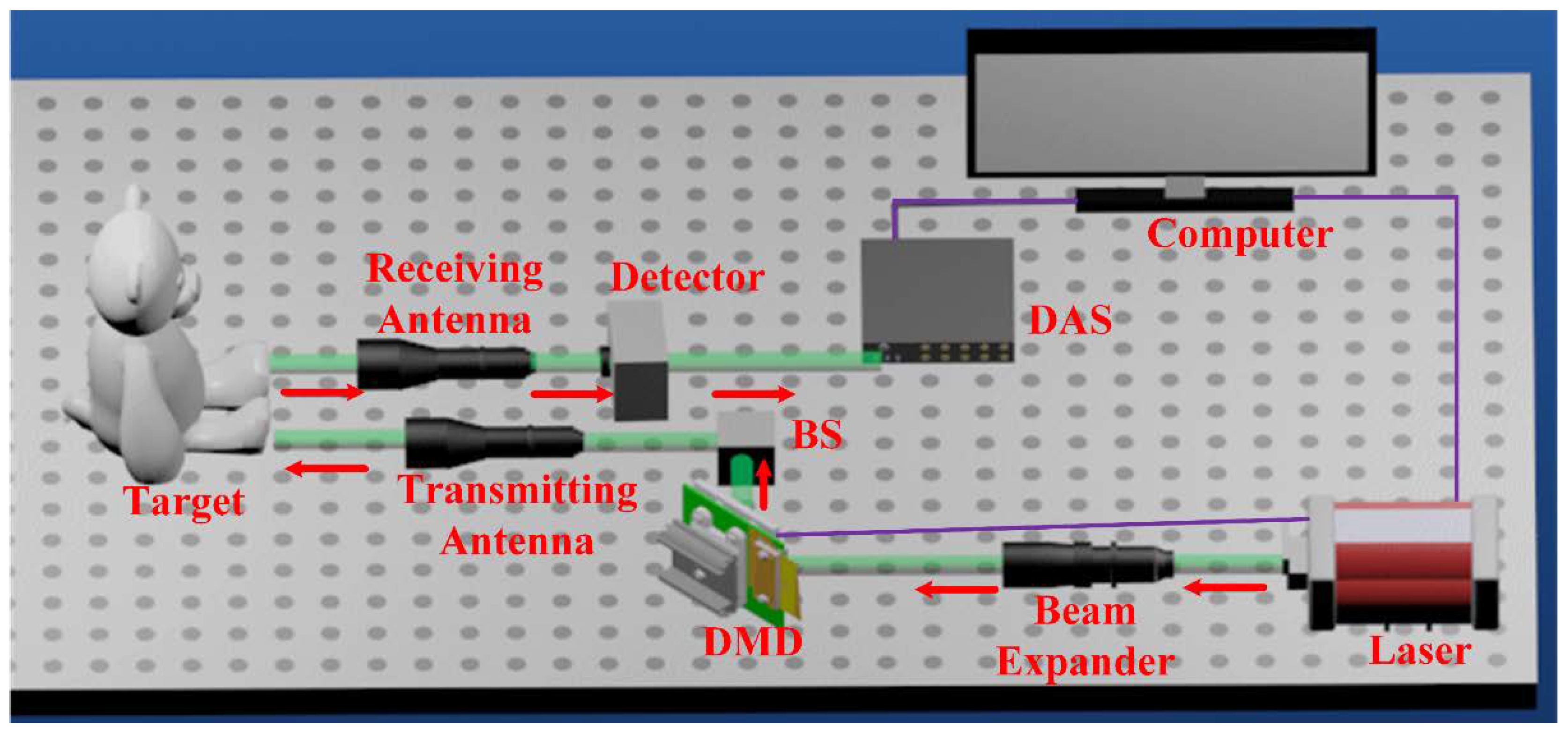
3.1. Forward Imaging Model

Figure 1 illustrates the schematic diagram of the Fourier single-pixel imaging system. The laser beam emits light, which is then expanded by the beam expander. Then, the spatial distribution of the light is modulated by the spatial light modulator according to the computer-controlled binarization Fourier basis patterns. The DMD-modulated laser passes through a 50–50% beam splitter (BS), altering its path, and then goes through the transmitting antenna to illuminate the target scene. The receiving antenna gathers and concentrates the illumination that is reflected from the target scene onto the single-pixel detector. The entire light intensity is measured by the data acquisition system (DAS), which then uses a USB connection to send the data to the computer for image reconstruction.

In conventional FSPI, grayscale Fourier basis patterns are employed for illumination, with each pattern being sinusoidal. These grayscale Fourier basis patterns can be represented by their spatial frequency (f_x, f_y) and initial phase φ:

$$P_{\phi }(x,y)=\frac{1}{2}+\frac{1}{2}·\cos \left(2\pi f_{x}x+2\pi f_{y}y+\phi \right)$$

(1)

Among them, the two-dimensional Cartesian coordinates are represented by x and y, while f_x and f_y correspond to the spatial frequencies along the x and y axes, respectively. φ is phase. To streamline the derivation process, it is assumed that the light intensity of the laser illumination on the modulator is uniform and is represented by S₀. The modulated laser is illuminated on the target object, and its distribution is denoted by S(x,y).

$$S\left(x,y\right)=P_{\phi }\left(x,y\right)S_0$$

(2)

After the Fourier basis pattern is irradiated on the target object, the optical signal intensity is detected by the single-pixel detector. The measured light intensity value of the single-pixel detector is expressed as:

$$Z_{\phi }\left(f_x,f_y\right)=Z_n+v{\displaystyle \iint U\left(x,y\right)S\left(x,y\right)}dxdy$$

(3)

Z_n represents the noise term. U(x,y) is the reflectance of the object. The factor v is associated with the magnification of the single-pixel detector. Spatial frequencies of (f_x, f_y) and beginning phases of 0, π/2, π, and 3π/2 are irradiated on the target object in accordance with the four-step phase-shifting methodology to get the Fourier spectrum T(f_x, f_y) corresponding to the spatial frequency of (f_x, f_y). Therefore, the single-pixel detector can measure 4 light intensity values D₀, D_π/2, D_π, and D_3π/2 at each spatial frequency. Fourier spectrum T(f_x, f_y) with frequency (f_x, f_y) can be calculated as follows:

$$T(f_x,f_y)=\left[Z_0(f_x,f_y)-Z_{\pi }(f_x,f_y)\right]+j\left[Z_{\pi /2}(f_x,f_y)-Z_{3\pi /2}(f_x,f_y)\right]=v·F\left\{R\left(x,y\right)\right\}$$

(4)

Here j represents an imaginary unit, and F{R(x,y)} denotes the Fourier transform of R(x,y). By performing an inverse Fourier transform on the equation mentioned above, the image of the reflective object can be reconstructed.

In order to speed up imaging, the paper adopts a binary pattern to approximate grayscale pattern lighting, which can be expressed as:

$$B_{\phi }\left(x,y\right)=\alpha +\frac{2}{\pi }{\displaystyle \sum _{n=1}^{\infty }\frac{\sin \left(\alpha n\pi \right)}{n}}\cos \left(n\left(2\pi f_{x}x+2\pi f_{y}y\right)+\phi \right)$$

(5)

Here α is impact factors and threshold values. The value of a is 0 to 1. As a result, the binary pattern distribution S(x,y) illuminating the target object can be expressed as:

$$S^{\prime }\left(x,y\right)=B_{\phi }\left(x,y\right)S_0$$

(6)

After the binarization Fourier basis pattern is irradiated on the target object, the optical signal intensity is detected by the single-pixel detector. The measured light intensity value of the single-pixel detector is expressed as:

$${Z^{\prime }}_{\phi }\left(f_x,f_y\right)=Z_n+v{\displaystyle \iint U\left(x,y\right)S^{\prime }\left(x,y\right)}dxdy$$

(7)

Therefore, the single-pixel detector can measure 4 light intensity values D₀, D_π/2, D_π, and D_3π/2 at each spatial frequency. Fourier spectrum T(f_x, f_y) with frequency (f_x, f_y) can be calculated as follows:

$$T^{\prime }(f_x,f_y)=\left[{Z^{\prime }}_0\left(f_x,f_y\right)-{Z^{\prime }}_{\pi }\left(f_x,f_y\right)\right]+j\left[{Z^{\prime }}_{\pi /2}\left(f_x,f_y\right)-{Z^{\prime }}_{3\pi /2}\left(f_x,f_y\right)\right]$$

(8)

where j is an imaginary unit. By substituting the four light intensity values into Equation (9), we can further simplify it and obtain the expression for T(f_x, f_y):

$$T^{\prime }(f_x,f_y)=\frac{4}{\pi }·v·\sin \left(\alpha \pi \right)·F\left\{R\left(x,y\right)\right\}+\frac{1}{{\left(f_x{f}_y\right)}^2}F\left\{R^{*}\left(0,0\right)\right\}{\displaystyle \sum _{n=2}^{\infty }\frac{\sin \left(\alpha n\pi \right)}{n\pi }}$$

(9)

In order to reduce the influence of binarization Fourier basis patterns on imaging quality, the result derived from Equation (9) should be close to Equation (4). Because the second term of Equation (9) is an unavoidable error term. Therefore, the previous term of Equation (9) is approximated by Equation (4). Because the gray Fourier base pattern is normalized, the threshold is selected in the range (0, 1), and the α value is calculated as 0.29 or 0.71.

Due to the conjugate symmetry of the Fourier spectrum, there is no need to sample the symmetry coefficients. According to conjugate symmetry, it takes 2 × M × N measurements to fully sample an object image with M × N pixels. However, for fast Fourier single-pixel imaging, full sampling requires a large number of measurements, and longer data acquisition times cannot meet the requirements of efficient imaging. Because the circle sampling strategy [25] has achieved good results, the system adopts the circle sampling strategy with a 1~3% sampling rate. However, when the sampling rate is low, the resulting image may lose detailed parts of the image and have a significant ringing effect. The use of binarization Fourier basis patterns instead of grayscale Fourier basis patterns will also reduce the quality of the image. In order to achieve fast and high-quality imaging at a low-sampling rate, it is necessary to reconstruct the under-sampling intensity image of the target scene using a reconstruction algorithm. After further reconstruction processing, a high-quality reconstructed image is finally obtained.

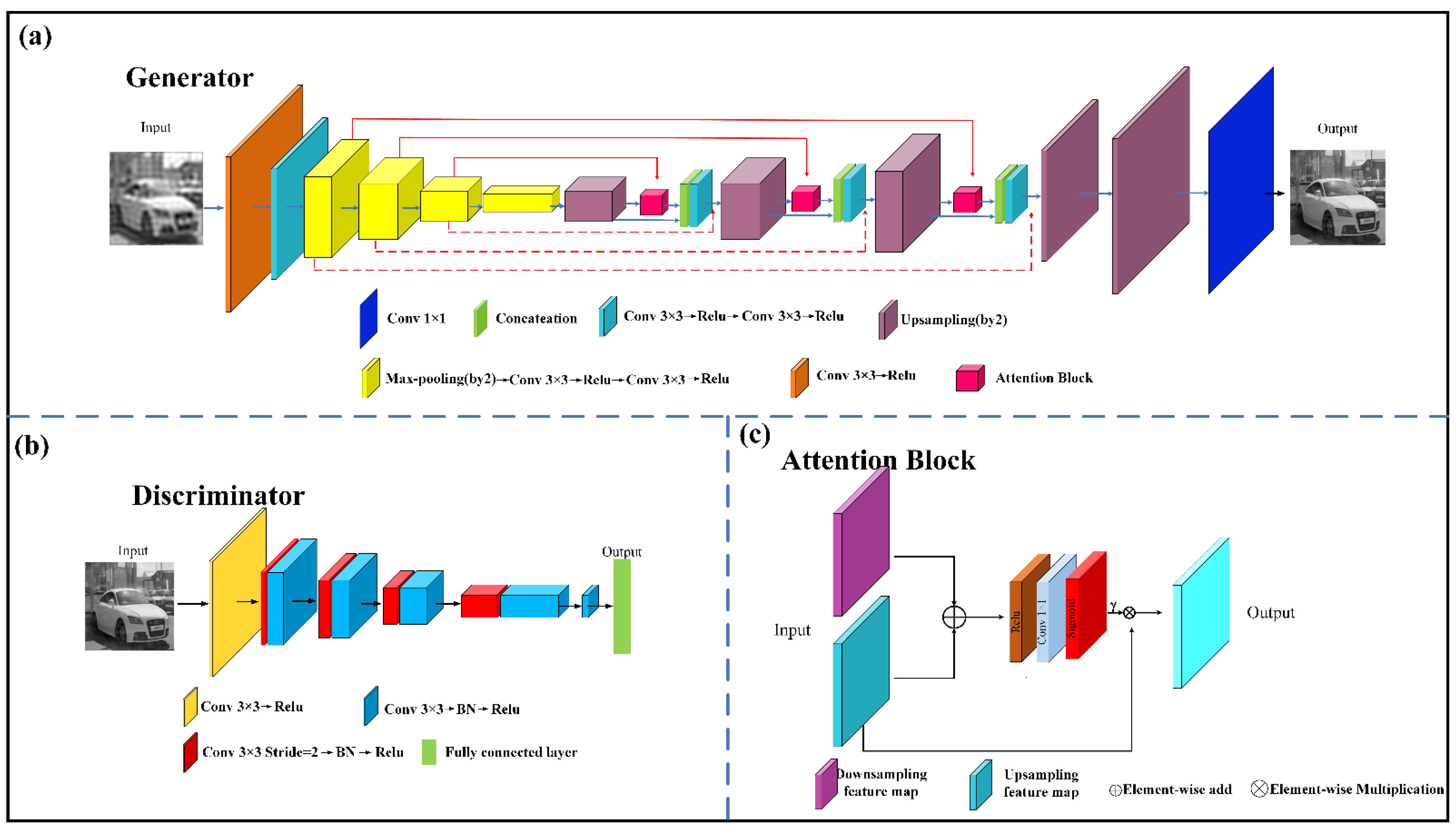
3.2. Network Architecture

The network architecture, denoted as F2SPI-GAN, is illustrated in Figure 2. The network comprises two main parts: the generator network G and the discriminator network D. The primary objective of the generator network G is to produce an image that closely resembles the real image, while the discriminator network D aims to distinguish between generated images and real images.

Generator: The proposed generator in Figure 2a is inspired by an encoder-decoder [30,31,32,33] structure. The input to the generator is an under-sampled image with a resolution of 256 × 256 and a number of channels of 1. The main function of the encoder is to extract image features, and the main function of the decoder is to recover the feature image. Among them, the encoder extracts the feature, structure, and content information of under-sampled images by using convolutional layers. The encoder consists of 6 2D convolution layers and 4 max-pooling layers. Each convolutional layer is followed by a ReLU activation function. The max-pooling layer is used to remove redundant information and simplify network complexity. After down-sampling by the encoder, a feature map with 2048 channels and a resolution of 4 × 4 is obtained. However, as the network layers deepen, some characteristics and details of the input signal may be lost. To address this issue, a skip connection is introduced in the reconstructed network. Unlike conventional skip connections, an attention block is incorporated into the skip connection path to filter noise and retain important features. The decoder obtains a 32-channel feature map with 256 × 256 resolution by upsampling. The final output is obtained by applying a 2D convolution with a kernel size of 1 × 1 and a stride of 1 to the feature map. Furthermore, to enhance the recovery of details, a skip connection path [33] is introduced, connecting the corresponding layers of the encoder and decoder. This double-skip connection facilitates the smooth flow of information between the encoder and decoder, leading to improved reconstruction results.

Discriminator: The structure of the discriminator is shown in Figure 2b. The role of the discriminator is to improve the reconstruction performance of the generator. The discriminator is composed of 9 2D convolutional layers, 4 batch normalization layers, and one fully connected layer. Among them, convolutional layers are used to extract features. The batch normalization layer accelerates convergence, improves stability, and acts as a form of regularization in deep neural networks. The fully connected layer converts the output of the 9 convolutional layers into a one-dimensional feature vector output. In this way, it is easy to achieve the purpose of discrimination.

Attention Block: Figure 2c shows the structure diagram of the attention block. Here, the two corresponding inputs correspond to the down-sampling layer of the encoder and the up-sampling layer of the decoder, respectively. The two are added pixel by pixel, followed by the ReLU activation function and 1 × 1 convolution, and then the attention coefficient γ is calculated by the sigmoid activation function. Then, multiply with the up-sampling layer of the decoder to obtain the output. Because the fine-grained information in the encoder is relatively large, a lot of it is redundant and unnecessary. The attention block is equivalent to filtering the current layer of the encoder, suppressing irrelevant information in the image, and highlighting the local medium-important features.

Double-skip connections: The double-skip connections consist of two connections: the concatenation connection and the element-wise add connection.

• Concatenation Connection: The introduction of concatenation connections serves two primary objectives. Firstly, as the network’s depth increases, there is a risk of losing intricate image details, which might not be easily recoverable through the deconvolution process alone. The feature maps transferred via the concatenation connections hold valuable detail information that aids the deconvolution process in producing more accurate and clear reconstructions. Secondly, when employing gradient-based backpropagation during training, the concatenation connections contribute to smoother and more efficient training dynamics. This promotes better convergence and improved training stability.
• Element-wise Add Connection: The integration of element-wise addition connections proves highly beneficial, particularly due to the important analogous characteristics shared by the input and output layers. This configuration results in a discernible enhancement in performance compared to a similar network lacking element-wise added connections. Furthermore, these connections effectively mitigate the vanishing gradient problem that can arise during training, leading to a more effective optimization process and improved overall training performance.

3.3. Loss Function of F2SPI-GAN

The loss function is used to measure the difference between the original image and the network reconstructed image. To enhance performance, the total loss function of the generator during training is determined by the weighted sum of perceptual loss, pixel loss, and adversarial loss. The perceptual loss is computed based on the VGG19 [34] network, which serves as a pre-trained network model. The perceptual loss is described as follows:

$$L_{percepyual}={\Vert f_{vgg19}(q_g)-f_{vgg19}(q)\Vert }_2^2$$

(10)

The pixel loss is described as follows:

$$L_{piexl}={\Vert q_g-q\Vert }_2^2$$

(11)

q_g represents the reconstruction image obtained from the network, while q denotes the target image. In addition, f_vgg19 is the network trained by VGG19.

The adversarial loss is expressed as follows:

$$L_{adversarial}=E_{i\sim P_i(i)}\left\{\log \left[D(G(i))\right]\right\}$$

(12)

In the equation, E represents the expected value of the distribution function, i denotes the input of the network model, P_i(i) represents the data distribution of i, and G(i) represents the output of the generator. Therefore, the total loss can be expressed as follows:

$$L_{total}=\mu L_{Lperceptual}+\nu L_{Lpixel}+\omega L_{Ladversarial}$$

(13)

In the proposed network model, the values of μ, ν, and ω are 0.006, 1, and 0.001, respectively. The optimizer employs Adam to optimize the loss function. The proposed network model is implemented on an RTX 3090 GPU (NVIDIA Corporation, Santa Clara, California, United States) using Tensorflow version 1.15.

Specifically, the weighting coefficient ν for L_pixel is set to 1, reflecting its critical role in guiding the network model to accurately reconstruct images based on pixel-level information. On the other hand, the loss functions L_perceptual and L_adversarial are assigned complementary weighting coefficients μ and ω, respectively, to control their impact on the training process. The values of μ and ω are chosen as 0.006 and 0.001, respectively. These coefficients strike a balance between leveraging perceptual information and incorporating adversarial training while maintaining the primary focus on pixel-level accuracy.

4. Numerical Simulations and Experimental Results

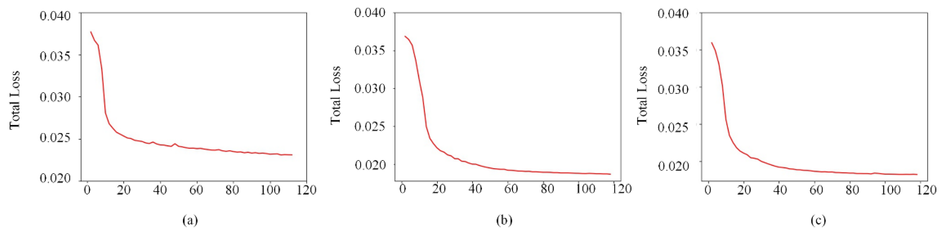
4.1. Dataset Preparation and Training Process

The training process utilizes a dataset of car images [35], which includes 196 classes of cars with a total of 16,185 images. From this dataset, 13,185 images are randomly selected to form the training set, while the remaining 3000 images constitute the testing set. Each image in the dataset has dimensions of 256 × 256 pixels.

The sampling rates represented by a, b, and c in Figure 3 are 1%, 2%, and 3%, respectively. Figure 3a depicts the loss curve using a sampling rate of 1%, while Figure 3b illustrates the loss curve employing a sampling rate of 2%. Additionally, Figure 3c portrays the loss curve with a sampling rate of 3%. As the number of epochs increases, the total loss function steadily decreases. Moreover, a higher sampling rate leads to a more rapid decline in the loss function. When the number of epochs exceeds 70, the loss function curve stabilizes, indicating that the network has converged to an optimal state, fulfilling the training objectives.

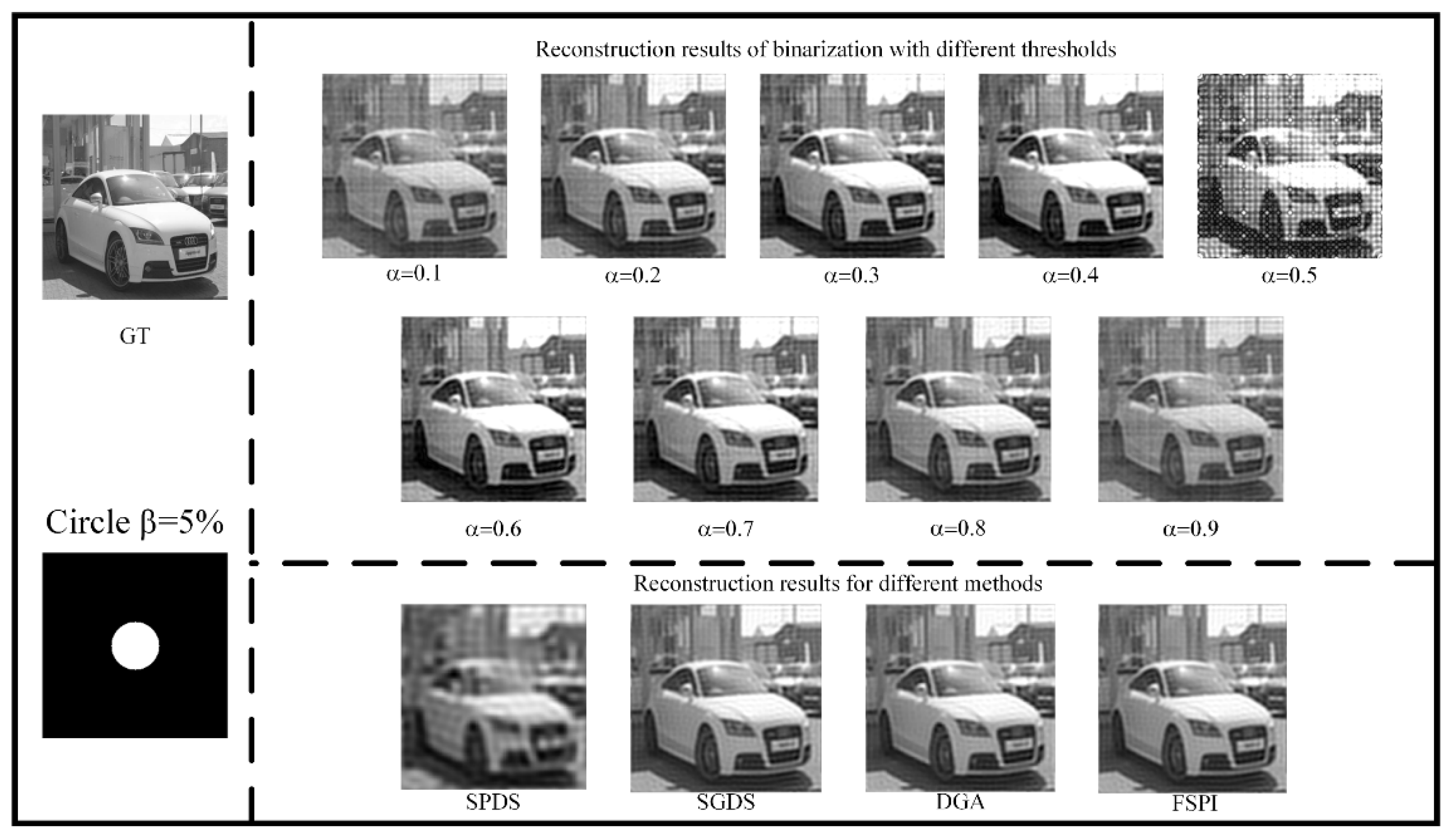
4.2. Binarization Threshold Selection Verification

In the theoretical analysis, the optimal threshold is 0.29 or 0.71. In order to prove that the threshold is binarized into the most appropriate threshold, the following simulation experiments are carried out. After normalization of the grayscale Fourier basis patterns, different thresholds were used for binarization, which were selected between 0.01 and 0.09 with an interval of 0.01, where the sampling rate is set to 5%. The circle sampling strategy was chosen as the sampling strategy. The top half of Figure 4 refers to the simulation reconstruction results of different thresholds, while the bottom half is the simulation reconstruction results of the space dithering strategy (SPDS), signal dithering strategy (SGDS), improved error diffusion jitter algorithm (DGA), and conventional Fourier single-pixel imaging (FSPI) method, respectively.

According to the upper part of Figure 4, it can be seen that at a 5% sampling rate, the quality of the pictures obtained by using different threshold simulations varies greatly. Among them, when the threshold is chosen at 0.5, the reconstructed image quality is the worst. When the threshold is small or large, the reconstructed image is visually low in brightness. When the threshold is 0.4 or 0.6, the visual effect of the image is improved compared with other thresholds. When the threshold value is 0.3 or 0.7, the visual effect is the best, and the reconstructed image is closest to the grayscale Fourier basis pattern reconstruction. The lower part of Figure 4 illustrates the reconstruction results of different binarization methods and conventional Fourier single-pixel imaging. Visually, it can be seen that SPDS has the worst reconstruction. The images reconstructed by SGDS look smoother. The simulation reconstruction result of DGA is closer to the traditional Fourier single-pixel imaging method. By comparing the other three binarization methods, it is found that when the threshold is 0.3 or 0.7, the simulation reconstruction results can achieve similar results to the conventional Fourier single-pixel imaging method.

In order to quantitatively compare the reconstruction quality with different thresholds, 1000 images were selected for the numerical simulation test. The sampling rate is fixed at 5%. The sampling strategy utilized is the circle sampling strategy. The average peak signal to noise ratio (PSNR) and structural similarity (SSIM) values of all intensity images were computed. The indices calculated for the images in the test set are shown in Figure 5.

$$PSNR=10\times {\log }_{10}\left(\frac{M^2}{\mathrm{MSE}}\right)$$

(14)

M is the maximum possible pixel value (usually 255 for an 8-bit image). MSE is the mean squared error between the original and reconstructed images, calculated as the average of the squared pixel-wise differences.

$$SSIM(x,y)=\frac{(2{\mu }_x{\mu }_y+c_1)(2{\sigma }_{xy}+c_2)}{({\mu }_x^2+{\mu }_y^2+c_1)({\sigma }_x^2+{\sigma }_y^2+c_2)}$$

(15)

x and y are the original and reconstructed images, respectively. and y are the mean pixel values of x and y. σ_x² and σ_y² are the variances of x and y. σ_xy is the covariance between x and y. c₁ and c₂ are constants to prevent instability when the denominator is close to zero.

Figure 5 shows that when the threshold is chosen from 0.01 to 0.09, the average SSNR and SSIM of the image are approximately M-shaped, and both are symmetric about 0.5. It can be seen from the figure that the threshold of 0.29 or 0.71 is the best for both PSNR and SSIM metrics. In summary, it can be concluded that the optimal threshold is 0.29 or 0.71 after theoretical and simulation analysis. Considering the real experimental situation, if the threshold is 0.71, the grayscale Fourier base pattern is greater than the threshold and set to 1, and less than the value is set to 0 to obtain the binarization Fourier basis pattern. Compared with the threshold value of 0.29, when the threshold value is 0.71, the number 1 is small, the light intensity value is small, and the ability to suppress background light is weak. Therefore, 0.29 is selected as the threshold value.

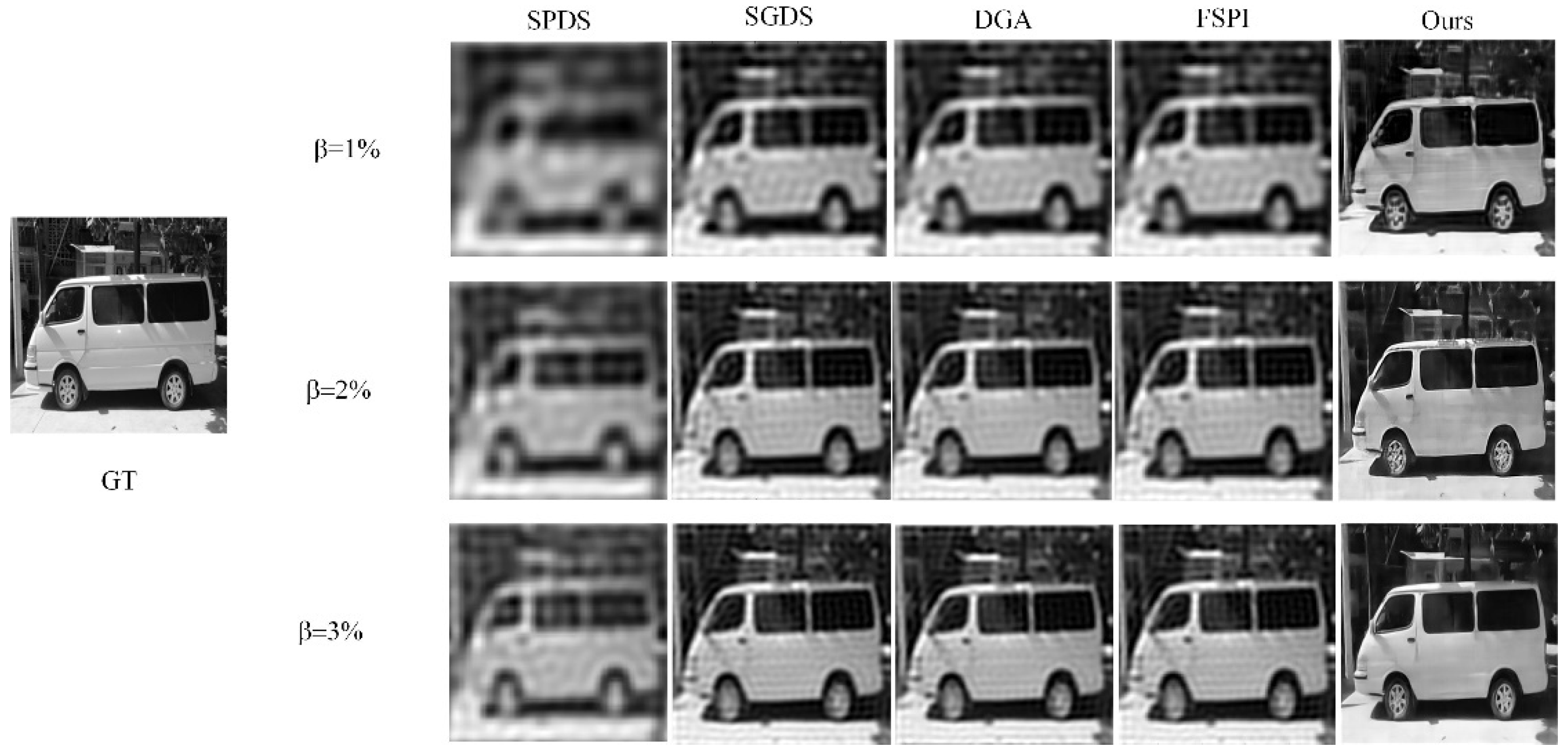
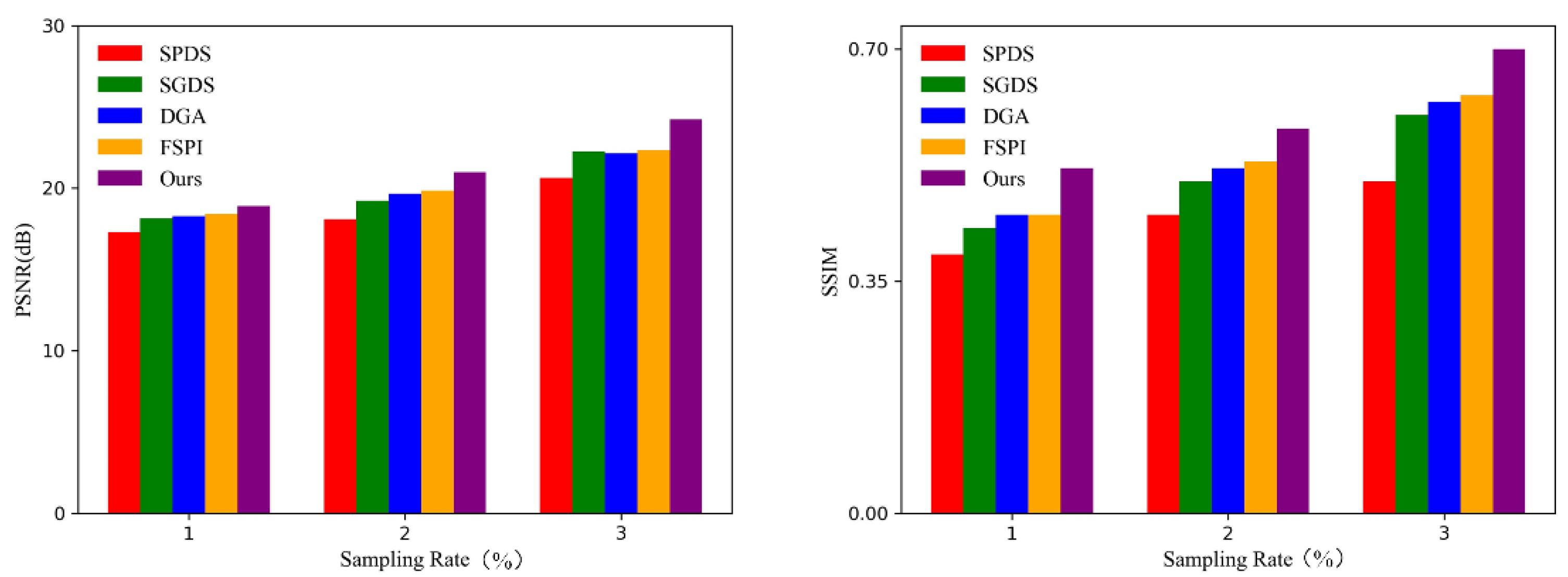
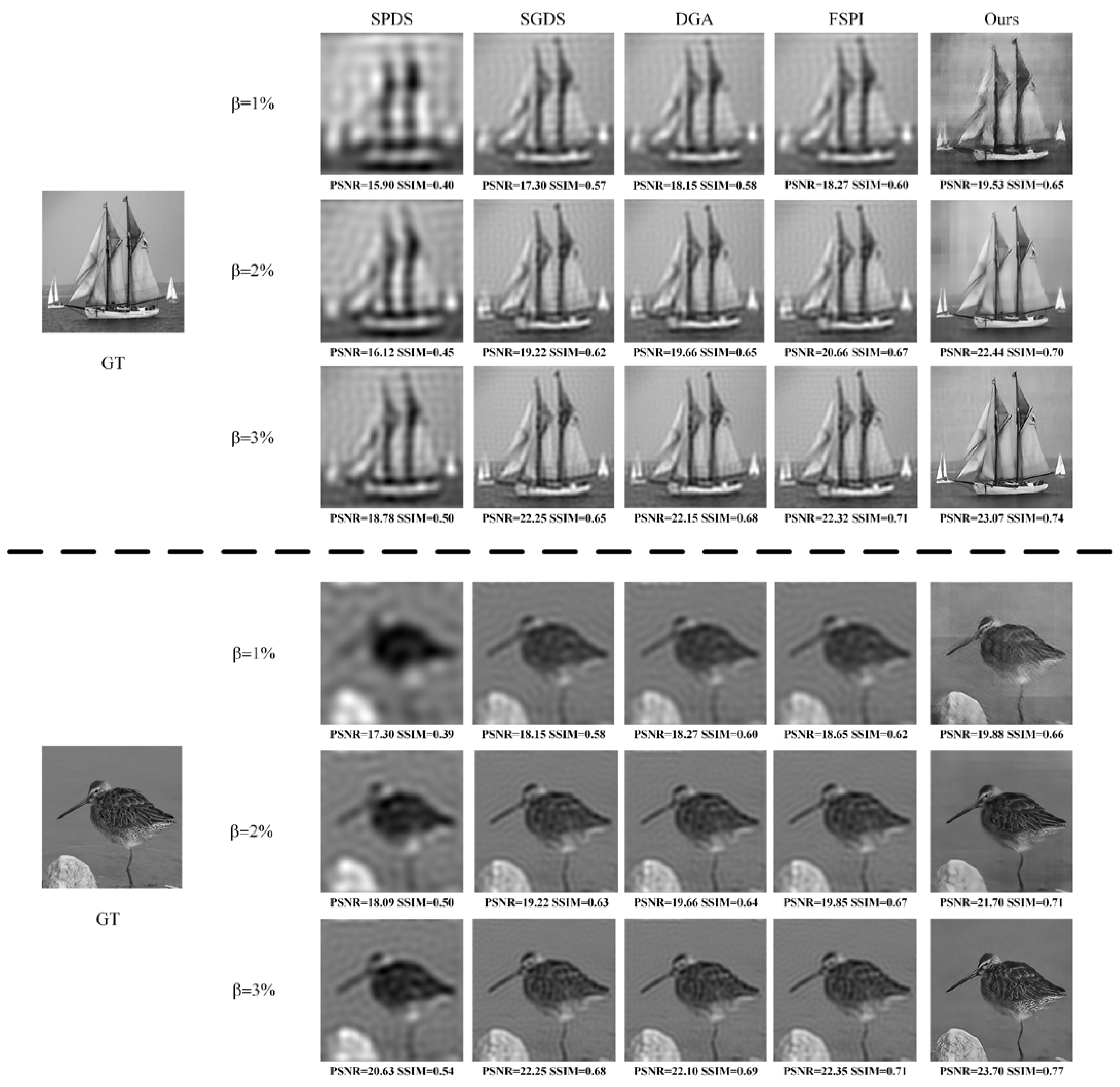
4.3. Numerical Simulations of F2SPI-GAN

The paper uses the same dataset to train images with different sample rates. Three different network models are trained for the numerical simulation, and each model corresponds to a different sampling rate of 1%, 2%, and 3%, respectively. A circle sampling strategy was used in the sampling process. The car dataset was used to train all three network models, which all share the same network architecture. Figure 6 shows the image reconstruction results with different methods and different sampling rates. The numerical simulation reconstruction results for SPDS are shown in the first column. The SGDS numerical simulation reconstruction results are shown in the second column. The DGA numerical simulation reconstruction results are shown in the third column. The fourth column shows the numerical simulation reconstruction results of the conventional FSPI method, while the fifth row demonstrates the reconstruction results obtained using the F2SPI-GAN network proposed in the paper.

From Figure 6, it is evident that the sampling rate significantly affects the quality of vehicle reconstruction. The SPDS reconstruction results are consistently the worst at any sampling rate, particularly at a sampling rate of 1%, where the overall outline of the car is barely discernible. For SGDS and DGA, although the reconstruction quality has improved, there are still noticeable blurring and ringing effects. While the image quality reconstructed by FSPI improves slightly with increasing sampling rates, these results still lack substantial, detailed information. In comparison, the proposed method exhibits superior image reconstruction clarity at any sampling rate, with minimal observable ringing artifacts. The visual results obtained using this method surpass those of other FSPI methods significantly.

In order to quantitatively evaluate the reconstruction performance of the proposed method and other methods, a test experiment was carried out. A total of 3000 images that did not appear during training make up the test set. The average PSNRs and SSIMs of the results of each method’s reconstruction are shown in Figure 7. It is shown in the figure that the SPDS method is represented in red. The SGDS method is shown in green. The DGA method is shown in blue. The orange is the conventional FSPI method. The proposed method in the paper is represented by the purple color. The sampling rate shows up in the figure’s horizontal coordinates. It is clear that when the sample rate rose, the performance metrics of all approaches got better. It is noteworthy that the approach proposed in the paper obtains the best results when compared to other methods at the same sample rate, as shown by the PSNR and SSIM indices.

To further validate the network model’s generalization ability beyond the car dataset, the paper includes testing with a sailboat image and a bird image from other natural scenes. As can be seen from Figure 8, the images reconstructed by SPDS are the worst visually and in terms of indicators. SPDS, DGA, and conventional FSPI improve the image quality visually and in terms of indicators, but there is still an obvious ringing effect. After evaluating the proposed method at different sampling rates, it is clear that the method successfully addresses the ringing artifacts that occur at low-sampling rates. Additionally, it surpasses other methods in terms of evaluation metrics. The findings highlight the efficacy of applying the network model trained on the automobile dataset to reconstructing other images. Therefore, the proposed method demonstrates strong generalization ability and can be readily employed in various real-world applications.

4.4. Real-World Experiments

The real experiment is shown in Figure 1. The laser used in the experiment is the OEM-I-532, The OEM-532-1 is manufactured by Changchun NEW INDUSTRY PHOTOelectric Technology Co. LTD. Their headquarters is located in Changchun, China. The beam diameter at the position where the laser is emitted is 10 mm. The wavelength of the laser is in the range of 531 and 533 nm. The laser was extended by a beam expander (BE02–05-A). The BE02–05-A is manufactured by Thorlabs Inc. Their headquarters is located in Newton, New Jersey, in the United States. The extended light shines in the modulation region of the DMD (V-7001). The DMD has a maximum refresh rate of 22,000 Hz, a reflectivity of 88%, and a resolution of 1024 × 768. The threshold binarization method is used to binarize the Fourier basis patterns, and the size of the Fourier base pattern is 256 × 256. The DMD is utilized to modulate the laser distribution by employing a pre-generated binarized Fourier base pattern. The optical antenna collects the light reflected from the target, which is then detected by the H11706P-01 detector. The H11706P-01 detector is manufactured by HAMAMATSU Photonics. Their headquarters is located in Hamamatsu, Japan. The detector is linked to a data acquisition card (M4X.440-X4) that records the overall light intensity. The data acquisition card has two channels with a sampling rate of 500 MS/s. The resolution of the data acquisition card is 14 or 16 bits. The target spatial spectrum is acquired using the four-step phase shift method based on the experiment. The under-sampled reconstruction result is achieved after the IFT operation. The final reconstructed image is obtained by feeding the findings of the reconstruction into the pre-trained network model.

A ‘bear’ doll model is chosen as the target scene to demonstrate the effectiveness of the proposed. The experimental scenario was performed under dark conditions. The experiment compares the proposed method to different methods. The results of the experiment align with the results of the numerical simulation, as seen in Figure 9. It can be observed that when the sampling rate advances, the quality of each method of reconstruction also increases. The reconstruction results of SPDS at different sampling rates are obviously blurred. The reconstruction results of SGDS and DGA, as well as the conventional FSPI, come with obvious ringing effects. The FSPI reconstruction’s image quality is enhanced by the F2SPI-GAN method, which can also get rid of the ringing effect. The refresh rate of the DMD is set to 2000 Hz so that the imaging quality and the imaging efficiency are combined.

In addition, in order to verify the fast Fourier single-pixel imaging method under low-sampling rates, the experimental imaging time with a sampling rate of 2% was quantitatively calculated. The sampling strategy used is a circle sampling strategy. The test platforms are Intel(R) Xeon(R) Gold 6330 CPU and RTX3090, as shown in

Table 1. Experimental imaging time.

Method	IDAQ	IIFT	IRES	IT
SPDS	1.311 s	4 ms	/	1.314 s
SGDS	7.864 s	4 ms	/	7.868 s
DGA	2.621 s	4 ms	/	2.625 s
FSPI	9.039 s	4 ms	/	9.043 s
Ours	1.311 s	4 ms	14 ms	1.329 s

. The first column represents different methods, the second column I_DAQ represents data collection time, the third column I_IFT represents inverse Fourier transform time, the fourth column I_RES represents algorithm reconstruction time, and the fifth column I_T represents the total system imaging time. The table shows that the reconstruction time of the method proposed in the paper is significantly shorter than that of SGDS, DGA, and conventional FSPI. Although the reconstruction time is the same as SPDS, the image quality is much better.

5. Discussion

This study focuses on enhancing the imaging efficiency of Fourier single-pixel imaging, thereby reducing the data acquisition time and enabling rapid reconstruction of the target scene with high-quality results. In the method, the grayscale Fourier basis pattern is binarized with a fixed threshold and modulated online into a binarized Fourier basis pattern. The reconstruction quality can be further improved by reconstructing the network at a low-sampling rate.

The experimental results show that the binarization Fourier single-pixel imaging method proposed in the paper can effectively improve image quality. The reconstructed image has higher fidelity than the original scene. Irradiation with binarized Fourier base patterns allows for faster data acquisition. In order to further improve the image quality, the under-sampled image is reconstructed through the F2SPI-GAN network. This makes it an alternative to conventional Fourier imaging methods. Binarization of Fourier single-pixel imaging has important potential in many applications. Such as 3D imaging, underwater imaging, and other areas.

In conclusion, the utilization of binarization Fourier single-pixel imaging can significantly enhance the practical implementation of Fourier single-pixel imaging. It will promote the development of Fourier single-pixel imaging.

6. Conclusions

In summary, this study proposes fast Fourier single-pixel imaging, which yields high-quality reconstruction results quickly at low-sampling rates. The method uses the idea of binarization and aims to make the DMD quickly load the binarized Fourier basis pattern. In the F2SPI-GAN model, the generator adopts an encoder-decoder structure and adds an attention block. This can enhance the quality of the reconstructed image and effectively reduce the ringing effects. The car dataset was selected to train the network model, and the trained model can quickly achieve high-quality reconstruction at a low-sampling rate. In numerical simulations and experiments, the results of the traditional FSPI are compared. The F2SPI-GAN model can shorten imaging times, remove ringing in the event of under-sampling, and enhance imaging quality. In numerical simulations and experiments, other target image types are chosen to evaluate the network model’s generalizability. The results demonstrate that the model may be used to reconstruct other natural images after being trained on the car image dataset. The method has strong generalizability and can quickly generate high-quality reconstruction results at low-sampling rates, which provides a method for fast Fourier single-pixel imaging.

References

1. Edgar, M.P.; Gibson, G.M.; Padgett, M.J. Principles and Prospects for Single-Pixel Imaging. Nat. Photonics 2019, 13, 13–20. [Google Scholar] [CrossRef]
2. Gibson, G.M.; Johnson, S.D.; Padgett, M.J. Single-Pixel Imaging 12 Years on: A Review. Opt. Express 2020, 28, 28190–28208. [Google Scholar] [CrossRef] [PubMed]
3. Li, W.; Hu, X.; Wu, J.; Fan, K.; Chen, B.; Zhang, C.; Hu, W.; Cao, X.; Jin, B.; Lu, Y.; et al. Dual-Color Terahertz Spatial Light Modulator for Single-Pixel Imaging. Light Sci. Appl. 2022, 11, 191. [Google Scholar] [CrossRef] [PubMed]
4. Olivieri, L.; Gongora, J.S.T.; Peters, L.; Cecconi, V.; Cutrona, A.; Tunesi, J.; Tucker, R.; Pasquazi, A.; Peccianti, M. Hyperspectral Terahertz Microscopy via Nonlinear Ghost-Imaging. Optica 2020, 7, 186–191. [Google Scholar] [CrossRef]
5. Ma, Y.; Yin, Y.; Jiang, S.; Li, X.; Huang, F.; Sun, B. Single Pixel 3D Imaging with Phase-Shifting Fringe Projection. Opt. Laser. Eng. 2021, 140, 106532. [Google Scholar] [CrossRef]
6. Jiang, H.; Li, Y.; Zhao, H.; Li, X.; Xu, Y. Parallel Single-Pixel Imaging: A General Method for Direct–Global Separation and 3D Shape Reconstruction Under Strong Global Illumination. Int. J. Comput. Vision 2021, 129, 1060–1086. [Google Scholar] [CrossRef]
7. Rousset, F.; Ducros, N.; Peyrin, F.; Valentini, G.; D’Andrea, C.; Farina, A. Time-resolved multispectral imaging based on an adaptive single-pixel camera. Opt. Express. 2018, 26, 10550–10558. [Google Scholar] [CrossRef]
8. Tao, C.; Zhu, H.; Wang, X.; Zheng, S.; Xie, Q.; Wang, C.; Wu, R.; Zheng, Z. Compressive Single-Pixel Hyperspectral Imaging Using RGB Sensors. Opt. Express 2021, 29, 11207–11220. [Google Scholar] [CrossRef]
9. Wu, J.; Li, S. Optical Multiple-Image Compression-Encryption via Single-Pixel Radon Transform. Appl. Opt. 2020, 59, 9744–9754. [Google Scholar] [CrossRef]
10. Deng, Q.; Zhang, Z.; Zhong, J. Image-free real-time 3-D tracking of a fast-moving object using dual-pixel detection. Opt. Lett. 2020, 45, 4734–4737. [Google Scholar] [CrossRef]
11. Zha, L.; Shi, D.; Huang, J.; Yuan, K.; Meng, W.; Yang, W.; Jiang, R.; Chen, Y.; Wang, Y. Single-Pixel Tracking of Fast-Moving Object Using Geometric Moment Detection. Opt. Express 2021, 29, 30327–30336. [Google Scholar] [CrossRef]
12. Wu, J.; Hu, L.; Wang, J. Fast Tracking and Imaging of Moving Object with Single-Pixel Imaging. Opt. Express 2021, 29, 42589–42598. [Google Scholar] [CrossRef]
13. Deng, S.; Liu, W.; Shen, H. Laser Polarization Imaging Method Based on Frequency-Shifted Optical Feedback. Opt. Laser. Technol. 2023, 161, 109099. [Google Scholar] [CrossRef]
14. Yu, T.; Wang, X.; Xi, S.; Mu, Q.; Zhu, Z. Underwater Polarization Imaging for Visibility Enhancement of Moving Targets in Turbid Environments. Opt. Express 2023, 31, 459–468. [Google Scholar] [CrossRef] [PubMed]
15. Yang, X.; Yu, Z.; Xu, L.; Hu, J.; Wu, L.; Yang, C.; Zhang, W.; Zhang, J.; Zhang, Y. Underwater Ghost Imaging Based on Generative Adversarial Networks with High Imaging Quality. Opt. Express 2021, 29, 28388–28405. [Google Scholar] [CrossRef] [PubMed]
16. Yang, X.; Yu, Z.; Jiang, P.; Xu, L.; Hu, J.; Wu, L.; Zou, B.; Zhang, Y.; Zhang, J. Deblurring Ghost Imaging Reconstruction Based on Underwater Dataset Generated by Few-Shot Learning. Sensors 2022, 22, 6161. [Google Scholar] [CrossRef]
17. Wang, F.; Wang, C.; Chen, M.; Gong, W.; Zhang, Y.; Han, S.; Situ, G. Far-Field Super-Resolution Ghost Imaging with a Deep Neural Network Constraint. Light Sci. Appl. 2022, 11, 1. [Google Scholar] [CrossRef]
18. Ma, S.; Liu, Z.; Wang, C.; Hu, C.; Li, E.; Gong, W.; Tong, Z.; Wu, J.; Shen, X.; Han, S. Ghost Imaging LiDAR via Sparsity Constraints Using Push-Broom Scanning. Opt. Express 2019, 27, 13219–13228. [Google Scholar] [CrossRef] [PubMed]
19. Li, R.; Hong, J.; Zhou, X.; Li, Q.; Zhang, X. Fractional Fourier Single-Pixel Imaging. Opt. Express 2021, 29, 27309–27321. [Google Scholar] [CrossRef]
20. Gao, Z.; Li, M.; Zheng, P.; Xiong, J.; Tang, Z.; Liu, H. Single-pixel imaging with Gao-Boole patterns. Opt. Express 2022, 30, 35923–35936. [Google Scholar] [CrossRef]
21. He, R.; Weng, Z.; Zhang, Y.; Qin, C.; Zhang, J.; Chen, Q.; Zhang, W. Adaptive Fourier Single Pixel Imaging Based on the Radial Correlation in the Fourier Domain. Opt. Express 2021, 29, 36021–36037. [Google Scholar] [CrossRef] [PubMed]
22. Zhao, Y.-N.; Hou, H.-Y.; Han, J.-C.; Cao, D.-Z.; Zhang, S.-H.; Liu, H.-C.; Liang, B.-L. Complex-Amplitude Fourier Single-Pixel Imaging via Coherent Structured Illumination. Chin. Phys. B 2022, 32, 064201. [Google Scholar] [CrossRef]
23. Wenwen, M.; Dongfeng, S.; Jian, H.; Kee, Y.; Yingjian, W.; Chengyu, F. Sparse Fourier Single-Pixel Imaging. Opt. Express 2019, 27, 31490–31503. [Google Scholar] [CrossRef] [PubMed]
24. Qiu, Z.; Guo, X.; Lu, T.; Qi, P.; Zhang, Z.; Zhong, J. Efficient Fourier Single-Pixel Imaging with Gaussian Random Sampling. Photonics 2021, 8, 319. [Google Scholar] [CrossRef]
25. Rizvi, S.; Cao, J.; Zhang, K.; Hao, Q. Improving Imaging Quality of Real-Time Fourier Single-Pixel Imaging via Deep Learning. Sensors 2019, 19, 4190. [Google Scholar] [CrossRef]
26. Zhang, Z.; Wang, X.; Zheng, G.; Zhong, J. Fast Fourier Single-Pixel Imaging via Binary Illumination. Sci. Rep. 2017, 7, 12029. [Google Scholar] [CrossRef]
27. Huang, J.; Shi, D.; Yuan, K.; Hu, S.; Wang, Y. Computational-Weighted Fourier Single-Pixel Imaging via Binary Illumination. Opt. Express 2018, 26, 16547–16559. [Google Scholar] [CrossRef]
28. Li, J.; Cheng, K.; Qi, S.; Zhang, Z.; Zheng, G.; Zhong, J. Full-resolution, full-field-of-view, and high-quality fast Fourier single-pixel imaging. Opt. Lett. 2023, 48, 49–52. [Google Scholar] [CrossRef]
29. Yang, X.; Jiang, P.; Jiang, M.; Xu, L.; Wu, L.; Yang, C.; Zhang, W.; Zhang, J.; Zhang, Y. High Imaging Quality of Fourier Single Pixel Imaging Based on Generative Adversarial Networks at Low Sampling Rate. Opt. Lasers Eng. 2021, 140, 106533. [Google Scholar] [CrossRef]
30. Jiang, P.; Liu, J.; Wu, L.; Xu, L.; Hu, J.; Zhang, J.; Zhang, Y.; Yang, X. Fourier Single Pixel Imaging Reconstruction Method Based on the U-Net and Attention Mechanism at a Low Sampling Rate. Opt. Express 2022, 30, 18638–18654. [Google Scholar] [CrossRef]
31. Falk, T.; Mai, D.; Bensch, R.; Çiçek, Ö.; Abdulkadir, A.; Marrakchi, Y.; Böhm, A.; Deubner, J.; Jäckel, Z.; Seiwald, K.; et al. U-Net: Deep Learning for Cell Counting, Detection, and Morphometry. Nat. Methods 2019, 16, 67–70. [Google Scholar] [CrossRef] [PubMed]
32. Schlemper, J.; Oktay, O.; Schaap, M.; Heinrich, M.; Kainz, B.; Glocker, B.; Rueckert, D. Attention Gated Networks: Learning to Leverage Salient Regions in Medical Images. Med. Image Anal. 2019, 53, 197–207. [Google Scholar] [CrossRef] [PubMed]
33. Mao, X.-J.; Shen, C.; Yang, Y.-B. Image Restoration Using Very Deep Convolutional Encoder-Decoder Networks with Symmetric Skip Connections. Advances in Neural Information Processing Systems 29. 2016. Available online: https://proceedings.neurips.cc/paper_files/paper/2016/hash/0ed9422357395a0d4879191c66f4faa2-Abstract.html (accessed on 21 August 2016).
34. Rajinikanth, V.; Joseph Raj, A.N.; Thanaraj, K.P.; Naik, G.R. A Customized VGG19 Network with Concatenation of Deep and Handcrafted Features for Brain Tumor Detection. Appl. Sci. 2020, 10, 3429. [Google Scholar] [CrossRef]
35. Krause, J.; Stark, M.; Deng, J.; Fei-Fei, L. 3D Object Representations for Fine-Grained Categorization. In Proceedings of the IEEE International Conference on Computer Vision Workshops, Sydney, NSW, Australia, 2–8 December 2013; pp. 554–561. [Google Scholar] [CrossRef]
Figure 1. Schematic diagram of the Fourier single-pixel imaging system.
Photonics 10 00963 g001
Figure 2. The overall network structure of F2SPI-GAN. (a) Architecture of F2SPI-GAN generator; (b) Architecture of F2SPI-GAN discriminator; (c) Attention-block structure.
Photonics 10 00963 g002
Figure 3. (ac) Training loss at different sampling rates.
Photonics 10 00963 g003
Figure 4. Reconstruction results for different Fourier basis patterns at a 5% sampling rate.
Photonics 10 00963 g004
Figure 5. The average PSNR and SSIM under different thresholds.
Photonics 10 00963 g005
Figure 6. Car results for the reconstruction of different methods.
Photonics 10 00963 g006
Figure 7. Average PSNR and SSIM of images reconstructed by different methods.
Photonics 10 00963 g007
Figure 8. Sailboat and bird images reconstructed by FSPI and the proposed method.
Photonics 10 00963 g008
Figure 9. Different methods to reconstruct the experimental results of “Bear”.
Photonics 10 00963 g009