1. Introduction
External cavity feedback is a common scheme for laser linewidth narrowing. At present, a lot of work has been conducted to narrow the linewidth through the external cavity. The external cavity scheme is mainly based on Littrow or Littman structures [
1,
2]. Considering the volume of blazed grating and other issues, more Littrow-like or Littman-like structures based on non-blazed grating forms appear. The core of each scheme involves screening and locking the optical frequency in the external cavity, and then suppressing the edge mode noise to narrow the laser linewidth. In addition to the blazed grating, many excellent works have successively developed other devices to meet the requirements of the scheme, including Bragg volume grating [
3,
4,
5], Fabry–Pérot etalon (FP) [
6], fiber grating [
7,
8], planar lightwave circuit (PLC) [
9,
10,
11], quantum dot lasers [
12,
13], etc. Many of them have been applied to engineering practices.
After the continuous advancement of applications, especially after the integration of lasers, the external cavity feedback semiconductor laser has obvious bistability, including optical longitudinal mode bistability [
14,
15,
16,
17] and optical transverse mode (polarization) bistability [
18,
19]. This phenomenon causes laser mode hopping during disturbances, which can affect the stability of the laser output. In addition to bistability, lasers also exhibit other dynamic characteristics, such as stable fixed points [
20,
21], quasi-periodic [
22,
23], chaos [
24,
25], etc. These characteristics will also affect the mode hopping behavior of the laser. The research on mode hopping of external cavity semiconductor lasers is mainly divided into two aspects: experimental measurement and theoretical analysis. The experimental measurement [
26,
27] is mainly focused on finding novel and reliable measurement methods of mode hopping. The main ideas of theoretical analysis [
28,
29] are focused on discussing and analyzing the output advantages of several competitive models. However, in the literature, there has been no discussion of directly correlating bistability with the thermal synchronization problem.
In this work, we chose a general configuration to build our integrated external cavity narrow linewidth semiconductor laser. Based on the laser, we found that the experimental results have optical bistability and time inversion asymmetry. This result is also consistent with the measurement results of commercial devices of similar schemes. It has strong reproducibility. In order to understand this phenomenon, we first simulated the model results with perfect time-inversion symmetry as a reference. Then we found and explained the origin of this thermal tuning asymmetry based on the device characteristics. Finally, by taking into account the factors we discovered in our model, we explain this phenomenon.
2. Configuration and Methods
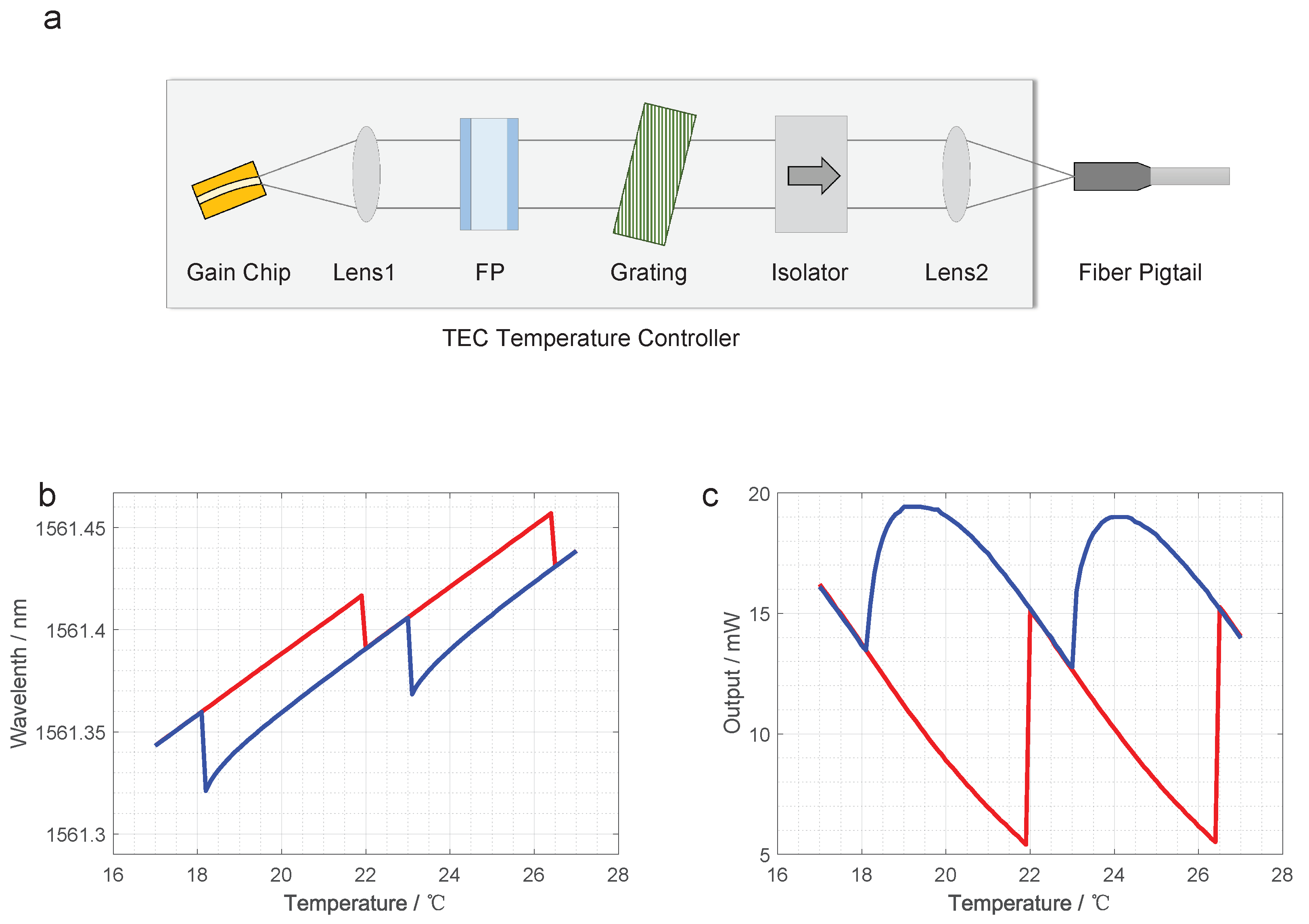
The schematic diagram of a typical external cavity feedback semiconductor laser (ECL) is shown in
Figure 1a. The laser consists of a gain chip, a Fabry–Pérot etalon (FP), a volume Bragg grating, an isolator, two lenses, and a thermoelectric cooling (TEC) temperature controller. The gain chip provides gain for laser oscillation. One end of the gain chip has high reflectivity and the other end has high transmissivity. The high-reflectivity end acts as the mirror of the external cavity to reflect light, and the other end with high transmissivity faces the interior of the cavity to facilitate the entrance and exit of the resonant light. FP can purify resonance light and select longitudinal mode. The bandwidth of the FP is 7.5 GHz in this paper. The filter bandwidth of volume Bragg grating is 125 GHz, which acts as the cavity mirror at the output side of the external cavity and can purify the longitudinal mode of the output light. The isolator ensures the isolation of the external cavity of the laser from the outside. Lens 1 plays the role of beam expansion, so that the small aperture beam inside the gain chip can be coupled with the external cavity, and lens 2 shapes the output beam and couples it with the fiber tailpipe. The TEC temperature controller is used to keep the temperature of the plane constant, where the whole cavity is located, especially in the area near the gain chip. The entire external cavity is assembled on a substrate, and the TEC temperature controller controls the substrate temperature, so as to keep the temperature of the entire external cavity constant, especially the area near the gain chip.
The external cavity filter laser’s frequency is in the form of an optical comb, and its equivalent length determines the frequency of a single longitudinal mode and the interval between each longitudinal mode. The equivalent length
of the external cavity is defined as the sum of the product of the refractive index
and the length of each segment
in the cavity.
The summation section includes information about the gain chip, lens, FP, and the gas components of each component.
In the optical comb, the integral
N time of each wavelength
must be the same as the equivalent cavity length, so the equivalent cavity length can also be written as
Conversely, the longitudinal mode wavelength
corresponding to the comb near a certain wavelength
can be solved as follows:
where the operator
represents rounding.
According to Equation (
2), for a given longitudinal mode wavelength
, the wavelength interval
of the comb can be obtained by
Therefore, the function of the optical comb near
can be written as
is a variable that represents the wavelength.
is the unit pulse sequence in the discrete domain,
In practice, it is not easy to calculate the equivalent external cavity length by Equation (
1), but the frequency interval at the specified frequency can be measured. According to Equation (
4) for a given longitudinal mode wavelength
and a given wavelength interval
of the comb, the equivalent cavity length can also be written as
Through the above equations and experimental results in
Figure 1b, we can simulate the optical comb and obtain all its properties. It turns out that the optical comb redshifts with the increase in temperature.
FP filtering selects the longitudinal mode in the external cavity through its narrow filtering bandwidth. Similar to the external cavity, the central wavelength of the FP’s filtering bandwidth is related to its equivalent length
, where
is the actual length of the FP, and
is the refractive index of the FP. They are both temperature-related. Because the temperature range involved in this work is narrow, we can assume that the refractive index and actual length meet the linear relationship with temperature in this range. Therefore, they can be simply expressed as linear functions of the temperature
T.
is the linear thermal expansion coefficient of quartz, in the order of
[
30].
is the refractive index temperature coefficient of quartz, which is negative and in the order of
[
31]. The central wavelength frequency
of the FP filtering bandwidth near a given wavelength
can be calculated by
and
.
is much larger than
, the negative drift of the refractive index dominates the drift of the FP central wavelength. This results in the FP central wavelength
experiencing a blue shift as the temperature rises.
Since the filtering bandwidth of the FP is much larger than the linewidth of each longitudinal mode in the comb, the shape of the FP filtering curve also needs to be considered. In general, the passband filtering curve of the FP meets the Lorentz distribution; that is
is a variable that represents the wavelength.
represents the filtering bandwidth of the FP and is the FWHM of the Lorentz distribution. In this work,
GHz. The first numerator
on the right of the equal sign is a normalization coefficient, which guarantees that the maximum value of this curve is 1.
The grating is similar to the FP, but it has a much wider filtering bandwidth of 125 GHz, so the passband filtering function of the grating is directly given here:
is a variable that represents the wavelength.
represents the filtering bandwidth of the grating and corresponds to the FWHM of the Lorentz distribution. The center wavelength of the grating is
. The first numerator
on the right of the equal sign is a normalization coefficient, guaranteeing that the maximum value of this curve is 1.
The wavelength selectivity of the laser in this work is composed of the external cavity comb, the FP, and grating. The gain of the optical gain chip can be considered flat in a small wavelength range. So, only considering the static process, the longitudinal mode with the lowest loss can obtain a competitive advantage and output. For the laser in this work, the normalized comprehensive loss function is
When discussing the competition of modes in the early stage of resonance, the above equation derives the screening losses of different modes. In addition to this, the so-called Bogatov effect [
32] needs to be taken into account in the calculation. Due to nonlinear effects, such as four-wave mixing, adjacent short-wavelength modes provide additional gain for long-wavelength modes when multiple modes coexist. In Ref. [
33], according to the model of Lenstra et al., the Bogatov dynamic gain can be written as
is the gain coefficient of the short-wavelength mode.
and
are the linear gains for the short-wavelength and long-wave modes, respectively.
is the linewidth parameter of the short-wavelength mode.
is the lifetime of the long-wave modes.
is the angular mode-frequency difference between the short-wavelength and long-wave modes. In this work,
is taken as
GHz, and the remaining parameters will follow the original model.
is the power of the short-wavelength mode. Taking into account the Bogatov effect, the output power
rate equation corresponding to the external cavity feedback is
t is the time.
R is the spontaneous emission rate.
is the cavity loss rate.
g is the linear gain.
is the differential gain coefficient.
is the average inversion available for lasing. This work discusses the competition of modes before lasing. At this point,
R and
can be considered very small. Therefore, Equation (
15) can be simplified as
Linear gain g is provided by the gain chip. Within a smaller range, the linear gain can be considered flat. The cavity loss rate
can be calculated by Equation (
13). The time of mode establishment is very short. It is generally on the order of
[
33,
34]. For ease of processing, in this work, the mode establishment time is taken as
ns, and
is simply integrated with
. The result of the integration is used as the Bogatov gain during each mode establishment round. This method can effectively preserve the positive correlation between the gain and short wavelength mode power, as well as simplify the calculation.
Figure 1b,c show the experimental measurement data. The pump current of the laser is kept at 160 mA. The temperature is controlled by TEC, and the temperature value is measured by a thermistor attached to the optical gain chip. After each temperature adjustment, the data measurement record will wait until the laser is completely stable. The laser output optical wavelength is measured by a Yokogawa AQ6151B wavelength meter. The laser output power is measured by a Thorlabs S146C photodetector, and is read by a Thorlabs PM100D console.
3. Result and Discussion
The equivalent length of the external cavity changes with the substrate temperature changing, which leads to the drift of the longitudinal mode wavelength. Therefore, the laser wavelength can be tuned in a small range by changing the control temperature of the substrate. In this process, we observed that the direction of temperature tuning affects the output of the longitudinal mode of the laser, as shown in
Figure 1b,c.
Figure 1b shows the corresponding relationship between the laser output wavelength and temperature.
Figure 1c shows the corresponding relationship between the laser output power and temperature. In these two figures, the curves of different colors correspond to different temperature-changing directions. The blue line represents the cooling process, and the red line represents the heating process. Each data point is a steady-state result measured after reaching the thermal equilibrium. One interesting point is that, at the same temperature, the difference between the heating and cooling process will lead to different output modes, and the two longitudinal modes can maintain stable outputs. This means that the laser resonator exhibits bistability. Moreover, in the data of the heating process, the longer wavelength mode with lower output power will be more competitive and stable than the shorter wavelength mode with higher output power. In addition, it can be observed that during the cooling process, when the output power of the laser reaches its maximum, there appears to be a power saturation zone. After going through the saturation zone, the power drops rapidly and mode hopping occurs.
Using Equation (
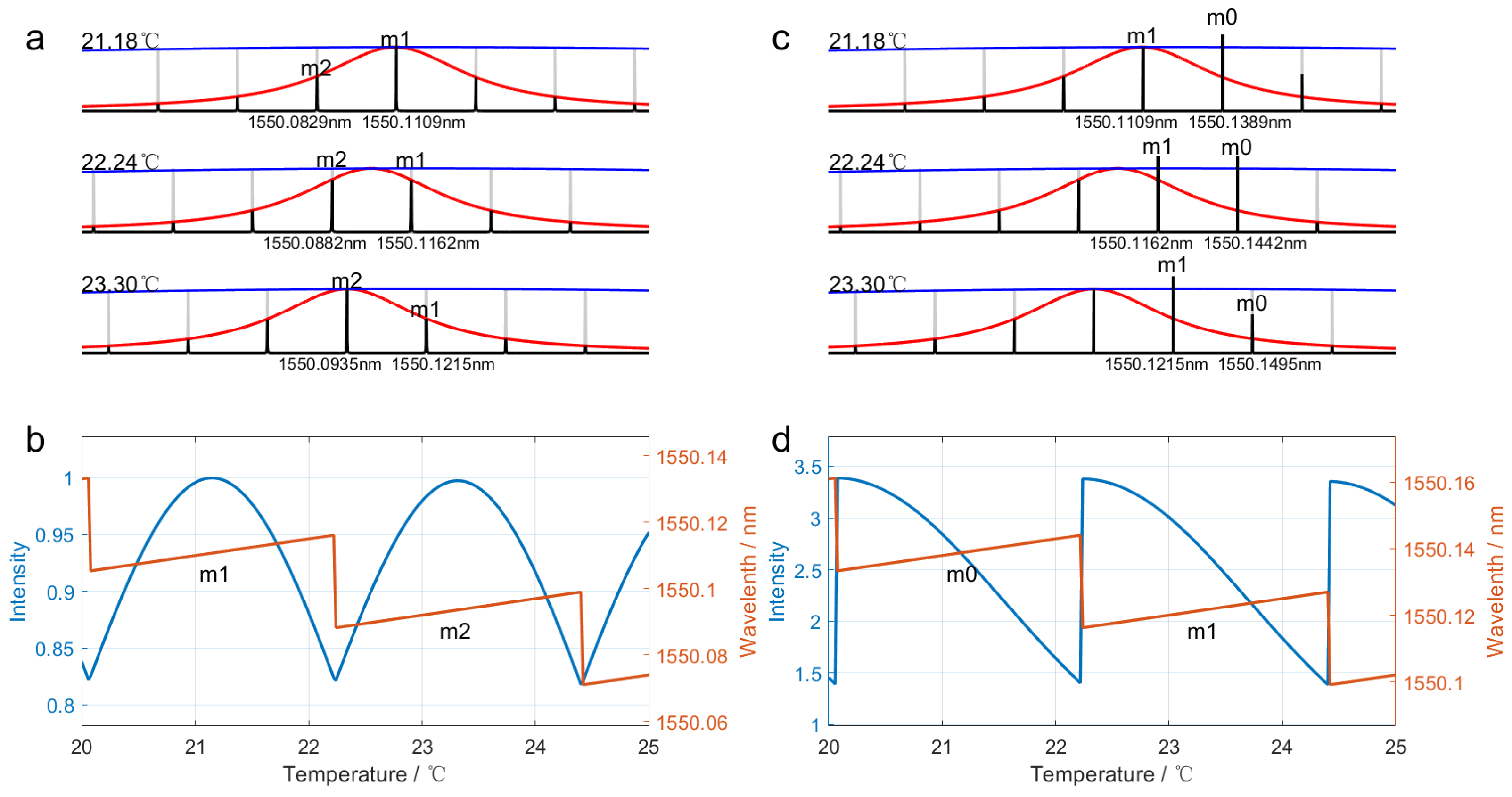
13), we can simulate the relationship between the laser output mode and temperature. For convenience, the central wavelength is set as 1550 nm, which will not affect the presentation of the simulation results. Since the relevant derivation does not contain time-related variables, the content of the analytical model is time-inversion symmetric. This means that any operation can be canceled by the reverse operation. For three typical temperatures, the distribution of each curve is shown in
Figure 2a. The comb-like light gray curve corresponds to the optical comb curve, which is obtained from the external cavity equation of Equation (
5). The Lorentz-shaped red curve corresponds to the curve of the FP, which is obtained from the FP equation of Equation (
11). The blue curve represents the grating curve obtained from the grating equation of Equation (
12). It is also a Lorentz-shaped curve, but it is close to a straight line in the figure because its FWHM is far greater than the FP curve. The comb-shaped black curve with various intensities represents the product of the previous three curves, derived from Equation (
13). As shown in
Figure 2a, at 21.18
C, the attenuation of the
mode is the lowest, giving it a competitive edge for the output. With the increase in temperature, both the FP and grating curves exhibit a blue shift, and the comb shifts red. The wavelength of the
mode becomes larger, and the attenuation also increases. When the temperature reaches 22.24
C, the attenuation of the
mode is lower than the
mode for the first time, and the
mode gains a competitive advantage. Then mode hopping occurs, and the wavelength of the
mode starts to output. With the temperature increasing, the wavelength of the
mode becomes larger, and its intensity gradually increases with attenuation decreasing. At 23.30
C, the attenuation of the
mode is the lowest, and its intensity is the largest. This process is reciprocal. The bistability will only occur when the attenuation levels of the two modes are close, as seen near 22.4 °C in
Figure 2a. This is because the above system is time-reversal symmetry. However, the characteristics revealed by the experimental data cannot be possessed by a time-reversal symmetry system. As a result, this physical model with time-inversion symmetry can only obtain the temperature tuning curve, as shown in
Figure 2b. The heating and cooling processes are consistent. This is inconsistent with the experimental data.
After considering the Bogatov effect, the long-wavelength mode gains a significant advantage in the mode competition.
Figure 2c shows this feature. The
mode in
Figure 2c does not originally have a competitive advantage due to FP filtering, but with the help of the Bogatov effect, the
mode can achieve higher intensity than the
mode and prevail in the mode competition, resulting in its output. Therefore, the Bogatov effect causes the temperature tuning curve of the laser to exhibit significant asymmetry, as shown in
Figure 2d. In
Figure 1b,c, the temperature tuning curve of the laser is always dominated by the long-wavelength mode. The introduction of the Bogatov effect explains this characteristic well. The shape of the curve in
Figure 2d is also similar to the real tuning curve. However, the tuning curve here is still insensitive to the tuning direction. Every temperature tuning is accompanied by a change in cavity length. It corresponds to the process of the original mode’s mismatch and the reestablishment of the new mode. After the dissonance of the cavity, the previously competitive mode was reshuffled. As long as the initial conditions are consistent, the output of the pattern is always consistent, independent of the path that reaches the initial conditions. That is to say, after considering the Bogatov effect, although the symmetry of the mode gain is broken, the equation is still time-reversal symmetric. In order to obtain the experimental results, there must be other mechanisms that introduce time-reversal asymmetry.
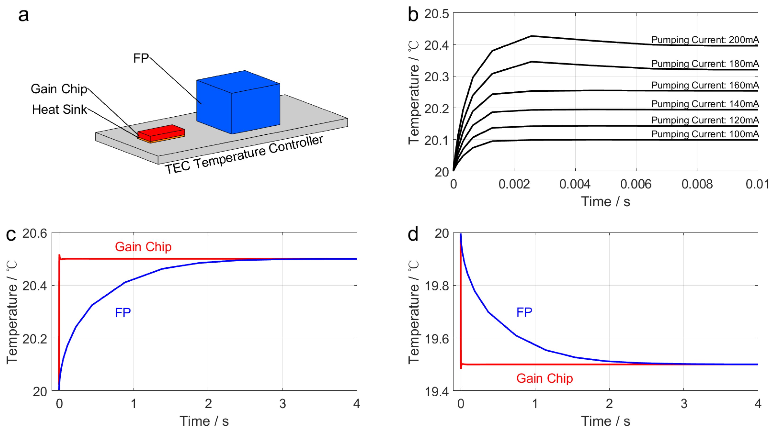
Consider the time. The above deduction implies that various operations occur at the same time. For example, it is implicitly assumed that the red-shift of the external cavity comb and the blue shift of the FP curve occur simultaneously and work together. In fact, due to the difference in the electron transition time and thermal conduction time, the operations of each part are not synchronous. In order to explain the difference, we carried out several thermal simulations of the external cavity’s structural components.
The schematic diagram of the thermal simulation structure is shown in
Figure 3a. It is assumed that the upper surface of the temperature controller always maintains a constant temperature and has good thermal contact with the lower surface of each device. The adiabatic approximation is made for the other surfaces of all devices. We carried out simulations for three different scenarios: a simulation of the chip’s active working temperature increase (
Figure 3b) as well as passive heating (
Figure 3c) and cooling (
Figure 3d) simulations. In
Figure 3b, the gain chip is considered a constant power heat source, and different pump currents represent different levels of heating power. The thermal stability time of the gain chip is in the order of
s under a conventional pump current injection. In
Figure 3c,d, the gain chip and FP are passively heated and cooled. In these processes, the thermal balance time of the gain chip is still in the order of
s, while the thermal balance time of the FP is as long as (approximately) 3 s. Due to the difference in the thermal balance time order of magnitude, the temperature change process of the gain chip is almost instantaneous compared with that of the FP. The temperature change of the gain chip plays a dominant role in the frequency drift of the external cavity comb, while the temperature change of the FP leads to the frequency drift of its passband curve. Therefore, during each temperature change process, the frequency drift of the external cavity optical comb always precedes the frequency drift of the FP passband filtering curve. The grating is similar to the FP. In addition, the average lifetime of the upper level in an excited atom is in the order of
s [
34], which is much shorter than the time required for thermal equilibrium. Therefore, for each temperature change process, the laser’s interior will experience three processes with obvious sequences. That is, after the longitudinal mode is established, the optical comb is just starting its shift. After the optical comb completes its shift, the FP and grating curves still slowly continue their movement processes. The time sequences of these three processes are fixed, independent of the heating and cooling directions. This means that heating and cooling are not mutually inverse processes. These strict three-step sequences break the time-inversion symmetry.
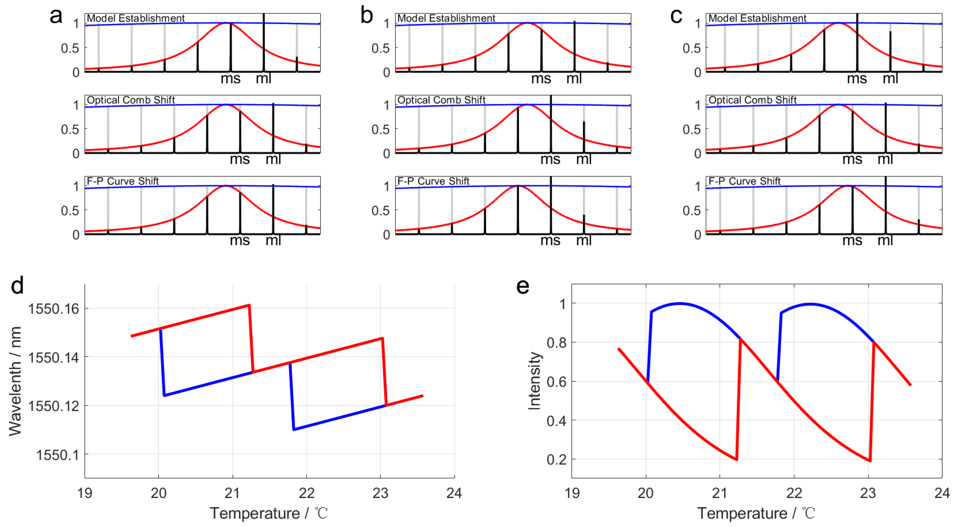
For convenience, in this work, these three-step sequences will be called mode establishment, optical comb shift, and the FP curve shift, respectively.
Figure 4a–c show three typical processes, including this three-step sequence.
Figure 4a shows the output process of the longitudinal mode following power activation. During the mode establishment process, thanks to the Bogatov effect, the long-wavelength mode
obtained higher gain than the short-wavelength mode
, which had an advantage in the competition and resonant output. During the optical comb shift process, undergoes a red-shift, and the cycle of mode misalignment and reestablishment persists. Although the transmissivity of the long-wavelength mode
is lower than that of the short-wavelength
mode, thanks to the Bogatov effect, the long-wavelength mode retains its competitive edge and achieves output. During the FP curve shift process, since the temperature of the FP has not changed, the state of this process is consistent with the previous process. This is similar to the process with the Bogatov effect considered in
Figure 2c. This indicates that with the long-wavelength mode
, it is always easier to obtain resonant output than in the short-wavelength mode
.
Figure 4b shows the mode hopping process of the laser when the temperature rises. During the mode establishment process, with the help of the Bogatov effect, the laser maintains the initial state of the long-wavelength mode
output, even under low transmittance conditions. During the optical comb shift process, the optical comb red-shifts; the transmission of the long-wavelength mode
becomes low enough and is unable to maintain a competitive advantage. Therefore, the short-wavelength mode
, which simultaneously has very high transmittance and the Bogatov gain, retains its competitive edge and resonant output; moreover, laser mode hopping occurs. During the FP curve shift process, the FP curve blue-shifts. It further guarantees the side-mode suppression ratio suppression ratio of the short-wavelength mode
. There is one more thing that needs to be explained here. The optical comb shift process is accompanied by mode misalignment and subsequent realignment, which is a prerequisite for the occurrence of mode hopping. However, during this process, the filtering conditions of the FP have not changed. The laser operates in a state where mode hopping is less likely to occur. Therefore, lasers require higher tuning temperatures for mode hopping to occur. Here, the tuning direction has an impact on the tuning results.
Figure 4c shows the mode hopping process of the laser when the temperature reduces. During the mode establishment process, the laser maintains the initial state of the short-wavelength mode
output. During the optical comb shift process, the optical comb blue-shifts, the transmission of the short-wavelength mode
reduces, and the transmission of the long-wavelength mode
increases. Different from the temperature rise mode hopping process, the dominant mode
is in the gain saturation state at this time, which cannot effectively inhibit the gain rise of other modes. Therefore, due to its high transmittance and higher Bogatov gain, the long-wavelength mode
is able to dominate the mode competition and output. Laser mode hopping occurs. During the FP curve shift process, the FP curve red-shifts. It further reduces the transmissivity of the short-wavelength mode
and helps the long-wavelength mode
obtain advantages. This shows that the short-wavelength mode struggles to maintain its competitive advantage under the condition of gain saturation.
Through the above analysis, we can see that there are significant differences between the heating and cooling processes of the lasers. The Bogatov effect gives long-wavelength modes an advantage in mode competition. This results in an asymmetric shape in the temperature tuning curve. The three-step sequences allow the tuning directions to affect the tuning results, causing inconsistencies in the heating and cooling tuning curves of our laser. Based on this model, we recalculate the curves of the laser wavelength tuning and tuning power, respectively. The mode intensity is still calculated using the filtering curve and Bogatov effect, and the mode with the highest intensity is taken as the output mode. The results are shown in
Figure 4d,e. It can be seen that the simulation results clearly capture the features of the experimental observation shown in
Figure 1b,c. There are slight differences in wavelength values between the simulation and experimental data. This is because there is a slight deviation between the actual refractive index in each medium and the simulated ones. There are also slight differences between the simulation and experimental data of the laser output intensity, as the model does not take into account factors such as laser coupling efficiency. However, even without considering these factors, the trends in the simulation results are consistent with the experimental data. This model is a good indication of the physical nature of laser tuning characteristics. The characteristics of optical components and thermal asynchrony together lead to the experimental results in
Figure 1b,c. This ultimately causes the tuning characteristics of the laser to exhibit significant bistability and tuning direction dependence.


