Focusing of Radially Polarized Electromagnetic Waves by a Parabolic Mirror

Abstract

It is well-known that a strong longitudinal electric field and a small spot size are observed when radially polarized beams are tightly focused using a high numerical aperture parabolic mirror. The longitudinal electric field component can accelerate electrons along the propagation axis at high intensities in the focal region, which opens an application in particle acceleration. In this paper, we present a rigorous derivation of the electric field obtained when a radially polarized, monochromatic, flat-top beam is focused by a parabolic mirror. The formulae were deduced from the Stratton–Chu integral known from vector diffraction theory. We examined the influence of the focusing parameters on the distribution of both the longitudinal and radial electric field components. In the small numerical aperture and short wavelength regimes, excellent agreement was found with the results obtained from the Rayleigh–Sommerfeld formula. The calculation method can be adapted for various beam types and for electromagnetic pulses as well.

1. Introduction

The paraboloid mirror can focus light nearly within a 4π solid angle [1,2]. Because of this special characteristic, researchers have been strongly interested in parabolic mirrors over the past several decades. The vector field nature of the light becomes essential in accurate description of a nonparaxial beam, when a beam is tightly focused by a parabolic mirror. The high-intensity laser community, which makes major efforts to achieve the highest laser intensities, is strongly interested in examinations of the vector field focusing characteristics [3]. By tightly focusing the beam in a vacuum using an off-axis parabolic (OAP) mirror, it is possible to attain extremely high intensity, which makes this of interest for laser-based particle acceleration [4]. For such a high-intensity, tightly focused electromagnetic field, a detailed description of the focused field is necessary in order to precisely identify the motion of charged particles [5]. Using a high numerical aperture parabolic mirror with a radially polarized beam is ideal for achieving a small focal spot size and strong longitudinal electric field, which opens an application possibility in particle acceleration [6,7].

Beginning with a study by Ignatovsky in 1920, a detailed diffraction theory of focused light from parabolic mirrors has been developed over the period of nearly a century. Ignatowsky transformed Maxwell’s equations to the parabolic coordinate system, set the boundary values, and then used these boundary values to solve Maxwell’s equations [8]. Richards and Wolf provided a different theoretical approach in which strongly focused beams were precisely defined in terms of the field distribution of the collimated input beam at the entry pupil of the focusing apparatus [9]. There are different approaches for evaluating tightly focused beams based on the Stratton–Chu formulation of Green’s theorem, which incorporates both the electric and magnetic fields after substituting values from Maxwell’s equations [10].

In 2000, Varga and Török derived a solution to the problem of a linearly polarized electromagnetic wave focused by a parabolic mirror using the Stratton–Chu integral by solving a boundary-value problem. They demonstrated that a segment of the paraboloid produces an intensity distribution that is similar to that obtained from a far-field-type approximation in the region of the focus [11]. In 2019, Xiahui Zegn and Xiya Chen proposed a precise analytical technique for the description of the vector electromagnetic fields created by an on- and off-axis parabolic mirror for circular and square incident beams based on the Stratton–Chu integral [3]. In 2021, the same group demonstrated an optimization process of OAP geometry to maximize the focused peak intensity based on precise knowledge of the tightly focusing properties of OAPs by employing the Stratton–Chu vector diffraction integrals and physical optics approximations and obtained the optimum configuration scale rule, allowing for the maximum peak intensity [12]. Endale et al. in 2022 examined focusing of radially polarized light using a Gaussian laser beam near its focal plane based on the Richards–Wolf diffraction method at various numerical apertures and Gaussian beam radii. They demonstrated that the longitudinal component becomes predominant at a high numerical aperture and high radius [13]. Recently, a more detailed study of the application of the vector field focusing properties of electromagnetic fields by a parabolic mirror based on the Stratton–Chu integral formalism was reported [14,15,16].

To the best of our knowledge, there is no literature that provides a detailed theoretical and analytical study of the vector field focusing properties of radially polarized beams by on- and off-axis parabolic mirrors based on the Stratton–Chu integral representation. In this paper, starting from the Stratton–Chu integral, we first derived general formulae to be used when a radially polarized electromagnetic plane wave is focused by a parabolic mirror. After validation, using these formulae we determined the electric field for various focusing conditions.

2. General Formulae of the Parabolic Mirror

Consider a parabolic mirror having its focus F at the origin O of a Cartesian coordinate system and a rotation axis that coincides with the z-axis, as shown in Figure 1. The paraboloid equation is given by:

$$z_s=\frac{{x_s}^2+{y_s}^2}{4f}-f,$$

(1)

where $x_s$, $y_s$ and $z_s$ are the coordinates of an arbitrary point S of the paraboloid and f is the focal length of the parabolic mirror. Let ${\rho }_s$ be the distance between point S and the focus F. Equation (1) becomes

$${\rho }_s=z_s+2f$$

(2)

The unit vector pointing inward normal to the surface of the paraboloid is written as:

$$\mathbf{n}\left(x_s,y_s\right)=\frac{-\frac{1}{2f}\left(x_s{\mathbf{e}}_x+y_s{\mathbf{e}}_y\right)+{\mathbf{e}}_z}{\sqrt{1+\frac{{x_s}^2 + {y_s}^2}{4f^2}}}.$$

(3)

Using the spherical coordinates, Equation (2) becomes

$${\rho }_s=\frac{2f}{1-\cos {\theta }_s},$$

(4)

and the components of the unit vector $\mathbf{n}\left(x_s,y_s\right)$ are:

$$\begin{gathered} n_x=-\frac{\sin {\theta }_s\cos {\varnothing }_s}{{\left[2\left(1-\cos {\theta }_s\right)\right]}^{1/2}}, \\ {n}_y=-\frac{\sin {\theta }_s\sin {\varnothing }_s}{{\left[2\left(1-\cos {\theta }_s\right)\right]}^{1/2}}, \\ {n}_z={\left(\frac{1-\cos {\theta }_s}{2}\right)}^{1/2}, \end{gathered}$$

(5)

where ${\theta }_s$ is the polar, and ${\varnothing }_s$ is the azimuthal angle as shown in Figure 1.

3. Rigorous Diffraction Theory of Radially Polarized Waves Focused by a Parabolic Mirror

First, we consider how the electric and magnetic fields are reflected from the surface of the parabolic mirror having perfect reflectance. Let us use ${\mathbf{E}}_i$ and ${\mathbf{H}}_i$ to represent the incident electric and magnetic fields, respectively. Based on the electromagnetic boundary conditions, upon reflection the tangential component of the electric field, ${\mathbf{E}}_{r,t}$, and the normal component of the magnetic field, ${\mathbf{H}}_{r,n},$ change sign, but the normal components of the electric field, ${\mathbf{E}}_{r,n}$, and the tangential components of the magnetic field, ${\mathbf{H}}_{r,t},$ remain unchanged [11]. Hence, the reflected fields are written as:

$$\begin{gathered} {\mathbf{E}}_{r,n}={\mathbf{E}}_{i,n}=\mathbf{n}\left({\mathbf{E}}_i·\mathbf{n}\right), \\ {\mathbf{H}}_{r,t}={\mathbf{H}}_{i,t}={\mathbf{H}}_i-{\mathbf{H}}_{i,n}, \\ {\mathbf{E}}_{r,t}=-{\mathbf{E}}_{i,t}=-\left({\mathbf{E}}_i-{\mathbf{E}}_{i,n}\right), \\ {\mathbf{H}}_{r,n}=-{\mathbf{H}}_{i,n}=-\mathbf{n}\left({\mathbf{H}}_i·\mathbf{n}\right), \end{gathered}$$

(6)

where ${\mathbf{E}}_{i,n}$ and ${\mathbf{H}}_{i,n}$ are the normal, and ${\mathbf{E}}_{i,t}$ and ${\mathbf{H}}_{i,t}$ are the tangential components of the incident electric and magnetic fields, respectively. Therefore, the total reflected fields are expressed as:

$$\begin{gathered} {\mathbf{E}}_r={\mathbf{E}}_{r,n}+{\mathbf{E}}_{r,t}=2\mathbf{n}\left({\mathbf{E}}_i·\mathbf{n}\right)-{\mathbf{E}}_i, \\ {\mathbf{H}}_r={\mathbf{H}}_{r,n}+{\mathbf{H}}_{r,t}={\mathbf{H}}_i-2\mathbf{n}\left({\mathbf{H}}_i·\mathbf{n}\right). \end{gathered}$$

(7)

The total field is given as the sum of the incident and reflected fields:

$$\begin{gathered} \mathbf{E}={\mathbf{E}}_i+{\mathbf{E}}_r=2\mathbf{n}\left({\mathbf{E}}_i·\mathbf{n}\right), \\ \mathbf{H}={\mathbf{H}}_i+{\mathbf{H}}_r={2\mathbf{H}}_i-2\mathbf{n}\left({\mathbf{H}}_i·\mathbf{n}\right). \end{gathered}$$

(8)

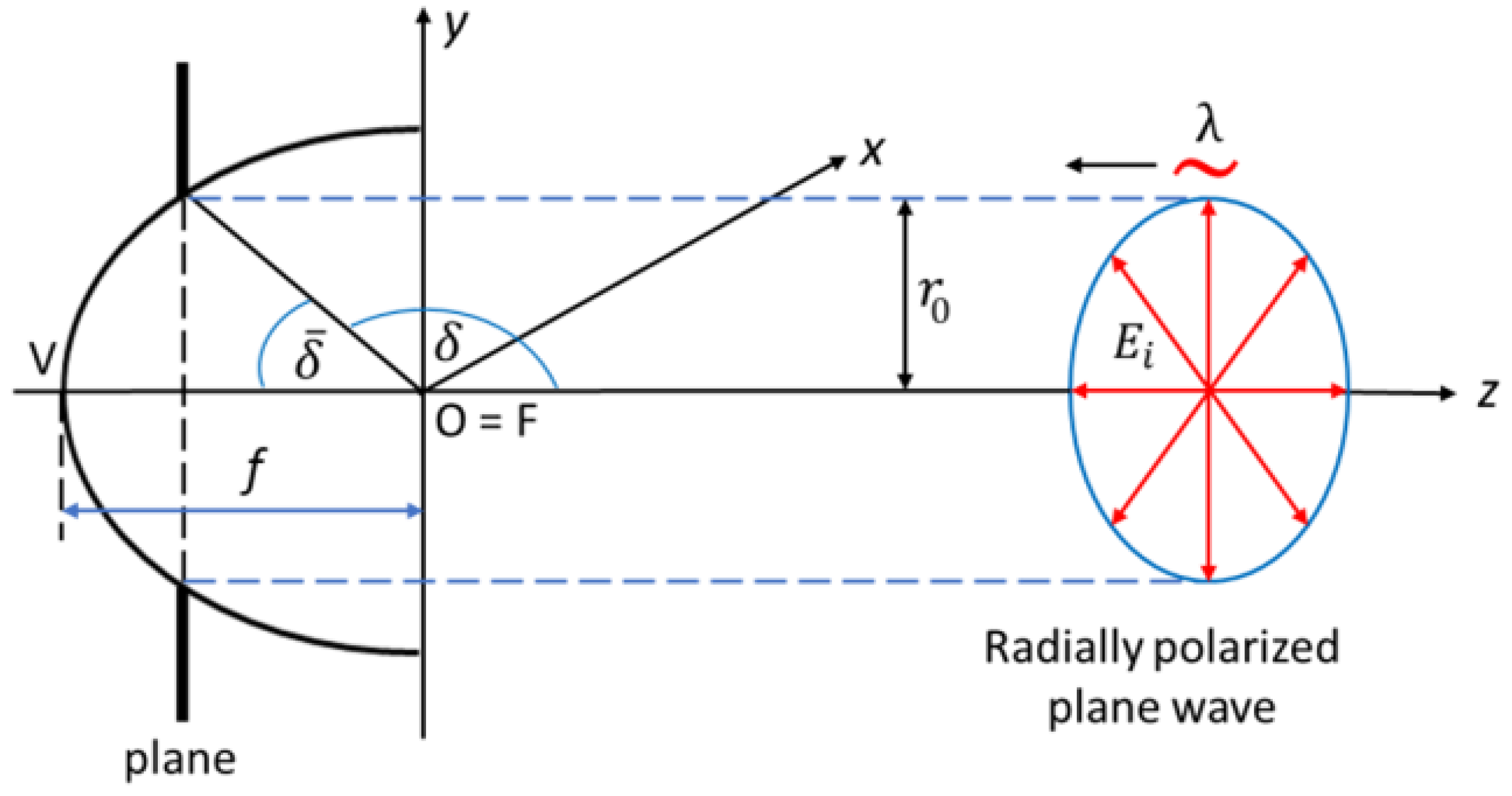
To derive an expression for the electric field focused by a segment of a parabolic mirror, we suppose that the segment of the paraboloid is limited by the apex V and a plane perpendicular to the optical axis positioned at z ≤ 0, as shown in Figure 2. The focusing angle δ, for which π/2 ≤ δ < π, determines the segment of the paraboloid [11].

We use the Stratton–Chu integral formula to derive an expression for the electric field upon focusing by a segment of a parabolic mirror [10].

$$\mathbf{E}\left(P\right)=\frac{1}{4\pi }{\int }_S\left[ik\left(\mathbf{n}\times \mathbf{H}\right)G+\left(\mathbf{n}\times \mathbf{E}\right)\times \nabla G+\left(\mathbf{n}·\mathbf{E}\right)\nabla G\right]\mathrm{d}A+\frac{1}{4\pi ik}{\oint }_C\nabla G\left(\mathbf{H}·\mathrm{d}\mathbf{s}\right),$$

(9)

with

$$G\left(u\right)=\frac{\mathrm{e}\mathrm{x}\mathrm{p}\left(iku\right)}{u},$$

(10)

where k = 2π/λ is wave number, λ is the wavelength of the incident beam and u is the distance between a point $\mathrm{S}\left(x_s,y_s,z_s\right)$ on the surface of the paraboloid and the observation point $\mathrm{P}\left(x,y,z\right)$. Hence,

$$u={\left[{\left(x_s-x\right)}^2+{\left(y_s-y\right)}^2{+\left(z_s-z\right)}^2\right]}^{1/2}={\left[{∆x}^2+{∆y}^2{+∆z}^2\right]}^{1/2}.$$

(11)

The first integral in Equation (9) represents the surface term, whereas the second integral represents the contour term, respectively.

∇G should be calculated at the points $\mathrm{S}\left(x_s,y_s,z_s\right)$ of the paraboloid [11]. It can be expressed as:

$$\nabla G\left(u\right)=ik\left(1-\frac{1}{iku}\right)\frac{G\left(u\right)}{u}\left(∆x{\mathbf{e}}_x+∆y{\mathbf{e}}_y+∆z{\mathbf{e}}_z\right).$$

(12)

The surface element of the paraboloid dA is given by:

$$\mathrm{d}A={\left[1+{\left(\frac{\partial z_S}{\partial x_S}\right)}^2+{\left(\frac{\partial z_S}{\partial y_S}\right)}^2\right]}^{1/2}\mathrm{d}{x}_S\mathrm{d}{y}_S=\frac{{{\rho }_s}^2}{n_z}\sin {\theta }_s\mathrm{d}{\theta }_s\mathrm{d}{\varnothing }_s.$$

(13)

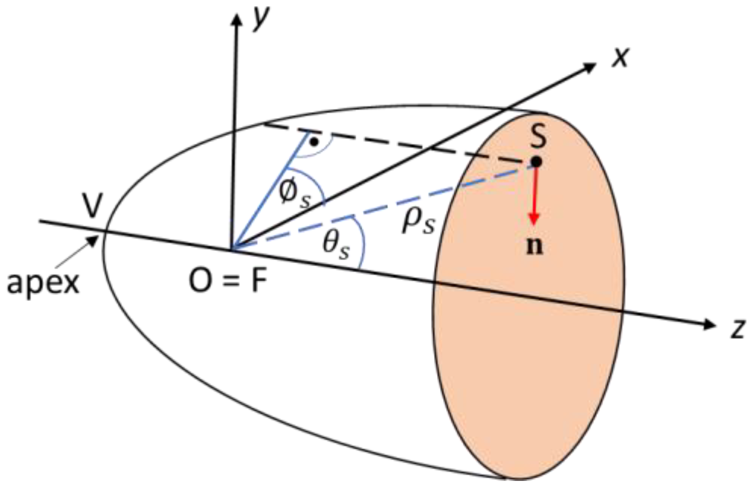
To determine the electric field created upon focusing by a segment of the parabolic mirror, we assume that the radially polarized incident monochromatic plane wave propagates in the negative z direction. Considering the cylindrical coordinate system (ρ, $\varnothing$, z), the radially polarized wave has an electric field in the radial direction with respect to the propagation axis while the magnetic field is aligned in the azimuthal orientation. There are no longitudinal components of the electric and magnetic fields. The incident electromagnetic field can be written as:

$$\begin{gathered} {\mathbf{E}}_i=a\mathrm{e}\mathrm{x}\mathrm{p}\left(-ikz\right)\left[\cos \varnothing {\mathbf{e}}_x+\sin \varnothing {\mathbf{e}}_y\right], \\ {\mathbf{H}}_i=a\mathrm{e}\mathrm{x}\mathrm{p}\left(-ikz\right)\left[\sin \varnothing {\mathbf{e}}_x-\cos \varnothing {\mathbf{e}}_y\right]. \end{gathered}$$

(14)

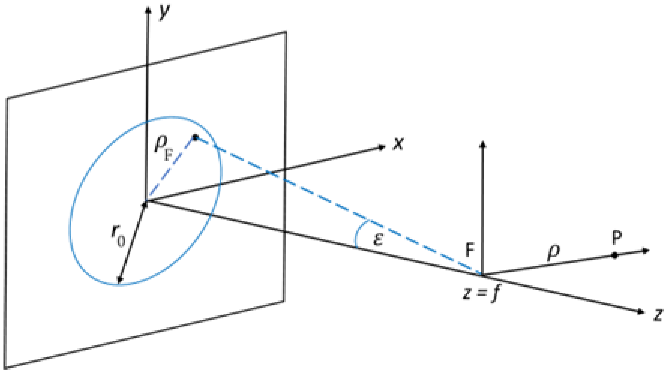
First, we discuss the surface integral in Equation (9). Using Equations (8) and (14), we can write quantities in Equation (9) as:

$$\begin{gathered} \mathbf{n}\times \mathbf{H}=2a{n}_z\left[\cos {\varnothing }_s{\mathbf{e}}_x+\sin {\varnothing }_s{\mathbf{e}}_y-\left(\frac{n_x}{n_z}\cos {\varnothing }_s+\frac{n_y}{n_z}\sin {\varnothing }_s\right){\mathbf{e}}_z\right]\mathrm{e}\mathrm{x}\mathrm{p}\left(-ik{z}_s\right), \\ \mathbf{n}\times \mathbf{E}=0, \\ \mathbf{n}·\mathbf{E}=2a\left(n_x\cos {\varnothing }_s+n_y\sin {\varnothing }_s\right)\mathrm{e}\mathrm{x}\mathrm{p}(-ik{z}_s). \end{gathered}$$

(15)

Substituting Equations (2), (10), (12), (13) and (15) into (9), we obtain the surface integral part in Equation (9):

$$\begin{gathered} {{\mathbf{E}}_S\left(\mathrm{P}\right)=\mathbf{E}}_S\left(\rho ,z\right)=a\frac{\mathrm{e}\mathrm{x}\mathrm{p}\left(2ikf\right)}{2\pi }ik\underset{\delta }{\overset{\pi }{\int }}\underset{0}{\overset{2\pi }{\int }}\mathrm{d}{\theta }_s\mathrm{d}{\varnothing }_s\frac{\mathrm{e}\mathrm{x}\mathrm{p}\left[ik\left(u-{\rho }_s\right)\right]}{u}{{\rho }_s}^2\sin {\theta }_s \\ \times \left\{\left[\cos {\varnothing }_s-\cot \left(\frac{{\theta }_s}{2}\right)\left(1-\frac{1}{iku}\right)\frac{∆x}{u}\right]{\mathbf{e}}_{\rho }+\cot \left(\frac{{\theta }_s}{2}\right)\left[1-\left(1-\frac{1}{iku}\right)\frac{∆z}{u}\right]{\mathbf{e}}_z\right\}, \end{gathered}$$

(16)

where $∆x={\rho }_s\sin {\theta }_s\cos {\varnothing }_s-\rho$, $∆z={\rho }_s\cos {\theta }_s-z$ and $u={\left[{∆x}^2{+∆z}^2\right]}^{1/2}$. P was supposed to lie on the x axis (see Figure 3). Due to the axial symmetry, ${\mathbf{E}}_S\left(\mathrm{P}\right)$ has no azimuthal component.

Now, we discuss the contour integral in Equation (9). According to Equation (4) and using the geometry shown in Figure 1 and Figure 2, the small vector line element on the circumference of the paraboloid is given by:

$$\mathrm{d}\mathbf{s}=2f\cot \left(\frac{\delta }{2}\right)\left(-\sin {\varnothing }_s{\mathbf{e}}_x+\cos {\varnothing }_s{\mathbf{e}}_y\right)\mathrm{d}{\varnothing }_s.$$

(17)

From Equations (5), (8) and (14), the Cartesian coordinate components $\left(H_x,H_y,H_z\right)$ of the total magnetic field can be written as:

$$\begin{gathered} H_x=2a\sin {\varnothing }_s\mathrm{e}\mathrm{x}\mathrm{p}\left(-ikz\left(\delta \right)\right), \\ {H}_y=-2a\cos {\varnothing }_s\mathrm{e}\mathrm{x}\mathrm{p}\left(-ikz\left(\delta \right)\right), \\ {H}_z=0. \end{gathered}$$

(18)

Hence:

$$\mathbf{H}·\mathrm{d}\mathbf{s}=-4af\cot \left(\frac{\delta }{2}\right)\mathrm{e}\mathrm{x}\mathrm{p}\left(-ikz\left(\delta \right)\right)\mathrm{d}{\varnothing }_s.$$

(19)

Substituting Equations (10), (12) and (19) into (9), we obtain the contour integral part in Equation (9):

$$\begin{gathered} {\mathbf{E}}_C\left(\mathrm{P}\right)={\mathbf{E}}_C\left(\rho ,z\right)=-\frac{af\mathrm{e}\mathrm{x}\mathrm{p}\left(2ikf\right)}{\pi }\cot \left(\frac{\delta }{2}\right){\int }_0^{2\pi }\frac{\mathrm{e}\mathrm{x}\mathrm{p}\left[ik\left(u-\rho \left(\delta \right)\right)\right]}{u} \\ \times \left(1-\frac{1}{iku}\right)\left(\frac{∆x}{u}{\mathbf{e}}_{\rho }+\frac{∆z}{u}{\mathbf{e}}_z\right)\mathrm{d}{\varnothing }_s, \end{gathered}$$

(20)

With $∆x={\rho }_s\left(\delta \right)\sin \delta \cos {\mathrm{\varnothing }}_s-\rho$, $∆z={\rho }_s\left(\delta \right)\cos \delta -z$ and $u={\left[{∆x}^2{+∆z}^2\right]}^{1/2}$. Due to the axial symmetry, ${\mathbf{E}}_C\left(\mathrm{P}\right)$ has no azimuthal component.

The total complex electric field can be given as:

$$\mathbf{E}\left(\rho ,z\right)={\mathbf{E}}_S\left(\rho ,z\right)+{\mathbf{E}}_{\mathrm{C}}\left(\rho ,z\right).$$

(21)

We would like to call attention to the fact that in the following section, $E$_ρ and $E$_z represent the real parts of the complex field components.

4. Applications of the Theoretical Results for Different Focusing Conditions

To provide useful information for specialists who would like to apply the tightly focused field, we present and discuss some results of calculations using the previously introduced vector diffraction theory for various focusing geometries. Parabolic mirrors are standard devices in optical setups and are especially used at wavelength ranges (e.g., terahertz = THz) where conventional lenses and spherical mirrors fail. For the sake of generality, instead of specifying the focal length (f), the wavelength (λ) and r₀ (that can be interpreted as the incident beam radius, see Figure 2) as absolute parameters, we introduce the λ/f and r₀/f as relative parameters. This latter relates to the $\delta$ focusing angle (see Figure 2) as

$$\delta =\mathrm{a}\mathrm{r}\mathrm{c}\mathrm{c}\mathrm{o}\mathrm{s}\left(\frac{\frac{1}{4}{\left(\frac{r_0}{f}\right)}^2-1}{\frac{1}{4}{\left(\frac{r_0}{f}\right)}^2+1}\right),$$

(22)

and

$$\overline{\delta }=\pi -\delta$$

(23)

During the analysis, λ/f was kept below 0.1, since the λ/f > 0.1 case has less practical relevance. Supposing a typical value of f = 50 mm, the λ/f < 0.1 condition holds not only for the visible and (near-, mid-) infrared, but also for the THz frequency range (0.1–10 THz). Even in the case of λ/f = 0.1, the corresponding frequency is only 0.06 THz, so for λ/f > 0.1 the whole THz range is covered. The importance of the THz fields is outstanding due to their applicability for particle acceleration [17,18,19] because of their advantageous wavelength and because of the availability of pulses with extremely high pulse energies and electric field strengths owing to the tilted-pulse-front technique [20,21].

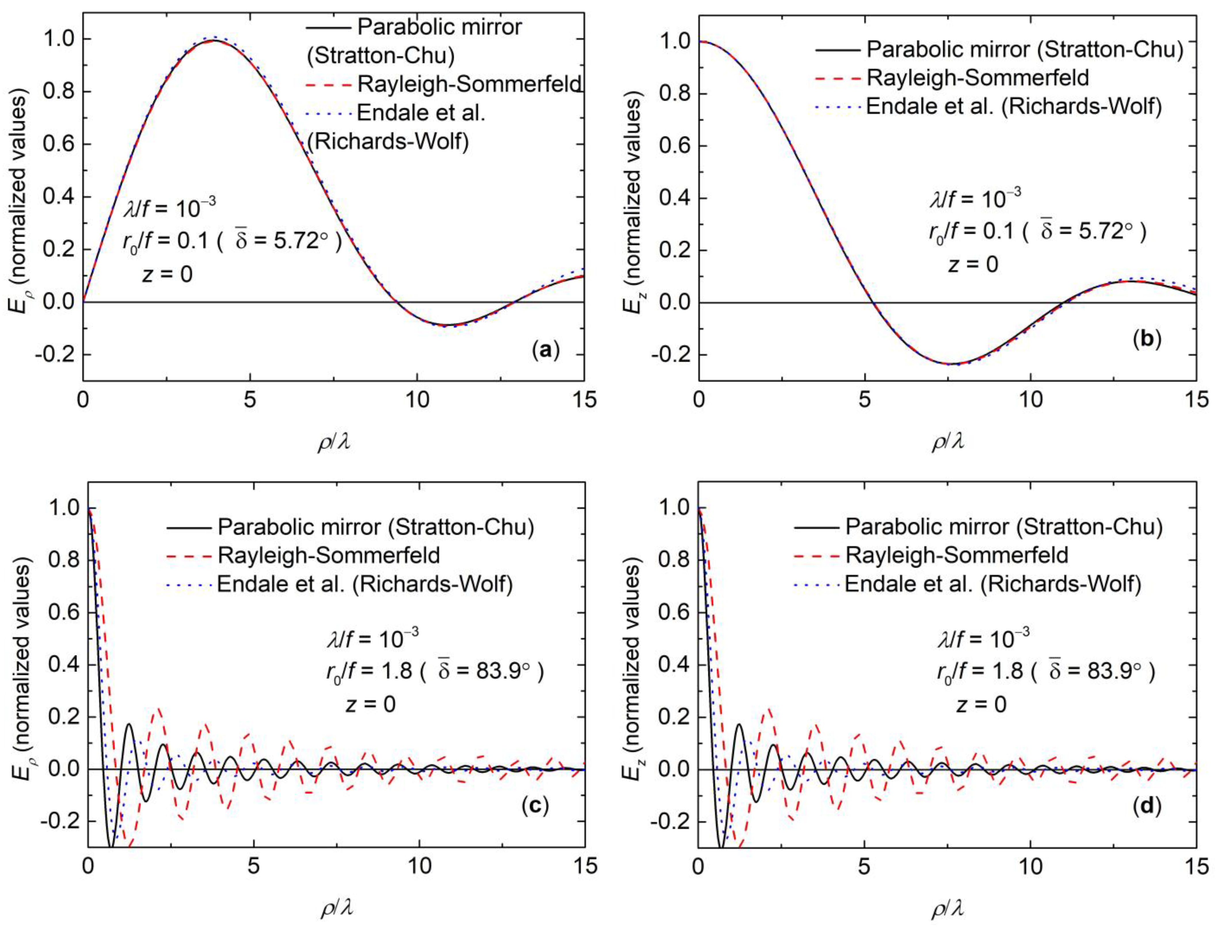
Before applying our above introduced theory based on the Stratton–Chu formulae, we must confirm its reliability. Therefore, as a validation, we compare its results with those of the commonly known scalar diffraction methods by treating separately two perpendicular (x and z) polarization components. The $E$_ρ and $E$_z field components determined with scalar diffraction methods (red, dashed curves in Figure 4) were deduced from the Rayleigh–Sommerfeld diffraction formula [22] adapted for the case shown in Figure 3 supposing a ‘thin’ focusing element. The amplitudes of the aperture functions belonging to the transversal and longitudinal field components just leaving the focusing element are

$$\begin{gathered} {E_{F\rho }=E}_0\cos \mathsf{\epsilon }\cos {\varnothing }_F=E_0\frac{f}{\sqrt{{{\rho }_F}^2+f^2}}\cos {\varnothing }_F, \\ {E_{Fz}=E}_0\sin \mathsf{\epsilon }=E_0\frac{{\rho }_F}{\sqrt{{{\rho }_F}^2+f^2}} \end{gathered}$$

(24)

respectively, where $E_0$ is the electric field just before reaching the focusing element. The radially dependent part of the phase factor resulting from the focusing element is

$$\mathrm{e}\mathrm{x}\mathrm{p}\left(-i{\phi }_F\right)=\mathrm{e}\mathrm{x}\mathrm{p}\left(-ik\frac{{{\rho }_F}^2}{2f}\right).$$

(25)

Hence

$$\begin{gathered} E_{\rho }\left(\rho \right)\propto \underset{0}{\overset{r_0}{\int }}\underset{0}{\overset{2\pi }{\int }}{E}_{F\rho }\mathrm{e}\mathrm{x}\mathrm{p}\left(-i{\phi }_F\right)\frac{\exp \left(-iku\right)}{u^2}{\rho }_F\mathrm{d}{\rho }_F\mathrm{d}{\varnothing }_F, \\ {E}_z\left(\rho \right)\propto \underset{0}{\overset{r_0}{\int }}\underset{0}{\overset{2\pi }{\int }}{E}_{Fz}\mathrm{e}\mathrm{x}\mathrm{p}\left(-i{\phi }_F\right)\frac{\exp \left(-iku\right)}{u^2}{\rho }_F\mathrm{d}{\rho }_F\mathrm{d}{\varnothing }_F, \end{gathered}$$

(26)

with

$$u={\left({{\rho }_F}^2+f^2+{\rho }^2-2\rho {\rho }_F\cos {\varnothing }_F\right)}^{\frac{1}{2}}.$$

(27)

We also determine the electric field distributions by using the formula of Endale et al. [13] for the case of a flat-top beam. This model is based on the diffraction theory of Richards–Wolf [9]. The curves computed this way are plotted by blue, dotted lines in Figure 4.

For parameters of λ/f = 10⁻³ and r₀/f = 0.1 (with corresponding $\overline{\delta }={5.72}^{\mathrm{o}}\mathrm{a}\mathrm{n}\mathrm{g}\mathrm{l}\mathrm{e}$), the contour term in our model is negligible beside the surface term. Furthermore, the parabolic mirror can be considered to be thin. In this paraxial regime, a particularly good agreement can be found between the results of our (Stratton–Chu) and the other two (Rayleigh–Sommerfeld, Richards–Wolf) models, as seen in Figure 4a,b.

For λ/f = 10⁻³ and for large numerical aperture (r₀/f = 1.8 with corresponding $\overline{\delta }={83.9}^{\mathrm{o}}\mathrm{a}\mathrm{n}\mathrm{g}\mathrm{l}\mathrm{e}$), the Rayleigh–Sommerfeld integral leads to a misleading result. Even the model of Endale et al. [13] (which is not restricted to small numerical apertures) works well only at the vicinity of the z axis, for low ρ/λ values.

These conclusions confirm the necessity of the use of our model in large numerical aperture regimes, when the spatial extension of the parabolic mirror in the z (longitudinal) direction becomes comparable with its transversal extension.

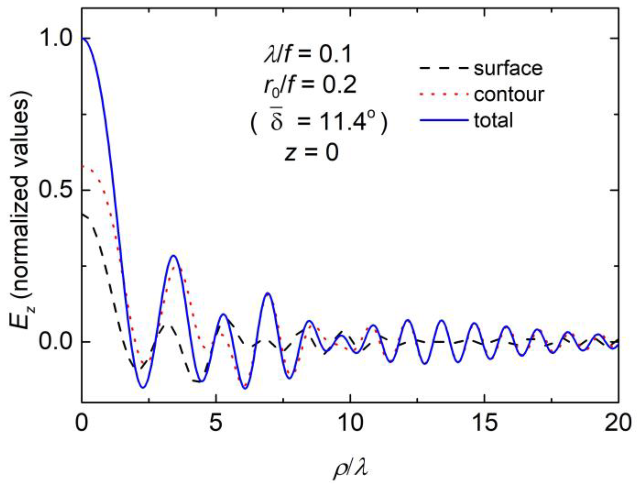
The contribution of the contour term is negligible in all cases examined in the following. However, for example in the case of r₀/f = 0.2 and λ/f = 0.1, the surface and the contour terms have the same orders of magnitude, as illustrated in Figure 5. Here, the black dashed line belongs to the surface and the red dotted line to the contour term, while the blue solid line represents their sum, the total $E$_z field component. Under the focusing conditions of Figure 5 for the case of the $E$_ρ field component, the surface term dominates over the contour term.

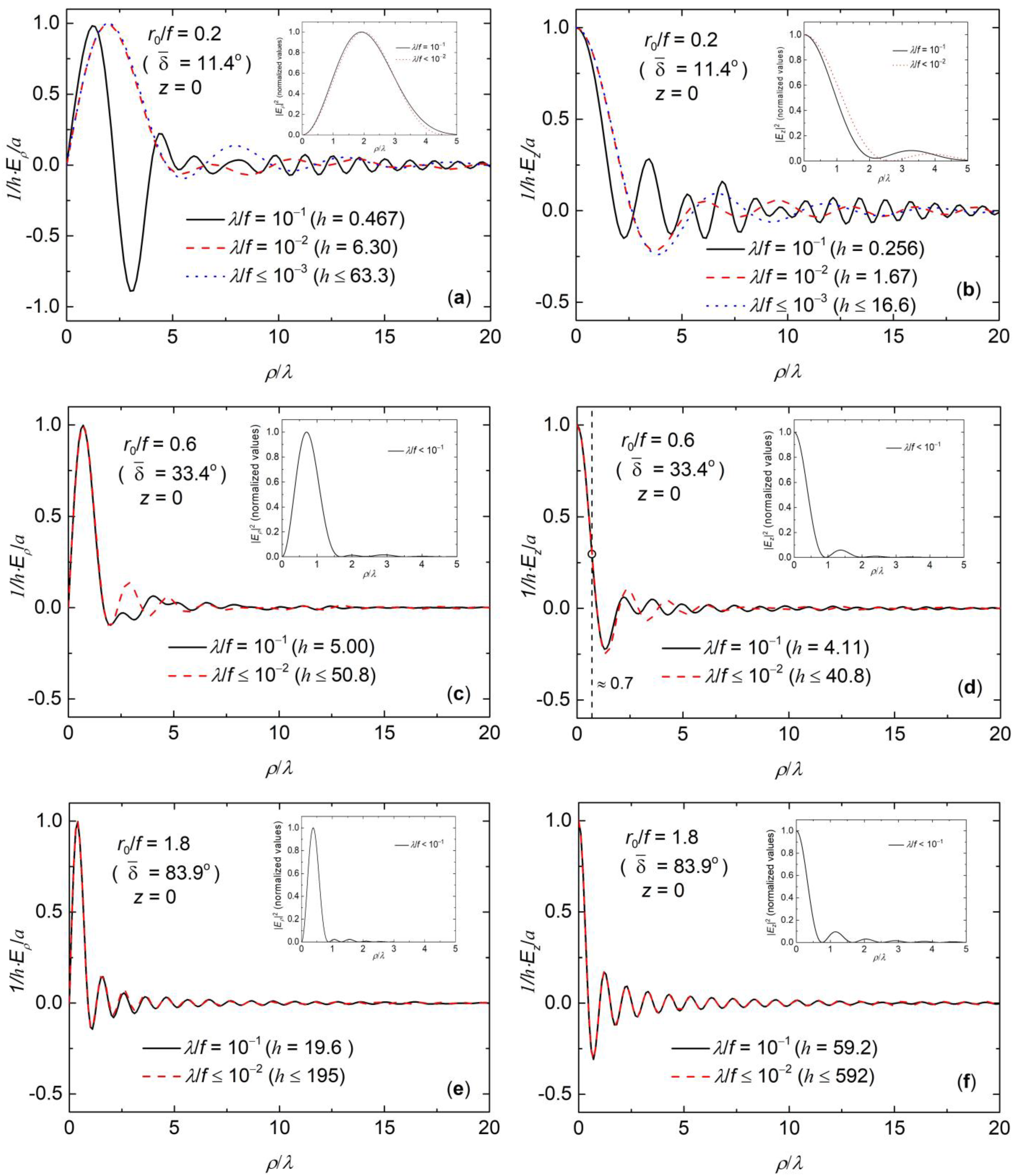
In Figure 6, the normalized $E$_ρ and $E$_z distributions are plotted versus the radial coordinate normalized by the wavelength. This coordinate normalization makes it comfortable to plot the curves with different λ/f values on the same scale. Figure 6a,b belong to r₀/f = 0.2 ($\overline{\delta }$ = 11.4°), Figure 6c,d to r₀/f = 0.6 ($\overline{\delta }$ = 33.4°) and Figure 6d,e to r₀/f = 1.8 ($\overline{\delta }$ = 83.9°). All curves of Figure 6 belong to the focal plane (z = 0). All curves are normalized to 1. However, in the graphs in brackets, one can find the field amplitude enhancement factors, $h$, relative to the amplitude of the incoming field, $a,$ in order to provide information on how the magnitude of the field components scale with the r₀/f and λ/f parameters, making it possible to compare the $E$_ρ and $E$_z amplitudes in case of a given focusing geometry.

All the curves of Figure 6 oscillate with decaying amplitude. At the focal point, $E$_z has maxima, while $E$_ρ is zero in each case, as expected. It was found that for the fixed r₀/f value, the curves of different wavelengths could not be practically distinguished from each other below a threshold λ/f. These identical curves are indicated by the “≤” sign (see the labels). The threshold λ/f value increases with increasing r₀/f.

From analyzing the enhancement factors (shown in the brackets), it is obvious that at constant r₀/f the field strength increases with the decreasing wavelength. According to detailed calculations, below the threshold it scales with λ⁻¹. If the wavelength is taken to be fixed, the field strength strongly increases with increasing r₀/f, as expected. Comparing the amplitudes of curves with the same λ/f in Figure pairs Figure 6a,b, Figure 6c,d, Figure 6e,f, it is obvious that for the low value of r₀/f (Figure 6a,b), the $E$_ρ field component is larger than E_z, while for large r₀/f (Figure 6e,f) the E_z is dominant, as expected intuitively. This analysis is especially interesting for those who plan particle acceleration applications. It is also seen in Figure 6 that the first zero crossing value decreases with increasing r₀/f for both field components.

To more easily follow some characteristics, we plotted in the insets the absolute value of squared field components. The first maxima for the radial component and the first minima for both components shift to the left with increasing r₀/f, although the degree of this shift decreases for larger r₀/f.

Results like the ones shown in Figure 6 are needed when a waveguide-based electron accelerator is designed. If the aim is the efficient in-coupling into the waveguide by focusing, one should match the width (in ρ/λ) of the E_z distribution curve to the characteristic r₁/λ value of the waveguide, where r₁ is the core radius. For the optimized parameters (r₁ = 380 µm core radius, d = 32 µm dielectric thickness, 0.6 THz frequency) of a dielectric coated metallic waveguide, r₁/λ ≈ 0.7 [23]. Among the curves of Figure 6, the best agreement can be found in Figure 6d. This means that r₀/f ≈ 0.6 can be an appropriate focusing geometry for in-coupling into the waveguide.

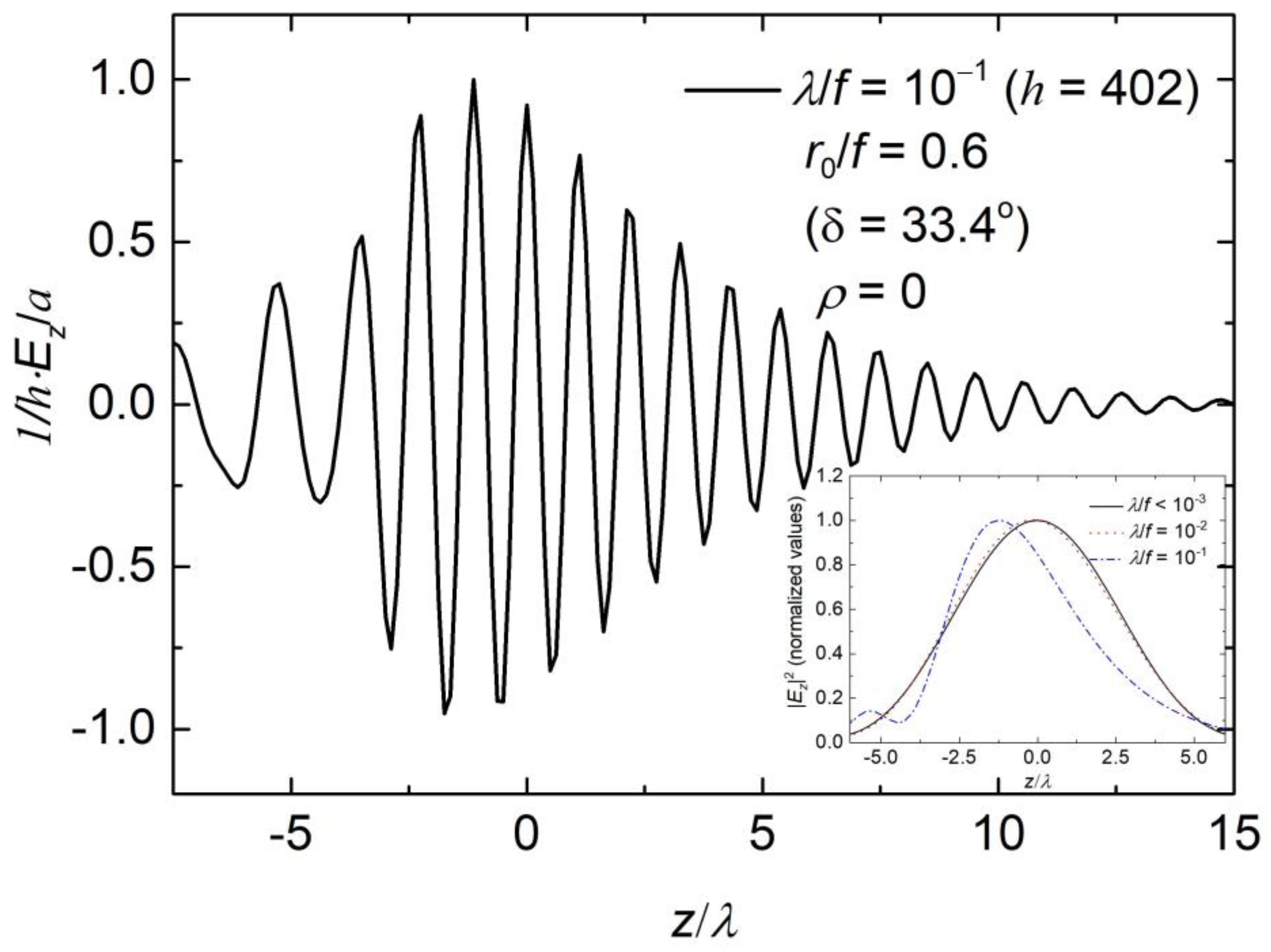
It is important to obtain information on the longitudinal distributions as well. As an example, the distribution of E_z along the optical axis was computed and plotted in Figure 7 for λ/f = 0.1 and r₀/f = 0.6. It is clear from the graph that the peak of the curve is shifted from the focus towards the apex of the mirror, as already observed for the case of linear polarization [11]. The λ/f dependence of this shifting effect can be studied more clearly on the |E_z|² curves (inset). Below λ/f = 10⁻² this shift is negligible, while for λ/f = 10⁻¹ the shift of the peak of the |E_z|² curve is ~1.2 λ. The FWHM of the |E_z|² curve is ~4.5 λ for λ/f = 10⁻¹ and ~6 λ for λ/f ≤ 10⁻². Examinations showed that for fixed λ/f, the shift is larger for lower r₀/f values.

5. Conclusions

In this paper, based on the Stratton–Chu integral we derived general formulae to be used when a radially polarized electromagnetic wave is focused by a parabolic mirror with perfect reflectance. The theory was successfully validated within the limit of a small numerical aperture and negligible contour term when the Rayleigh–Sommerfeld diffraction formula served as a reliable alternative. We determined and analyzed the transversal and the longitudinal distribution of the radial and longitudinal electric field components for various focusing conditions. Our results can be interesting in the THz techniques, like THz imaging, linear and nonlinear THz spectroscopy, and especially for particle acceleration applications, where an intense longitudinal electric field is a requirement. Our work focused on monochromatic plane waves and simply connected paraboloid segments in on-axis geometry. But it can be further developed for the case of electromagnetic pulses, for the case of various input beams (e.g., vector Gaussian beam) and for various types of parabola segments (e.g., ring-like slice or off-axis geometry).