Article

Angle-Dependent Transport Theory-Based Ray Transfer Function for Non-Contact Diffuse Optical Tomographic Imaging

by
Stephen Hyunkeol Kim
1,2,*,†,
Jingfei Jia
3,† and
Andreas H. Hielscher
1,*
1
Department of Biomedical Engineering, New York University, New York, NY 10010, USA
2
Department of Radiology, New York University, New York, NY 10016, USA
3
Department of Biomedical Engineering, Columbia University, New York, NY 10027, USA
*
Authors to whom correspondence should be addressed.
These authors contributed equally to this work.
Photonics 2023, 10(7), 767; https://doi.org/10.3390/photonics10070767
Submission received: 1 May 2023 / Revised: 26 June 2023 / Accepted: 1 July 2023 / Published: 3 July 2023

Abstract

:
This work presents a generalized angle-dependent ray transfer function that can accurately map the angular and spatial distribution of light intensities on the tissue surface onto a camera image plane in a non-contact camera-based imaging system. The method developed here goes beyond existing ray transfer models that apply to angle-averaged tomographic data alone. The angle-dependent ray transfer operator was constructed using backward ray tracing based on radiation surface theory. The proposed method was validated using numerical phantoms and experimental data from an actual non-contact imaging system.

1. Introduction

Diffuse optical tomography (DOT) has increasingly been applied in many clinical areas, such as breast imaging [1,2,3], joint imaging [4,5,6], brain imaging [7,8], vascular imaging [9,10], and small animal imaging [11,12,13], through model-based image reconstruction algorithms [14,15,16], due to its non-ionizing radiation, portability, real-time imaging, and low instrumentation cost.
DOT systems have long relied on optical fibers to deliver and measure light over the tissue of interest. These fibers are typically in contact with the tissue [17,18,19]. This has often limited the number of detectors, thus restricting DOT image reconstruction’s spatial resolution. Furthermore, the fibers need to be rearranged according to the geometry of the object for every different experiment, which brings lots of inconveniences and may introduce very strong noise if any fiber does not well contact the tissue surface. In recent years, non-contact measurements involving so-called charged-coupled device (CCD) or complementary metal-oxide-semiconductor (CMOS) cameras have been explored to overcome these disadvantages. These approaches have shown significant advantages in detection sensitivity, image quality, and system simplicity [20,21,22,23]. In non-contact imaging, a way to model photon transport in free space, i.e., a measurement operator  Q  that projects the surface light distribution onto an image plane of the camera, is required, in addition to a model for light propagation inside the tissue. All proposed numerical algorithms [24,25] to simulate light propagation in tissue are very computationally expensive for the photon-transport process in free space. Fiber-based systems usually have a simpler measurement operator  Q  (i.e., equivalent to the partial current operator), but they can be cumbersome to use when handling complex geometries and may introduce higher measurement noise due to contact issues. To overcome these difficulties and achieve better performance, contact-free imaging systems are becoming more popular in the DOT. For these imaging systems, accurate modeling by the measurement operator  Q  is crucial for quality image reconstruction but is not as straightforward as for fiber systems. As a stochastic method, Monte-Carlo simulation [25,26,27] can handle this problem. However, many photons are needed for the simulations to obtain a reasonable result, leading to relatively low efficiency.
To overcome this problem, Ripoll et al. proposed an efficient free-space light transport model [20] that does not employ statistical MC methods. Instead, they compute an integral of light intensity for every point on the focal plane over the directions that can lead the photon to the aperture through that point. Based on this model, Schulz et al. proposed a simplified model [21] using the perspective projection method by replacing the camera lens with a virtual pinhole. In 2009 and 2010, Chen et al. published two improved models [28,29] based on the hybrid radiosity-radiance theorem. The influence of the camera lens was analyzed with the thin lens assumption in both models. In addition, the radiometric vignetting coefficient [30] and generalized rectangular central obscuration [31] were also studied as factors that impact the performance evaluation of realistic imaging instrument design.
Yet, existing models so far still have two major limitations. First, they do not fully consider the angular dependency of the light intensity in the model, so they only work in the limit of the diffusion equation (DE). It should be noted that angularly resolved measurement data substantially improves both localization and quantification accuracy of radiative transfer equation (RTE)-based DOT reconstruction [32]. Second, they do not take additional optical elements that are typically used into account. An optical system, such as a mirror system or lens group, is often placed between the object and the CCD camera to gather more information on the surface light intensity distribution. The lack of consideration for such cases also limits the application of the research mentioned above in practice.
To overcome these problems, a distributed-backward-ray-tracing model is proposed here to simulate the photon transport process in free space. In this model, pseudo photons are shot from the CCD chip and transported back to the object’s surface. In this way, a mapping is established between the angular-dependent photons on the object’s surface and those on the detector of the CCD camera. Furthermore, a coordinate transformation is applied to convert the integral over the solid angle on the object surface to an integral over the solid angle on the CCD chip. The determinant of the transformation Jacobian matrix is estimated with the perturbation method. With this model, the contribution of photons from different surface locations and directions to signals received on the CCD camera can be expressed as a linear operator, which is required for formulating the optimization problem in DOT. The proposed model fully considers the angular dependency of light intensity and thus can be applied in RTE-DOT, which provides higher accuracy in many cases. Moreover, this proposed model could handle photon transport problems with a general optical system between the object and the CCD camera to collect more signals, which are often limited by the size of the aperture. That can greatly improve the performance of receiving photons from more perspectives. Thus, it is reasonable to expect a better performance and a more reliable result in non-contact DOT with this proposed model.
The remainder of this paper is organized as follows. The detailed derivation of the novel backward ray-tracing algorithm is given in Section 2. This model is then validated with numerical experiments and reconstruction results in Section 3. This work finally concludes with a discussion in Section 4.

2. Material and Methods

The basic concept for DOT imaging is to find a spatial distribution of optical properties inside the medium that minimizes the difference between model predictions  P  and measurements  z  at detector locations as,
min x 1 2 P z 2
where  x  is the optical property that is to be reconstructed and  ψ  is the light intensity distribution within the imaging object. Here, the prediction  P  can be described as a linear functional of radiative light intensity distribution  ψ  and measurement operator  Q  as given by  P = ψ Q . In non-contact DOT systems, Q is the mapping between radiative light intensity distribution and camera pixel measurement. Therefore, the construction of Q requires a theory of surface radiation and light propagation in free space, especially between surfaces, and how the radiant power can be evaluated on each surface element.

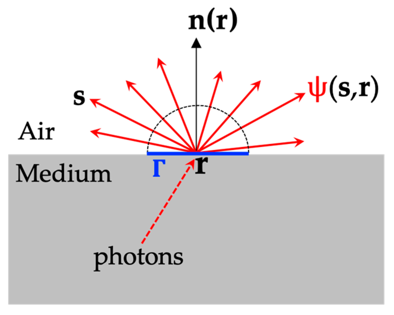
2.1. Surface Radiation Theory

According to the knowledge of surface radiation theory [33,34], once the radiative light intensity distribution  ψ ( r , s )  [ W / mm 2 / sr ] in an object  O  has been already given, the total emission power of  P surf  [W] on a small area  Γ  on its surface  O  as shown in Figure 1, can be given by
P surf Γ = Γ 2 π ψ r , s 1 R s n r s n r d s   d r ,
where  r  is a position vector that indicates the location on the surface of the object;  s  and  n ( r )  are two-unit vectors that represent the photon’s propagation direction and the outgoing normal vector on the surface respectively, where the normal vector is a function of the location;  R  represents the reflectivity on the tissue-air boundary.
As shown in Figure 1, the surface can emit light in infinitely many directions, and light intensity has different strengths in different directions and also in different fields of view. The solid angle is a measure of the amount of the field of view that is covered by a surface or object at a particular point. When an infinitesimal surface  dA  is seen from a point  P , the infinitesimal solid angle  d Ω  is defined as the projection of the surface onto a plane normal to the direction vector, divided by the square of the distance  S  between  dA  and  P , as given by  d Ω = dA / S 2 , and it is measured in steradians [sr]. If the surface is projected onto the unit hemisphere above the point, the solid angle is equal to the projected area itself. Thus, an infinitesimal solid angle is simply an infinitesimal area on a unit sphere, or  d Ω = sin θ d θ d ψ  on a spherical coordinate.
Therefore, the infinitesimal power  dP r ,   s  that emits from the infinitesimal solid angle  d Ω  constructed around the direction  s  centered at    r  is given by
dP surf r ,   s = ψ r ,   s 1     R s n r s n r d s d r ,   r     Γ .
To use Equation (3) numerically, we express the vector  r  and  s  with a parametric coordinate system. The direction vector  s  is commonly represented by the spherical coordinate system.
s = s ( θ ,   φ ) : = sin θ cos φ , sin θ sin φ , cos θ .
Since the location vector  r  in (3) is on a local piece  Γ  of a 2D manifold  O , it is convenient to parameterize it by a locally differentiable parametric equation with two free parameters  λ 1 ,   λ 2 ,
r = r λ 1 ,   λ 2 .
Options for  λ 1  and    λ 2  are not unique. However, the tetrahedron mesh discretization discretizes the object surface with triangle elements correspondingly (see a cylinder example in Figure 2a). It is natural to assume  Γ  is a triangle element on the surface (See Figure 2b) and to consider the parametric coordinate system for  r     Γ .
Here the 2D barycentric coordinate system [35] (also called the areal coordinates system) is briefly introduced. Assuming the location vectors of the three vertices of the host triangle element are  r A r B , and  r C , we define three vectors  v AB : =   r B     r A v AC : =   r C   r A  and  v   : =   r     r A  (See Figure 2b). Therefore, equation  v = λ 1 v AB + λ 2 v AC  has a unique pair of solution  λ 1 ,   λ 2  and it is used as  r ’s local parametric coordinates. This coordinate system leads to a straightforward expression of  r λ 1 ,   λ 2 , which is given by
r λ 1 , λ 2 : =   λ 1 v AB + λ 2 v AC + r A .
Another benefit of this coordinate system is that the normal vector  n  is a constant and does not depend on the location  r  within  Γ . Therefore, according to (4) and (6), we have
n d r = r / λ 1   ×   r / λ 2 d λ 1 d λ 2 = 2 Γ d λ 1 d λ 2 , s d s = sin θ s d φ d θ ,
where  Γ  is the area of triangle element  Γ  and can be pre-calculated after the mesh generation.
.
With (7), we can construct a four-dimensional coordinate system to express the angularly dependent light intensity on  A  and the infinitesimal power  dP Γ  in (3) can be given by
dP surf Γ = Ω r ( Γ )   ×   Ω s ( Γ ) q surf λ 1 , λ 2 , φ , θ d φ d θ d λ 1 d λ 2 ,
where  Ω r ( Γ )  and  Ω s ( Γ )  represents the feasible set for location vector  r  and direction vector  s  under this coordinate system,
Ω r Γ : = λ 1 , λ 2 :   r λ 1 , λ 2     Γ ,   Ω s Γ : = φ , θ :   s φ , θ n Γ   >   0 .
q surf λ 1 ,   λ 2 ,   φ ,   θ  is the power density function on the surface under this coordinate system, which is given by
q surf λ 1 ,   λ 2 ,   φ ,   θ = 2 sin θ Γ 1 R s n ψ r , s .
In practice,  ψ r ,   s  is solved with discretized forward solvers, thus it is only available for the triangle vertices  r A ,   r B ,   r C  and for certain solid angles  s i i = 1 N SA , so we can approximate  ψ r ,   s  for any    s  and  r     Γ  with the linear interpolation in the spatial domain and the nearest neighbor method in the solid angle domain.
ψ r λ 1 ,   λ 2 ,   s     1     λ 1     λ 2 ψ r A ,   s + λ 1 ψ r B ,   s + λ 2 ψ r C ,   s
          1     λ 1     λ 2 ψ r A ,   s k + λ 1 ψ r B ,   s k + λ 2 ψ r C ,   s k ,
where  k = argmin k s s k .

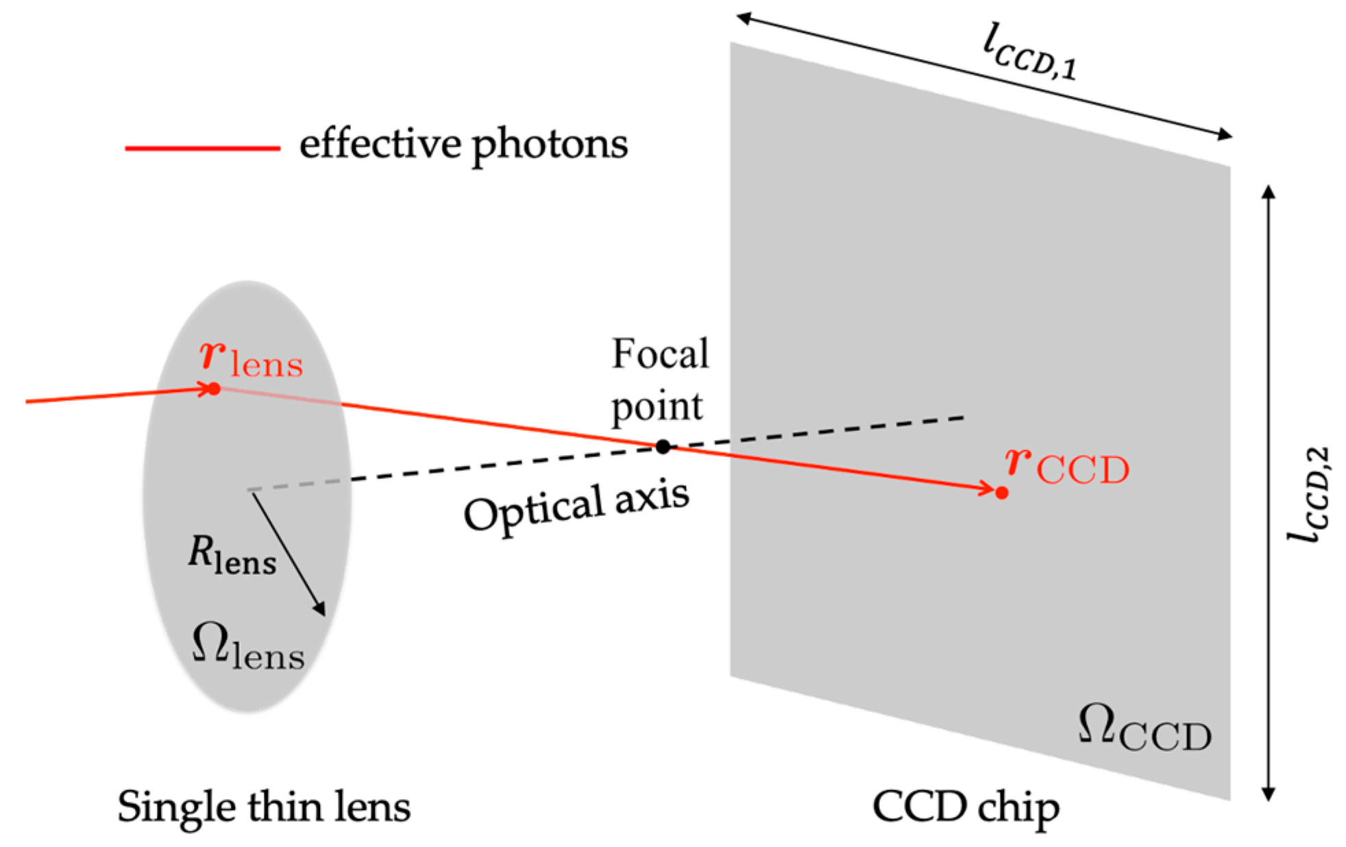
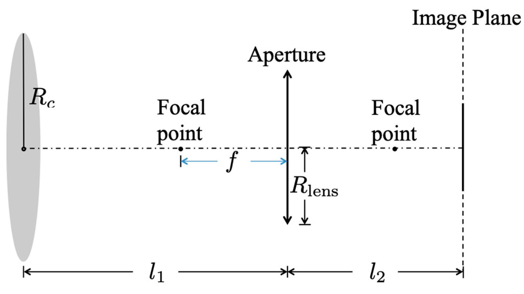
2.2. CCD Camera Acceptance Coordinates System

To reduce the complexity of the model, the CCD camera is assumed to only consist of a single thin lens  Ω lens  (the aperture) with a radius as  R lens   [ mm ]  and a CCD chip  Ω CCD  with size  l CCD , 1 mm   ×   l CCD , 2 mm  (See Figure 3). Under this assumption, the readings on the CCD chip are contributed by effective photons that pass through the aperture and finally reach the CCD chip after the refraction (the red solid arrow line in Figure 3). Any effective photon can be uniquely identified with two location vectors: (1)  r lens  defined as the intersection point between its optical path and  Ω lens  and (2)  r CCD  defined as its final position on  Ω CCD  (see Figure 3). Therefore, the total energy that is received by the CCD chip,  P CCD  [W], can be calculated with an integral over the light intensity  J r lens , r CCD  on  Ω lens   ×   Ω CCD ,
P CCD = Ω lens × Ω CCD J r lens ,   r CCD r CCD     r lens n CCD d r lens d r CCD ,
where  n CCD  is the normal vector of the CCD chip that points to the other side of  r lens .
Based on the circular shape of the aperture and the rectangular shape of the CCD chip, we represent  r lens  and  r CCD  with the polar coordinate system
r lens = r lens ρ ,   ω ,   0     ρ     R lens ,   0     ω   <   2 π , r CCD = r CCD x ,   y ,   0   x     l CCD , 1 ,   0     y     l CCD , 2   .
With this parametric expression, (12) can be written as
P CCD = 0 l CCD , 2 0 l CCD , 1 0 2 π 0 R lens q CCD ρ ,   ω ,   x ,   y d ρ d ω dxdy ,
where the energy density  q CCD ρ ,   ω ,   x ,   y   [ W / mm 3 / sr ]  under this coordinate system is to be calculated in the next section.

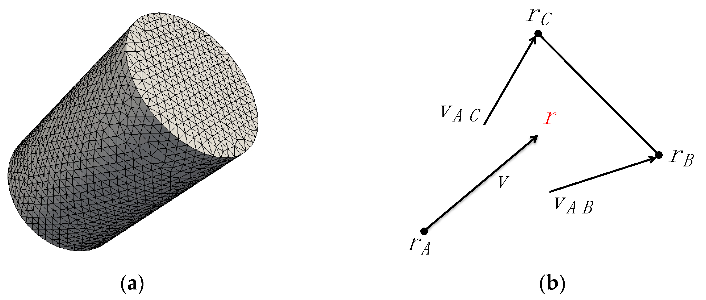
2.3. Light Propagation in Free Space and Coordinate Transformation

The status of any photon that emits from the object surface and is finally received by the CCD chip (also referred to as the effective photons) can be described with the coordinates  ρ ,   ω ,   x ,   y  or with a triangle element  Γ ,  and its corresponding ordinates  λ 1 ,   λ 2 ,   φ ,   θ . Therefore, we can define two sets based on these two coordinate systems to describe the status of effective photons.
S surf : = Γ , λ 1 , λ 2 , φ , θ :   photon   with   status   Γ , λ 1 , λ 2 , φ , θ   is   effective   , S CCD : = ρ , ω , x , y :   photon   with   status   ρ , ω , x , y   is   effective   .
Therefore, for any  Γ ,   λ 1 ,   λ 2 ,   φ ,   θ     S surf , we have  λ 1 ,   λ 2     Ω r Γ  and    φ ,   θ     Ω s Γ ; for any  ρ ,   ω ,   x ,   y     S CCD 0     ρ     R lens 0     ω   <   2 π 0     x     l CCD , 1  and  0     y     l CCD , 2  are satisfied. We can also consider  S surf  as the initial status set of effective photons since it characterizes the starting positions and directions. On the other hand,  S CCD  can be considered as the final status set of effective photons since it contains information on the CCD camera side.
In non-contact imaging, some optical systems, such as conical mirrors, are often employed to magnify the signal received by the CCD camera. To track the contribution of photons in the complex optical system, we represent the light propagation in free space with an operator  F , which maps from the initial status set  S surf  to its final status set  S CCD . In this work, the following assumptions are imposed on the operator  F :
  • The operator  F  is a one-to-one and deterministic function from  S surf  to  S CCD . Therefore, the light propagation operator  G   : =   F 1  is well defined.
  • The operator  F  is locally differentiable. In other words,  F Γ :   λ 1 ,   λ 2 ,   φ   , θ     ρ ,   ω ,   x ,   y , which is defined as  F  constrained on the surface triangle element  Γ , and its inverse  G Γ  are differentiable.
  • There is no energy loss during the light’s travel from the surface to the CCD chip.
These assumptions are not strong and are not satisfied by most of the general optical systems. Under these assumptions, we consider the total energy received from an infinitesimal unit volume  d ρ d ω dxdy  around  ρ ,   ω ,   x ,   y  by the CCD chip, which is given by
dP CCD ρ ,   ω ,   x ,   y = q CCD ρ ,   ω ,   x ,   y d ρ d ω dxdy .  
On the other hand, we can assume  dP CCD ρ ,   ω ,   x ,   y  is all contributed from photons emitted from one triangle element  Γ . Therefore a coordinate transformation can be conducted on (16) to express  dP CCD ρ ,   ω ,   x ,   y  with  λ 1 ,   λ 2 ,   φ ,   θ  in  Γ ,
dP CCD ρ ,   ω ,   x ,   y = q CCD F Γ λ 1 ,   λ 2 ,   φ ,   θ F Γ λ 1 , λ 2 , φ , θ λ 1 , λ 2 , φ , θ d λ 1 d λ 2 d φ d θ ,
where  F Γ λ 1 ,   λ 2 ,   φ ,   θ / ( λ 1 ,   λ 2 ,   φ ,   θ )    is the Jacobian matrix of the coordinate transformation,   represents the absolute value of the determinate of a matrix. In short, (17a) is also written as
dP CCD ρ ,   ω ,   x ,   y = q CCD F Γ λ 1 ,   λ 2 ,   φ ,   θ F Γ d λ 1 d λ 2 d φ d θ .
In (17b),  q CCD F Γ λ 1 ,   λ 2 ,   φ ,   θ F Γ  on the right-hand can also be interpreted as the power density under coordinates  λ 1 ,   λ 2 ,   φ ,   θ , which should be identical to  q surf λ 1 ,   λ 2 ,   φ ,   θ  in (10). Thus, we have
q surf λ 1 ,   λ 2 ,   φ ,   θ = q CCD F Γ λ 1 ,   λ 2 ,   φ ,   θ F Γ ,   in   Γ , q CCD ρ ,   ω ,   x ,   y = q surf G Γ ρ ,   ω ,   x ,   y G Γ .
where  G  is the Jacobian matrix of the coordinate transformation from the CCD chip to the object surface.
Since  q surf ’s values are known according to (10) if the intensity distribution  ψ ( r , s )  is derived, (18) provides an analytical solution for  q CCD ρ ,   ω ,   x ,   y  in (14).

2.4. Numerical Algorithm for Measurement Operator

In non-contact DOT, the detector reading of the  i th pixel centered at  x i ,   y i  on the CCD chip is given by
M i     A pixel 0 2 π 0 R lens q - CCD ρ ,   ω ,   x i ,   y i d ρ d ω     A pixel Δ ρ Δ ω j = 1 N ρ k = 1 N ω q - CCD ρ j ,   ω k ,   x i ,   y i ,
where  A pixel  represents the area of a pixel on the CCD chip,  ρ j j = 1 N ρ  and  ω k k = 1 N ω  are uniform discretization point sets for    0 ,   R CCD  and  0 ,   2 π , with  Δ ρ  and  Δ ω  as the step size, respectively, and  q - CCD ρ ,   ω ,   x ,   y  is the extended energy density function which is given by
  q   CCD ρ ,   ω ,   x ,   y : =   q CCD ρ ,   ω ,   x ,   y 1 S CCD ρ ,   ω ,   x ,   y  
= q surf G Γ ρ ,   ω ,   x ,   y G Γ 1 S CCD ρ ,   ω ,   x ,   y ,
= 2 sin θ Γ 1 R s n G Γ 1 S CCD ρ ,   ω ,   x ,   y ψ r , s
where  1 S CCD ρ ,   ω ,   x ,   y  is the indicator function that returns 1 if  ρ ,   ω ,   x ,   y     S CCD  and returns 0 otherwise. With (10), Equation (20c) is obtained from Equation (20b). In (20),  Γ  and  G Γ ρ ,   ω ,   x ,   y  can be obtained by the backward ray-tracing technique that tracks the photon reversely from the CCD chip to the object surface.  G Γ  can then be estimated with the perturbation method [36]. For example, when a small change in  ρ  in the CCD coordinate is considered,  G  can be calculated as  G G ρ + ϵ ,   ω ,   x ,   y G ρ ,   ω ,   x ,   y / ϵ  where  ϵ  is a sufficiently small number.
In this model Equation (20a–c), one can notice that the non-contact DOT system’s detector readings  q - CCD  are a linear function concerning the object’s light intensity distribution  ψ r , s . In the discretized model, the light intensity is only given on the  j th solid angle in the  i th control volume, which is represented with  ψ i , j  ( 1     i     N CV 1     j     N SA ), where  N CV  is the number of control volumes and  N SA  is the number of solid angles. In practice, one usually uses a vector  ψ : = ψ 1 , 1 , ψ 1 , 2 ψ 1 , N SA ψ N CV , 1 ψ N CV , N SA T  to save all the  ψ i , j s and a vector  M : = M 1 , M 2 M N pixel T  to represent readings from the pixels on the CCD chip, where  N pixel  is the total pixel number used for measurement collection. Furthermore, the model for light propagation in free space between the object’s light intensity distribution  ψ  and CCD chip readings  M  can be represented with
M = Q ψ ,
where  Q  is a sparse matrix with its row indices corresponding to the pixels on the CCD chip and its column indices corresponding to the control volumes and solid angles. Matrix  Q  is also called the measurement operator, a mandatory component in optimization problems. This model provides a way to derive  Q  with (19), (20), (10) and (11). We employ backward ray tracing [37] for the construction of  Q . The backward ray tracing starts with casting multiple rays reversely from each pixel into the imaging object. Each ray is then traced from the pixel through the lens all the way to the point where the object’s surface is intersected by the ray. Once the intersection point is found, the surface light intensity at that intersection point contributes to the CCD pixel intensity. The same procedure is repeated for other rays. Thus, the number of rays traced to the object surface is proportional to the CCD pixel intensity. The step-by-step procedure of this algorithm is given in Algorithm 1.
Algorithm 1: Distributed backward ray-tracing algorithm for  Q ’s construction
1.
Discretize   0 ,   R CCD  and  0 ,   2 π  uniformly with  ρ j j = 1 N ρ  and  ω k k = 1 N ω  with step size equal to  Δ ρ  and  Δ ω .
2.
Set  Q  as a  N pixel   ×   N CV N SA  matrix with all entries equal to 0.
3.
for   i = 1 :   N pixel
     Get the coordinates  x i ,   y i    and the pixel size  A i .
     for  j   =   1 :   N ρ
      for  k   =   1 :   N ω
       Backtrack the photon with  ρ j ,   ω k ,   x i ,   y i  as its final status.
       if this photon hits a triangle element  Γ  on the object surface
       ●   Get   the   three   node   indices   i 1 i 2 ,  and  i 3  of the vertices of  Γ (the control volume indices in finite element mesh)
       ●   Get   the   normal   vector   n Γ  and the area  Γ .
       ●   Compute   λ 1 ,   λ 2 ,   φ ,   θ   =   G Γ ρ j ,   ω k ,   x i ,   y i , define  λ 3   : =   1     λ 1     λ 2 .
       ●   Estimate   G Γ  with perturbation method.
       ●  Find the index  t  of the solid angle closest to the direction  s ( φ ,   θ )
          t   =   argmin m s ( φ ,   θ )     s m
       ●   Compute   c   =   2 A i   Δ ρ   Δ ω G Γ sin θ Γ 1     R s ( φ , θ )   n Γ .
       ●   for   l = 1 : 3
             Q i ,   ( i l 1 ) N SA + t = Q i ,   ( i l 1 ) N SA + t + λ l c
           end for
        end if
      end for
     end for
   end for
4.
Return  Q .

3. Results and Discussion

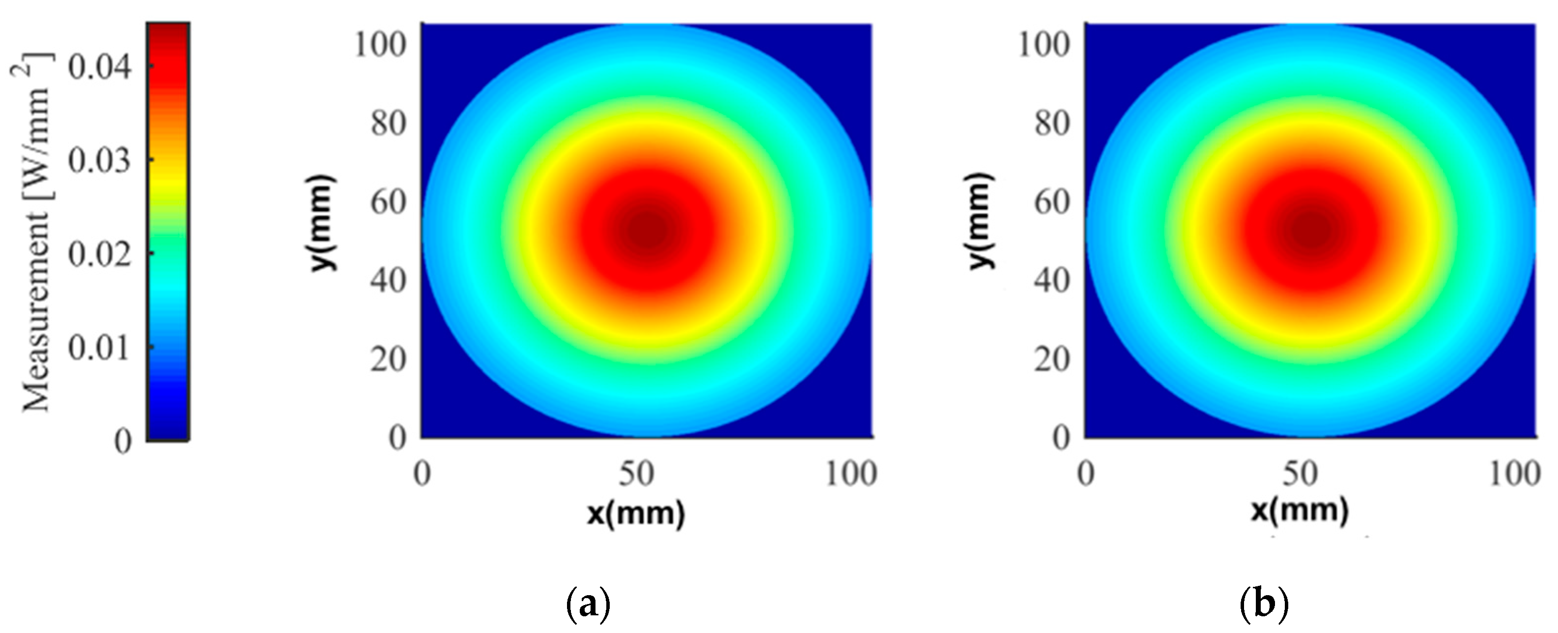
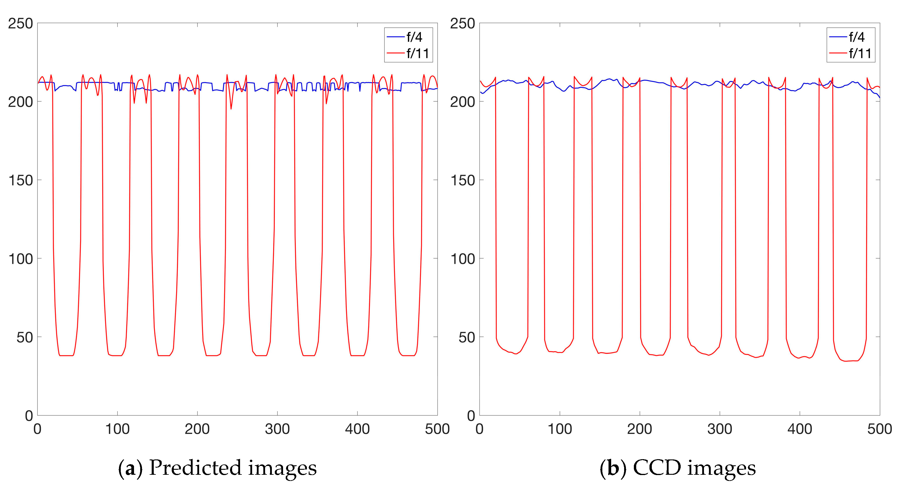
3.1. Validation through Analytic Solution

We designed and performed a digital phantom experiment to test the validity and accuracy of the proposed algorithm. The light propagation in the direct illumination case (with no intermediary optical components), which has an analytical solution, is examined in this digital phantom experiment. The experiment setup is shown in Figure 4.
A thin round plate with radius  R c  was set perpendicular to the optical axis, with the center aligned on the optical axis, beyond the lens with radius  R lens  and focal length  f . The light intensity was set to be uniform on the plate, given as  ψ . The distance from the aperture to the plate and the image plane was denoted by  l 1  and  l 2 ,  respectively. Furthermore, the focal length  f  and two distances  l 1  and  l 2  are set to follow the equation  1 f = 1 l 1 + 1 l 2  in the testing system. Furthermore, according to the Cosine fourth Power Law [38], the analytical solution  M e  for the received power per area on the image plane under these settings can be written as:
M e x ,   y = π ψ R lens 2 l 1 2 l 2 2 l 1 2 + R lens 2 ( l 2 2 + x 2 + y 2 ) , x 2 + y 2     R c 2 l 2 2 l 1 2 0 , x 2 + y 2   >   R c 2 l 2 2 l 1 2
In the numerical validation,  ψ  was set as  1   W / mm 2 / sr l 1 l 2  and  f  were set as 1050 mm, 52.5 mm, and 50 mm, respectively;  R lens  and  R c  were set as 6.25 mm and 1050 mm, respectively.
For validation purposes, the size of the numerical CCD chip is set to 105 mm × 105 mm. The CCD chip is discretized by 501 × 501 pixels. The predicted measurement  M c  is computed on every pixel with the light propagation model. The aperture is discretized with  N ρ = 10  and  N ω = 10 . The comparison between  M e  and  M c  is shown in Figure 4. No noticeable differences between the analytical measurement  M e  (Figure 5a) and the predicted measurement  M c  (Figure 5b) were observed. The relative error of  M c  is in the range  [ 0 ,   5 × 10 5 ) . To further quantify the performance of the back ray-tracing algorithm, the correlation factor  c M e , M c  and deviation factor  d M e , M c  of the computed measurement are computed as  c M e , M c = 1   1 . 4564   ×   10 10  and  d M e , M c = 3 . 5114   ×   10 5 , with the definitions of  c M e , M c  and  d M e , M c  given as:
c M c ,   M e : = i = 1 N M i c     M c ¯ M i e     M e ¯ N σ M c σ M e d M c ,   M e : = i = 1 N M i c     M i e 2 / N σ M e
where  N  is the number of voxels,  M -  and  σ M  are the weighted average and standard deviation. Therefore, the high correlation factor and low deviation factor, and relative error indicate that the free space light propagation model has very high accuracy for this case.

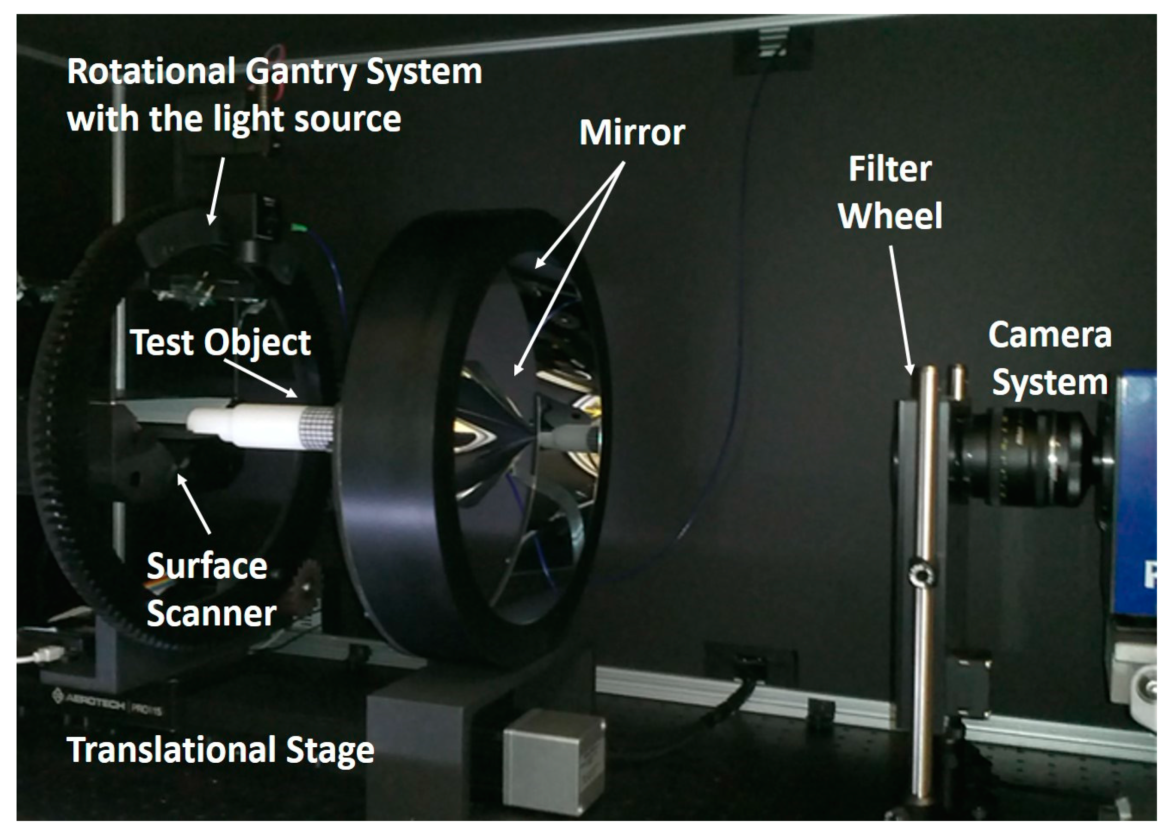
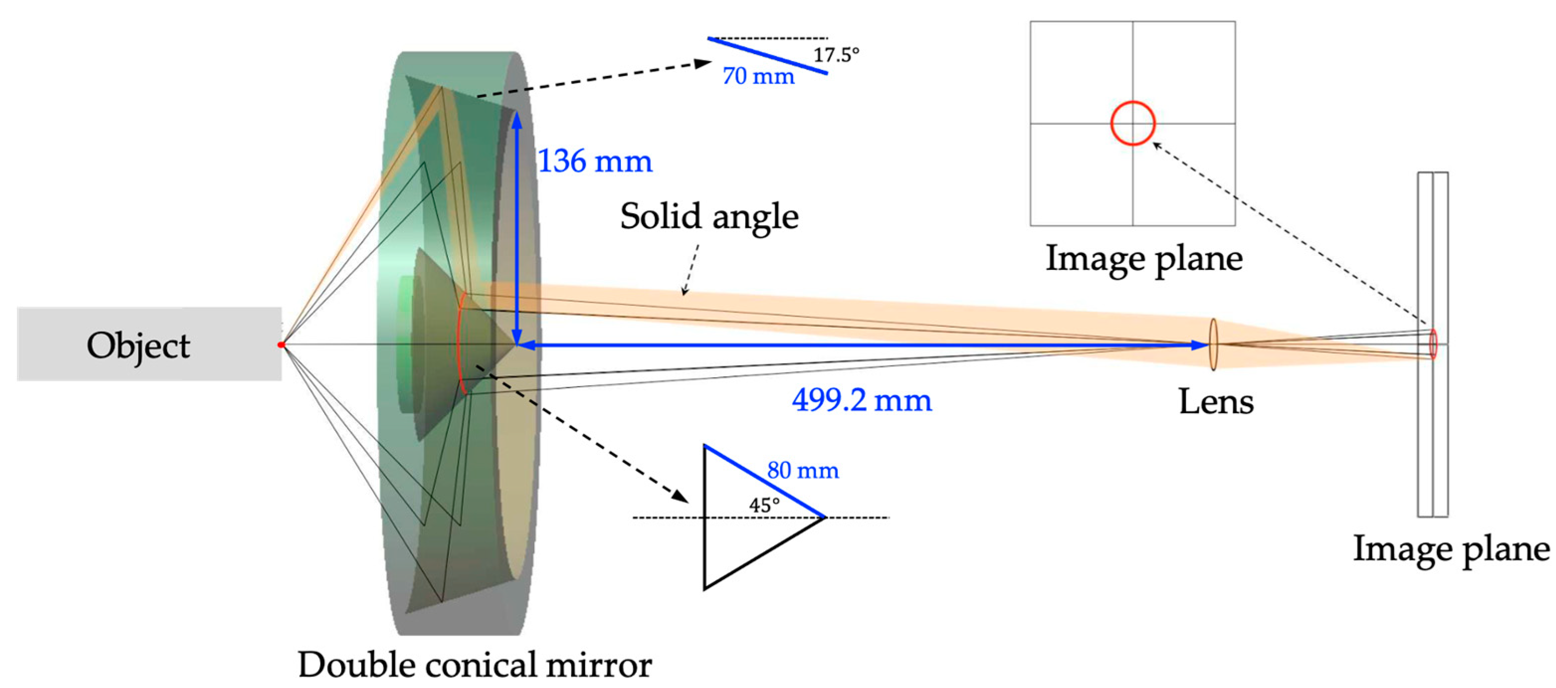
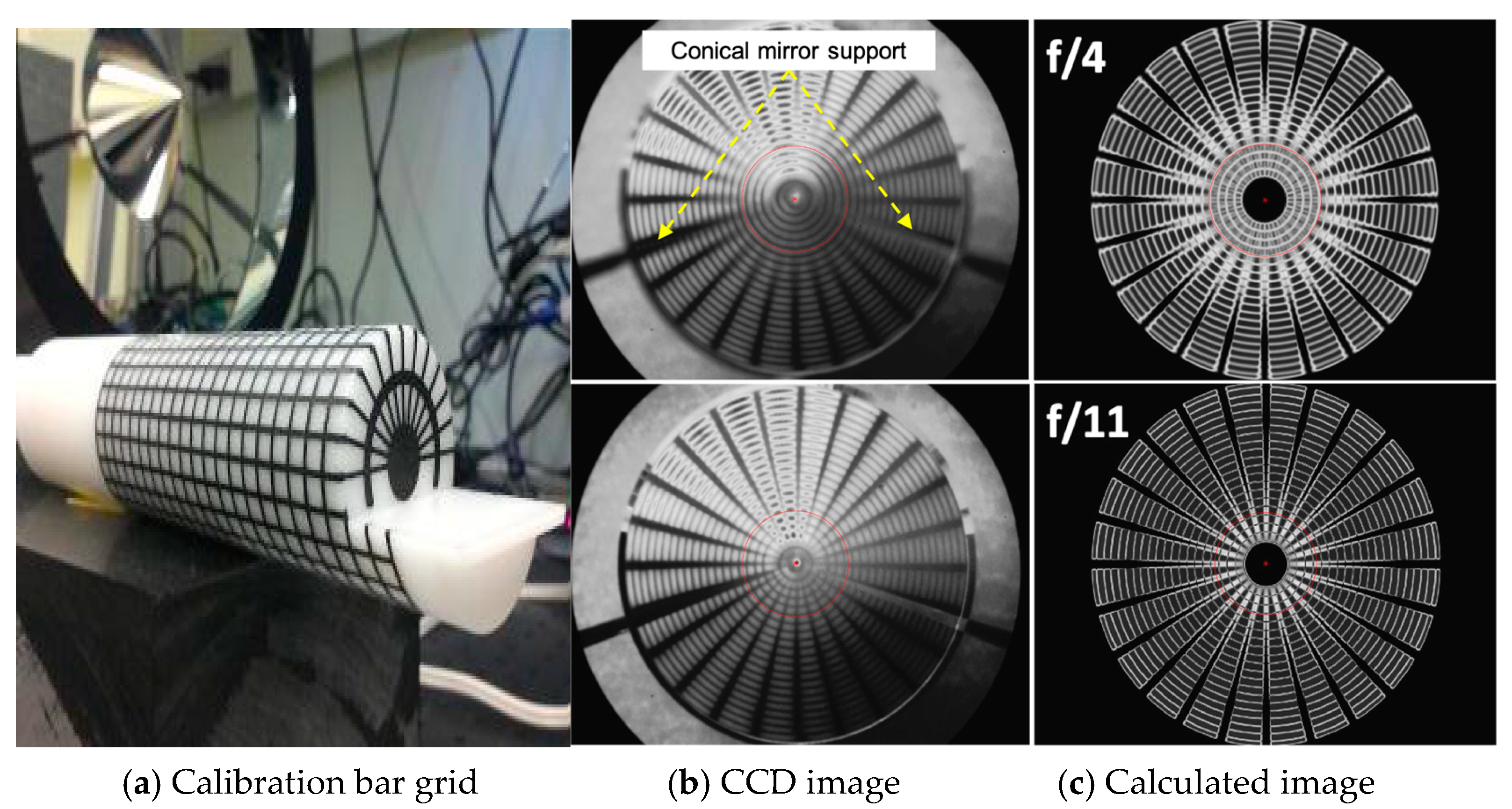
3.2. Validation through the Double Conical Mirror Non-Contact Imaging System

A double conical mirror system has been designed to capture multi-directional views simultaneously in small animal imaging [39] (See Figure 6). A. The first mirror facing a target captures a surface of the target, and the second mirror facing a detection camera reflects and projects the captured images by the first mirror onto the detection camera. Depending on the shape of a target, the shapes of the first and second mirrors can vary, like flat, conical, oval, or two combined shapes. For this system, since the target is a small animal, like mice, a conical shape is chosen to capture the whole-body surface of a small animal. The conical mirror size was designed to cover a 40 mm diameter, 80 mm length cylinder, the size of which is enough to cover a small animal.
This conical-mirror system provides the capability to obtain measurements of angular-resolved-data. Figure 7 provides a conceptual illustration through ray tracing of how the angle-resolved data can be obtained with the conical mirror. Consider, for example, a single point on the cylindrical target object positioned on the concentric axis of two conical mirrors inside the camera’s field of view. The conical mirrors distribute the viewing angle of the camera to the entire  360 o  around a single point. As a result, the camera image generated using ray tracing is not a point but a ring. Therefore, within the angular coverage of the conical mirror pairs, angular-resolved data can be obtained. Consequently, the measurement using the conical mirror imaging head can lead to a substantial improvement in the image reconstruction results.
We further tested the performance of our algorithm on this double conical mirror imaging system. To this end, we used a calibration bar grid as a target for imaging. Figure 8a shows the positioning of a calibration bar as a target in the imaging unit. The CCD images were taken by a camera through the double conical mirror system (Figure 8b). Figure 8c shows the images generated through the measurement operator that was constructed under the same settings as the actual conical mirror system by using our ray tracing algorithm as proposed in the previous section. Two experiments were conducted with two different values of f-number: f/4 and f/11. As shown in Figure 8, there is image distortion because of the conical shape of the mirrors.
As expected, sharper images were obtained with f/11 than with f/4. In other words, the black and white grid pattern of the calibration bar is clearly visible in both CCD and predicted images with f/11 used, whereas, for the f/4 case, the reduced depth of field is observed here that leads to a blurred or distorted image, i.e., the grid pattern in the foreground area is severely distorted to look like a ring. For quantitative comparison, a circle (red solid line) was placed over the images, as shown in Figure 8, and the pixel values were extracted along the circle except for the conical mirror support area for each image. The pixel values are then rescaled to fall within the same number scale, which mitigates the effect of the image scale difference between CCD and predicted images. Figure 9 shows the line profiles from CCD and predicted images obtained with f/4 and f/11, respectively. As shown in Figure 9, the grid pattern, which is represented by the high and low pixel values in the line profile, is well preserved with f/11 in both CCD and predicted images, while such a high-contrast grid pattern was almost lost by blurring in both images when f/4 was used. These results suggest the CCD images through the conical mirror system can be reasonably predicted by our ray tracing algorithm shown in the images. The correlation coefficient and deviation factor were also computed to be  c M CCD ,   M Pred = 0 . 82  and  d M CCD ,   M Pred = 0 . 64 . The large deviation factor is believed to be mainly because of the mismatch between the illumination conditions used for the experiment and the model. In fact, the CCD image was taken under ambient light conditions, while the ray tracing algorithm assumed a uniform light distribution on the calibration bar surface, although this may not be true. Discrepancies between measurements and predictions can be minimized once illumination conditions and system parameters are more accurately known for the experiment considered.

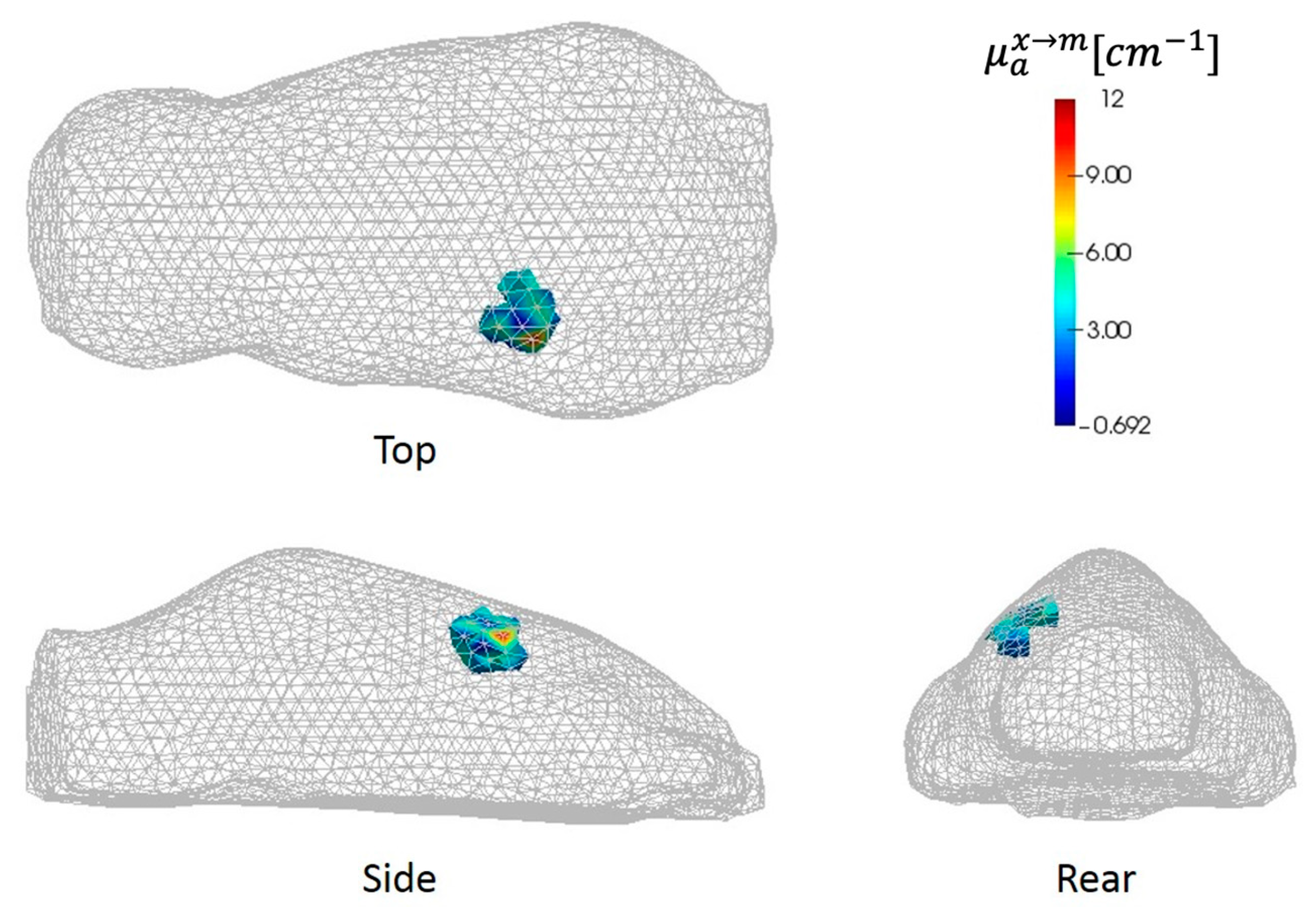
3.3. Application to Real Fluorescence Molecular Tomographic Imaging

A small animal fluorescence imaging experiment was conducted with a tumor-bearing mouse using the double conical mirror imaging system. Osteosarcoma cells (143B), transfected with GFP (pEGF-C1), were sorted to present 80-ek after to mea90% GFP positive expression. Considering the weak signals of GFP, the tumor cells (1 × 10⁶ cells/mL in 100 μL PBS) were injected subcutaneously near the left kidney of a mouse. Furthermore, the mouse was imaged one week later to measure the tumor growth through fluorescence molecular tomography (FMT). The excitation was done with a 475 nm wavelength, and the emission signal due to GFP-tagged tumor cells was measured with a 515 nm long-pass filter. The optical properties are  μ a = 0 . 4   cm 1    and  μ s = 15   cm 1    for absorption and scattering coefficients, respectively,  τ = 4.0   ns  for lifetime, and  η = 0.95  for quantum yield.
With one single illumination on the tumor area, 37,558 data points were obtained on the CCD image as measurements and used as input to the reconstruction code. The reconstructed map of the absorption coefficient  μ a x m  of a fluorescent source inside the mouse clearly shows the tumor location in Figure 10, which was confirmed by the planar imaging results using the Kodak In-vivo Multispectral Imaging System FX (Carestream Health, Inc., Rochester, NY, USA). It should be noted that this result is obtained with one single illumination alone.
Moreover, several published works have already applied the proposed model for measurement operator derivation and improved DOT results [39,40,41,42]. These results support the validity of the back ray-tracing model for light propagation in free space.

4. Conclusions

This work developed a novel free-space, angular-dependent photon transport model for deriving the measurement operator in a non-contact DOT imaging system. This model employed the backward ray-tracing method to efficiently calculate the surface radiation contribution to each pixel on the CCD chip by fully considering the angularly dependency of the light intensity.
The presented algorithm was validated by using both numerical experiments and actual measurement data. In the numerical experiment, the performance of the proposed algorithm was compared against an analytic solution and evaluated in terms of correlation factor, deviation factor, and relative error. It was shown from the results that the correlation factor was very close to 1 and the deviation factor was very close to 0, which indicates a solid agreement between the output of the proposed model and the analytical solution. Furthermore, the proposed algorithm has also been successfully applied to provide the measurement operator that allows the angle-resolved fluorescence data to be used for 3D tomographic results.
The results demonstrate that the proposed method based on backward-distributed ray tracing provides accurate modeling of the angle-dependent ray transfer function, which is crucial to non-contact camera-based DOT reconstructions with catadioptric systems that involve conical mirrors.
The backward ray tracing method presented here employed a discretization of the aperture alone. Therefore, the method can be further improved for more accurate prediction of CCD pixel measurements. This can be done by using a discretization of each CCD pixel in addition to the discretized aperture, which will be considered in future work.

Author Contributions

Conceptualization, methodology, software, data analysis, and visualization; S.H.K. and J.J.; writing—original draft preparation, S.H.K. and J.J.; writing—review and editing, S.H.K. and A.H.H.; resources, supervision, project administration, and funding acquisition, A.H.H. All authors have read and agreed to the published version of the manuscript.

Funding

This research was funded in part by grants from the National Heart, Lung and Blood Institute (NHLBI 1R01HL115336-01) and the National Institute of Arthritis and Musculoskeletal and Skin Diseases (NIAMS 5R01AR050026-10) at the National Institutes of Health (NIH) and in part by the National Cancer Institute (NCI#5R33CA118666-05) at the National Institute of Health (NIH).

Institutional Review Board Statement

Not applicable because this work is the secondary analysis of existing and published data and thus does not require IRB review.

Informed Consent Statement

Not applicable.

Data Availability Statement

Not applicable.

Acknowledgments

The authors would like to thank Jonghwan Lee for his insightful comments and suggestions on the conical imaging system.

Conflicts of Interest

The authors declare no conflict of interest.

References

  1. Altoe, M.L.; Kalinsky, K.; Marone, A.; Kim, H.K.; Guo, H.; Hibshoosh, H.; Tejada, M.; Crew, K.; Accordino, M.; Trivedi, M.; et al. Changes in diffuse-optical-tomography images during early stages of neoadjuvant chemotherapy correlate with tumor response in different breast cancer subtypes. Clin. Cancer Res. 2021, 27, 1949–1957. [Google Scholar] [CrossRef] [PubMed]
  2. Gunther, J.E.; Lim, E.A.; Kim, H.K.; Flexman, M.; Altoé, M.; Campbell, J.A.; Hibshoosh, H.; Crew, K.D.; Kalinsky, K.; Hershman, D.; et al. Dynamic Diffuse Optical Tomography for Monitoring Neoadjuvant Chemotherapy in Patients with Breast Cancer. Radiology 2018, 287, 778–786. [Google Scholar] [CrossRef] [PubMed] [Green Version]
  3. Tromberg, B.J.; Pogue, B.W.; Paulsen, K.D.; Yodh, A.G.; Boas, D.A.; Cerussi, A.E. Assessing the future of diffuse optical imaging technologies for breast cancer management. Med. Phys. 2008, 35, 2443–2451. [Google Scholar] [CrossRef] [PubMed] [Green Version]
  4. Kim, S.H.; Montejo, L.; Hielscher, A.H. Diagnostic Evaluation of Rheumatoid Arthritis(RA) in Finger Joints Based on the Third-Order Simplified Spherical Harmonics (SP3) Light Propagation Model. Appl. Sci. 2022, 12, 6418. [Google Scholar] [CrossRef]
  5. Hielscher, A.H.; Kim, H.K.; Montejo, L.D.; Blaschke, S.; Netz, U.J.; Zwaka, P.A.; Illing, G.; Muller, G.A.; Beuthan, J. Frequency-Domain Optical Tomographic Imaging of Arthritic Finger Joints. IEEE Trans. Med. Imaging 2011, 30, 1725–1736. [Google Scholar] [CrossRef] [PubMed]
  6. Hielscher, A.H.; Klose, A.D.; Scheel, A.K.; Moa-Anderson, B.; Backhaus, M.; Netz, U.; Beuthan, J. Sagittal laser optical tomography for imaging of rheumatoid finger joints. Phys. Med. Biol. 2004, 49, 1147–1163. [Google Scholar] [CrossRef] [PubMed] [Green Version]
  7. Wang, Q.; Liu, Z.; Jiang, H. Optimization and evaluation of a three-dimensional diffuse optical tomography system for brain imaging. J. X-ray Sci. Technol. 2007, 15, 223–234. [Google Scholar]
  8. Fishell, A.K.; Burns-Yocum, T.M.; Bergonzi, K.M.; Eggebrecht, A.T.; Culver, J.P. Mapping brain function during naturalistic viewing using high-density diffuse optical tomography. Sci. Rep. 2019, 9, 11115. [Google Scholar] [CrossRef] [Green Version]
  9. Marone, A.; Hoi, J.W.; Khalil, M.A.; Kim, H.K.; Shrikhande, G.; Dayal, R.; Bajakian, D.R.; Hielscher, A.H. Modeling of the hemodynamics in the feet of patients with peripheral artery disease. Biomed. Opt. Express 2019, 10, 657–669. [Google Scholar] [CrossRef]
  10. Khalil, M.A.; Kim, H.K.; Kim, I.-K.; Flexman, M.; Dayal, R.; Shrikhande, G.; Hielscher, A.H. Dynamic diffuse optical tomography imaging of peripheral arterial disease. Biomed. Opt. Express 2012, 3, 2288–2298. [Google Scholar] [CrossRef] [Green Version]
  11. Zhang, X.F.; Badea, C. Effects of sampling strategy on image quality in noncontact panoramic fluorescence diffuse optical tomography for small animal imaging. Opt. Express 2009, 17, 5125–5138. [Google Scholar] [CrossRef]
  12. Da Silva, A.; Dinten, J.-M.; Coll, J.-L.; Rizo, P. From bench-top small animal diffuse optical tomography towards clinical imaging. In Proceedings of the 29th Annual International Conference of the IEEE Engineering in Medicine and Biology Society, Lyon, France, 2–26 August 2007; Volume 1–16, pp. 526–529. [Google Scholar]
  13. Chaudhari, A.J.; Darvas, F.; Bading, J.R.; Moats, R.A.; Conti, P.S.; Smith, D.J.; Cherry, S.R.; Leahy, R.M. Hyperspectral and multispectral bioluminescence optical tomography for small animal imaging. Phys. Med. Biol. 2005, 50, 5421–5441. [Google Scholar] [CrossRef]
  14. Arridge, S.R.; Dorn, O.; Kaipio, J.P.; Kolehmainen, V.; Schweiger, M.; Tarvainen, T.; Vauhkonen, M.; Zacharopoulos, A. Reconstruction of subdomain boundaries of piecewise constant coefficients of the radiative transfer equation from optical tomography data. Inverse Probl. 2006, 22, 2175–2196. [Google Scholar] [CrossRef]
  15. Kim, H.K.; Zhao, Y.; Raghuram, A.; Robinson, J.T.; Veeraraghavan, A.N.; Hielscher, A.H. Ultrafast and Ultrahigh-Resolution Diffuse Optical Tomography for Brain Imaging with Sensitivity Equation based Noniterative Sparse Optical Reconstruction (SENSOR). J. Quant. Spectrosc. Radiat. Transf. 2021, 276, 107939. [Google Scholar] [CrossRef]
  16. Kim, H.K.; Hielscher, A.H. A PDE-constrained SQP algorithm for optical tomography based on the frequency-domain equation of radiative transfer. Inverse Probl. 2009, 25, 015010. [Google Scholar] [CrossRef] [Green Version]
  17. Eda, H.; Oda, I.; Ito, Y.; Wada, Y.; Oikawa, Y.; Tsunazawa, Y.; Takada, M.; Tsuchiya, Y.; Yamashita, Y.; Oda, M.; et al. Multichannel time-resolved optical tomographic imaging system. Rev. Sci. Instrum. 1999, 70, 3595–3602. [Google Scholar] [CrossRef]
  18. Solomon, M.; White, B.R.; Nothdruft, R.E.; Akers, W.; Sudlow, G.; Eggebrecht, A.T.; Achilefu, S.; Culver, J.P. Video-rate fluorescence diffuse optical tomography for in vivo sentinel lymph node imaging. Biomed. Opt. Express 2011, 2, 3267–3277. [Google Scholar] [CrossRef] [PubMed] [Green Version]
  19. Mehta, A.D.; Jung, J.C.; Flusberg, B.A.; Schnitzer, M.J. Fiber optic in vivo imaging in the mammalian nervous system. Curr. Opin. Neurobiol. 2004, 14, 617–628. [Google Scholar] [CrossRef] [Green Version]
  20. Ripoll, J.; Schulz, R.B.; Ntziachristos, V. Free-space propagation of diffuse light: Theory and experiments. Phys. Rev. Lett. 2003, 91, 103901. [Google Scholar] [CrossRef]
  21. Schulz, R.B.; Ripoll, J.; Ntziachristos, V. Noncontact optical tomography of turbid media. Opt. Lett. 2003, 28, 1701–1703. [Google Scholar] [CrossRef] [PubMed]
  22. Meyer, H.; Garofaiakis, A.; Zacharakis, G.; Psycharakis, S.; Mamalaki, C.; Kioussis, D.; Economou, E.N.; Ntziachristos, V.; Ripoll, J. Noncontact optical imaging in mice with full angular coverage and automatic surface extraction. Appl. Opt. 2007, 46, 3617–3627. [Google Scholar] [CrossRef] [Green Version]
  23. Schulz, R.B.; Peter, J.; Semmler, W.; D’Andrea, C.; Valentini, G.; Cubeddu, R. Comparison of noncontact and fiber-based fluorescence-mediated tomography. Opt. Lett. 2006, 31, 769–771. [Google Scholar] [CrossRef]
  24. Elaloufi, R.; Arridge, S.; Pierrat, R.; Carminati, R. Light propagation in multilayered scattering media beyond the diffusive regime. Appl. Opt. 2007, 46, 2528–2539. [Google Scholar] [CrossRef]
  25. Dehghani, H.; Brooksby, B.; Vishwanath, K.; Pogue, B.W.; Paulsen, K.D. The effects of internal refractive index variation in near-infrared optical tomography: A finite element modelling approach. Phys. Med. Biol. 2003, 48, 2713–2727. [Google Scholar] [CrossRef] [PubMed]
  26. Wang, L.H.; Jacques, S.L.; Zheng, L.Q. MCML—Monte-Carlo Modeling of Light Transport in Multilayered Tissues. Comput. Methods Programs Biomed. 1995, 47, 131–146. [Google Scholar] [CrossRef] [PubMed]
  27. Atif, M.; Khan, A.; Ikram, M. Modeling of Light Propagation in Turbid Medium Using Monte Carlo Simulation Technique. Opt. Spectrosc. 2011, 111, 107–112. [Google Scholar] [CrossRef]
  28. Kumari, S.; Nirala, A.K. Study of light propagation in human and animal tissues by Monte Carlo simulation. Indian J. Phys. 2012, 86, 97–100. [Google Scholar] [CrossRef]
  29. Chen, X.L.; Gao, X.B.; Qu, X.C.; Chen, D.F.; Ma, X.P.; Liang, J.M.; Tian, J. Generalized free-space diffuse photon transport model based on the influence analysis of a camera lens diaphragm. Appl. Opt. 2010, 49, 5654–5664. [Google Scholar] [CrossRef]
  30. Chen, X.L.; Gao, X.B.; Qu, X.C.; Liang, J.M.; Wang, L.; Yang, D.A.; Garofalakis, A.; Ripoll, J.; Tian, J. A study of photon propagation in free-space based on hybrid radiosity-radiance theorem. Opt. Express 2009, 17, 16266–16280. [Google Scholar] [CrossRef] [Green Version]
  31. Duma, V.-F. Radiometric versus geometric, linear, and nonlinear vignetting coefficient. Appl. Opt. 2009, 48, 6355–6364. [Google Scholar] [CrossRef]
  32. Strojnik, M.; Bravo-Medina, B.; Martin, R.; Wang, Y. Ensquared Energy and Optical Centroid Efficiency in Optical Sensors: Part 1, Theory. Photonics 2023, 10, 254. [Google Scholar] [CrossRef]
  33. Gao, H.; Zhao, H. Multilevel bioluminescence tomography based on radiative transfer equation Part1: L1 regularization. Opt. Express 2010, 18, 1854–1871. [Google Scholar] [CrossRef] [PubMed]
  34. Modest, M.F. Radiative Heat Transfer, 2nd ed.; Academic Press: Cambridge, MA, USA, 2003. [Google Scholar]
  35. Meseguer, J.; Perez-Grande, I.; Sanz-Andres, A. Thermal Radiation Heat Transfer; Woodhead Publ. Mech.: Cambridge, UK, 2012; Volume E, pp. 73–86. [Google Scholar]
  36. Coxeter, H.S.M. Barycentric Coordinates, 2nd ed.; §13.7 in Introduction to Geometry; Wiley: New York, NY, USA, 1969; pp. 216–221. [Google Scholar]
  37. Holmes, M.H. Introduction to Perturbation Methods, 2nd ed.; Springer: New York, NY, USA, 2013. [Google Scholar]
  38. Cook, R.L.; Porter, T.; Carpenter, L. Distributed Ray Tracing. In Proceedings of the 11th Annual Conference on Computer Graphics and Interactive Techniques, Minneapolis, MN, USA, 23–27 July 1984; Volume 18, pp. 137–145. [Google Scholar]
  39. Gardner, I.C. Validity of the Cosine 4th Power Law of Illumination. J. Res. Nat. Bur. Stand. 1947, 39, 213–219. [Google Scholar] [CrossRef]
  40. Lee, J.H.; Kim, H.K.; Chandhanayingyong, C.; Lee, F.Y.I.; Hielscher, A.H. Non-contact small animal fluorescence imaging system for simultaneous multi-directional angular-dependent data acquisition. Biomed. Opt. Express 2014, 5, 2301–2316. [Google Scholar] [CrossRef] [Green Version]
  41. Lee, J.H.; Kim, H.K.; Jia, J.; Fong, C.; Hielscher, A.H. A Fast full-body fluorescence/bioluminescence imaging system for small animals. Opt. Tomogr. Spectrosc. Tissue X 2013, 8578, 857821. [Google Scholar]
  42. Hoi, J.W.; Kim, H.K.; Fong, C.J.; Zweck, L.; Hielscher, A.H. Non-contact dynamic diffuse optical tomography imaging system for evaluating lower extremity vasculature. Biomed. Opt. Express 2018, 9, 5597–5614. [Google Scholar] [CrossRef]
Figure 1. Surface radiation and emissive power.
Photonics 10 00767 g001
Figure 2. An illustration of (a) surface discretization with triangle elements and (b) a triangle element  Γ  and a location vector  r .
Photonics 10 00767 g002
Figure 3. An illustration of a simplified model of the CCD camera.
Photonics 10 00767 g003
Figure 4. Light propagation from the object’s surface, through the optical system, to the image plane of the CCD camera.
Photonics 10 00767 g004
Figure 5. Comparison between the exact and the computed measurement on the image plane; (a) The exact measurement; (b) The measurements computed with the back ray-tracing model.
Photonics 10 00767 g005
Figure 6. A picture of the double conical mirror system.
Photonics 10 00767 g006
Figure 7. Angular-resolved measurements using the conical mirror pair. The captured image of a single point in the conical mirror pair scheme is a ring.
Photonics 10 00767 g007
Figure 8. A picture of the calibration bar with the double conical mirror system. (a) Calibration bar in the imaging unit; (b) the captured image on the camera; (c) the calculated image using the ray tracing algorithm with (21). Note that a red circle on the image represents a region of interest for quantitative analysis.
Photonics 10 00767 g008
Figure 9. The line profiles extracted with f/4 and f/11 along the circle: (a) predicted images; (b) CCD images.
Photonics 10 00767 g009
Figure 10. Reconstruction results of the tumor growth one week after subcutaneous tumor injection.
Photonics 10 00767 g010
Disclaimer/Publisher’s Note: The statements, opinions and data contained in all publications are solely those of the individual author(s) and contributor(s) and not of MDPI and/or the editor(s). MDPI and/or the editor(s) disclaim responsibility for any injury to people or property resulting from any ideas, methods, instructions or products referred to in the content.

