Communication

High-Precision Laser Self-Mixing Displacement Sensor Based on Orthogonal Signal Phase Multiplication Technique

1
Department of Physics, Jimei University, Xiamen 361021, China
2
Department of Electronics Engineering, Xiamen University, Xiamen 361005, China
*
Author to whom correspondence should be addressed.
Photonics 2023, 10(5), 575; https://doi.org/10.3390/photonics10050575
Submission received: 8 March 2023 / Revised: 28 April 2023 / Accepted: 9 May 2023 / Published: 14 May 2023

Abstract

:
A new signal processing method named orthogonal signal phase multiplication (OSPM) is proposed, which is used to improve the precision of vibration measurement in a phase-modulating self-mixing interferometer (SMI). The modulated signal is acquired by an electro-optic modulator, which is placed in the external cavity. Higher measurement precision is realized by performing the phase multiplication algorithm on the orthogonal signals extracted from the harmonic components of the signal spectrum. Theoretically, the displacement reconstruction precision of OSPM is higher than that of conventional modulation methods, and it can be continuously improved by increasing the multiplication times. The feasibility and performance of the proposed method are verified by simulated signals and confirmed by experiments; the absolute error is less than 11 nm, and relative error is less than 0.75%, within the amplitude range from 661 nm to 2013 nm. This method does not involve additional optical elements, and its effectiveness meet the requirements for real-time high-precision measurements.

1. Introduction

With the development of advanced manufacturing, biomedicine, and many other leading-edge fields, the requirement for micro motion measurement at the nanometer level is increasing [1,2,3,4,5]. As a new interferometry technology, SMI has been widely used in the field of precision measurement. So-called self-mixing interference refers to the fact that a part of the reflected or scattered light feedbacks into the laser cavity and interferes with the original light, resulting in changes in laser output characteristics. Compared with traditional interferometry used to measure the motion of an external target, self-mixing interferometry has been applied in many sensing fields, such as distance [6,7,8,9], angle [10,11,12], displacement [13,14,15,16], velocity [17,18,19], and other fields [20,21,22,23], due to its inherent advantages, such as its simple and compact structure, self-alignment, and low cost.
Over the past 20 years, many measurement techniques based on the SMI technique have been proposed, the simplest of which is the fringe counting method [24], where each fringe corresponds to λ 0 / 2 of the displacement of the external target, where λ 0 is the laser wavelength without optical feedback. In order to improve the basic resolution of λ 0 / 2 , many algorithms based on the phase unwrapping method (PUM) have been proposed [25], with the accuracy of reconstruction ranging from λ 0 / 8 to λ 0 / 60. Although the PUM provides quite good precision for LD-based self-mixing systems, it is computationally complex and time consuming, because it needs iterative routines to estimate the optical feedback parameter and the linewidth enhancement factor α , which makes it inefficient in real-time, high-bandwidth, embedded sensing applications. Moreover, the accuracy and the effectiveness of this method will be affected by noise, the speckle effect, and other environmental factors. In order to reduce its sensitivity to the fluctuations of laser power and ambient noise, a variety of phase modulation methods have been proposed [26,27,28]. Although the proposed modulation methods, such as EOM (electro-optic modulator), have relatively high precision of reconstruction and strong anti-interference ability, it is difficult to further improve their accuracy. In recent years, there have been some algorithms that can reconstruct the displacement at less than λ 0 / 2 , but such algorithms still have some inherent problems. Ali et al., using spectral processing, achieved nanometric vibration sensing, but the algorithm is complicated and can only recover target vibrations with an amplitude larger than λ 0 / 8 [29]. Lu et al. proposed a method based on reflective phase modulation, which uses the high-frequency vibration mirror as the modulation device of the system; therefore, the reconstruction accuracy can be improved, and the ability to measure an amplitude less than λ 0 / 2 is achieved [30]. However, this method requires accurately adjusting the position of PZTs (piezoelectric transducers) in the optical path, which is hard to do in practical conditions and damages the inherent simplicity of the self-mixing system.
In this paper, an orthogonal signal phase multiplication algorithm is introduced into a phase-modulating SMI system for improving the measurement accuracy. Through the operation of harmonic components of the signal spectrum, the wrapped signal with doubled phase can be obtained, and the displacement of the vibrating target can be reconstructed with higher precision. Since the proposed method does not require additional optical devices or optical path adjustments, the entire system retains its inherent simplicity. In addition, it has the advantage of scalable accuracy, by setting the multiplication times, which gives it wide application prospects in the field of micro vibration measurement at the nanometer scale.

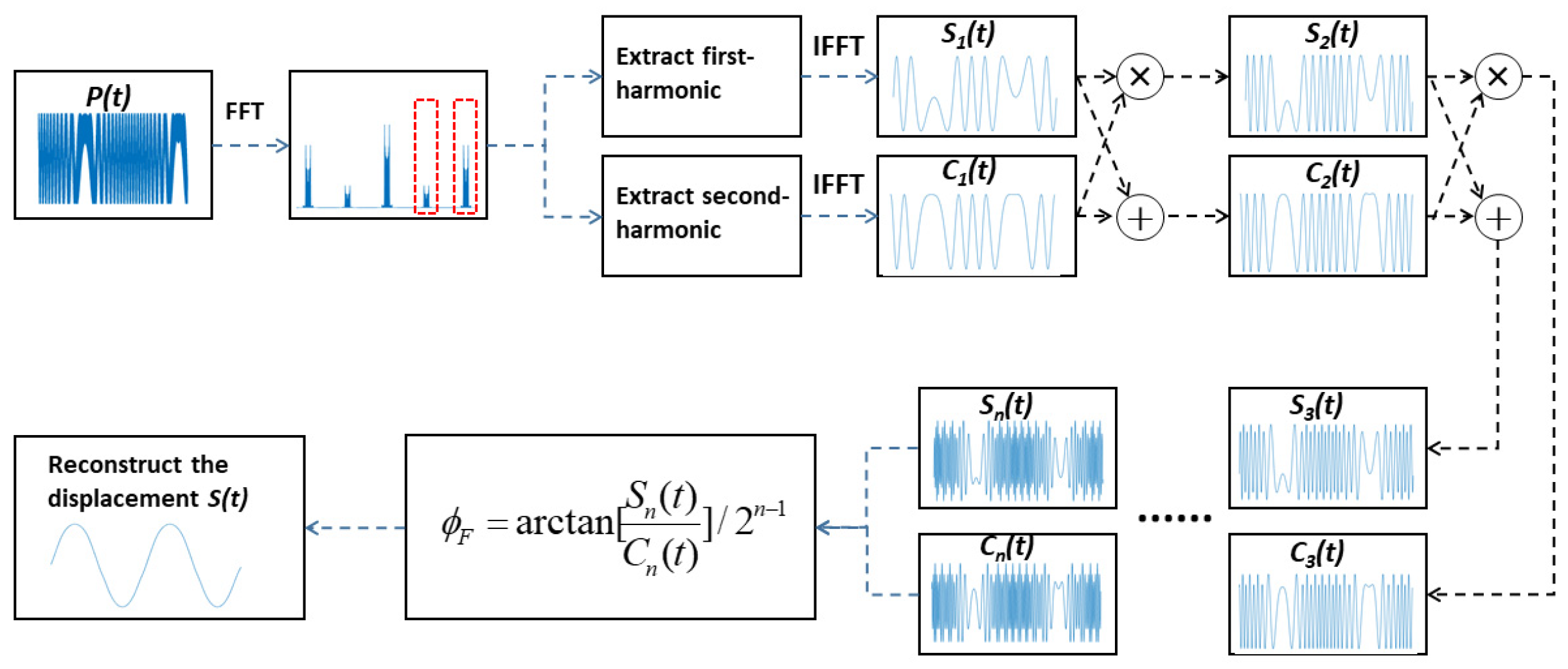
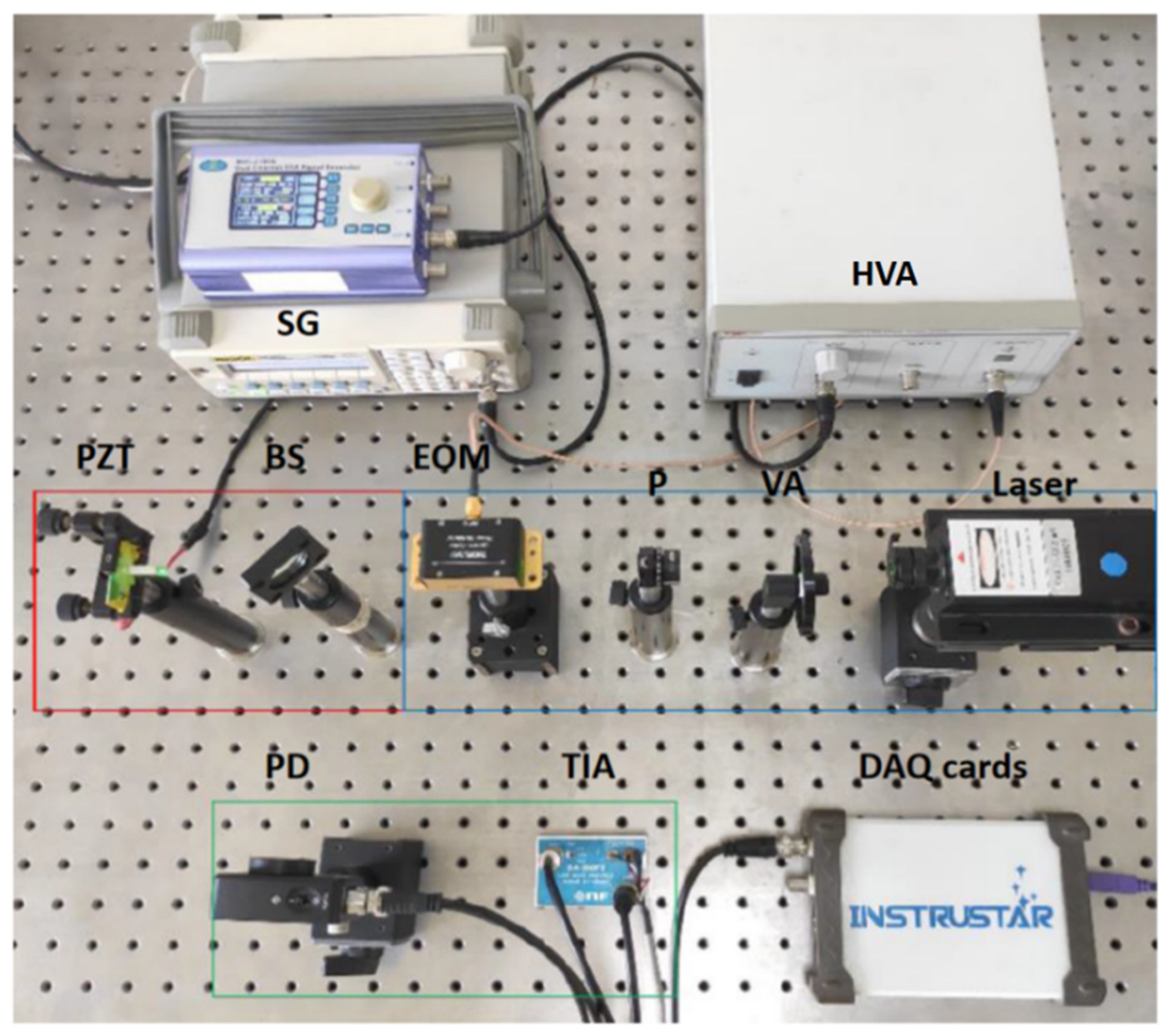
2. Measurement Principle

According to the three-facet Fabry–Perot model [31], when sinusoidal phase modulation is introduced into the SMI, the transmitted power P under a weak feedback regime can be expressed as:
P = P 0 { 1 + m c o s ϕ F + Ψ ( t ) }
Here, P0 is the power of the laser output without feedback; m is the modulation coefficient; ϕ F = 4 π L ( t ) / λ 0 is the measured phase of the external cavity; λ0 is the central wavelength of the laser; and Ψ ( t ) = 2 h s i n ( 2 π f w t + β ) is the sinusoidal phase modulation term. Considering that the light beam passes through the EOM twice in the external cavity, the sinusoidal phase modulation depth is 2 h . The frequency and initial phase are f w and β , respectively. Expanding Equation (1) with the Bessel function after DC (direct current) blocking and normalization processing, it can be expressed as [32]:
P = cos ( ϕ F ) J 0 ( 2 h ) + 2 cos ( ϕ F ) × n = 1 J 2 n ( 2 h ) cos [ ( 2 n ) ( 2 π f w t + β ) ] 2 sin ( ϕ F ) × n = 1 J 2 n 1 ( 2 h ) cos [ ( 2 n 1 ) ( 2 π f w t + β ) ]
Here, J n ( 2 h ) is the first type Bessel function of order n, and J 2 n ( 2 h ) and J 2 n 1 ( 2 h ) are the even and odd orders, respectively. It can be seen that the AC component of the SMI signal is composed of the fundamental frequency f w and its harmonics, and the odd harmonics fluctuate with sin ( ϕ F ) , while the even harmonics fluctuate with cos ( ϕ F ) .
According to the Equation (2), the first and second harmonic components can be expressed as follows:
P 1 ( t ) = 2 sin ( ϕ F ) J 1 ( 2 h ) cos ( 2 π f w t + β ) = A 1 ( t ) cos ( 2 π f w t + β )
P 2 ( t ) = 2 cos ( ϕ F ) J 2 ( 2 h ) cos ( 4 π f w t + 2 β ) = A 2 ( t ) cos ( 4 π f w t + 2 β )
Here, the A 1 ( t ) = 2 sin ( ϕ F ) J 1 ( 2 h ) and A 2 ( t ) = 2 cos ( ϕ F ) J 2 ( 2 h ) represent the strengths of the first and second harmonic components, respectively. As can be seen, A 1 ( t ) and A 2 ( t ) are composed by sine and cosine functions of the feedback phase of the system, respectively, and the values of first-order and second-order Bessel functions, respectively. Therefore, the orthogonal signals can be obtained by dividing the corresponding value of the Bessel functions. Then, the required phase ϕ F can be calculated. The specific calculation process is as follows:
sin ϕ F = A 1 ( t ) / 2 J 1 ( 2 h ) = S 1 ( t )
cos ϕ F = A 2 ( t ) / 2 J 2 ( 2 h ) = C 1 ( t )
Φ F = a r c t a n [ S 1 ( t ) C 1 ( t ) ]
Here, A 1 ( t ) and A 2 ( t ) can be obtained by eliminating the carrier of P 1 ( t ) and P 2 ( t ) , respectively. The specific formulas for eliminating the carrier are as follows:
A 1 ( t ) = I m [ P 1 ( t ) / e j ( 2 π f w + β ) ]
A 2 ( t ) = R e [ P 2 ( t ) / e j ( 4 π f w + β ) ]
Therefore, after normalizing the A 1 ( t ) and A 2 ( t ) , the S 1 ( t ) and C 1 ( t ) can be obtained.
The principle of phase multiplication can be illustrated as follows. First, based on the double angle formula combined with previous equations, we can obtain:
S 2 ( t ) = 2 S 1 ( t ) C 1 ( t ) = sin 2 ϕ F = sin 2 × 4 π L ( t ) λ
C 2 ( t ) = C 1 2 ( t ) S 1 2 ( t ) = cos 2 ϕ F = cos 2 × 4 π L ( t ) λ
From Equations (10) and (11), it can be clearly seen that the phase of the processed signal S 2 ( t ) and C 2 ( t ) has doubled after the operation, and this indicates that L ( t ) only needs to change λ 0 /4 to produce one fringe.
Similarly, S n ( t ) and C n ( t ) can be obtained by the same process. After that, ϕ F can be solved by:
ϕ F = a r c t a n S n ( t ) C n ( t ) / 2 n 1
According to the preceding analysis, the process of vibration measurement using orthogonal signal phase multiplication technique is shown in Figure 1. First, perform the fast Fourier transform (FFT) on the SMI signal to obtain the Fourier spectra; then, the frequency content is fed to two band-pass filters to extract the first and second harmonics. After inverse fast Fourier transform (IFFT), the orthogonal signals S 1 ( t ) and C 1 ( t ) are obtained, respectively. According to Equations (10) and (11), S 2 ( t ) and C 2 ( t ) are easily obtained by doing the phase multiplication operation. Similarly, S n ( t ) and C n ( t ) are obtained by the same process. Then, the curves S n ( t ) and C n ( t ) are used to determine the wrapped measured phase. Finally, a phase unwrapping process is employed to reconstruct a continuous phase variation of the SMI signal.

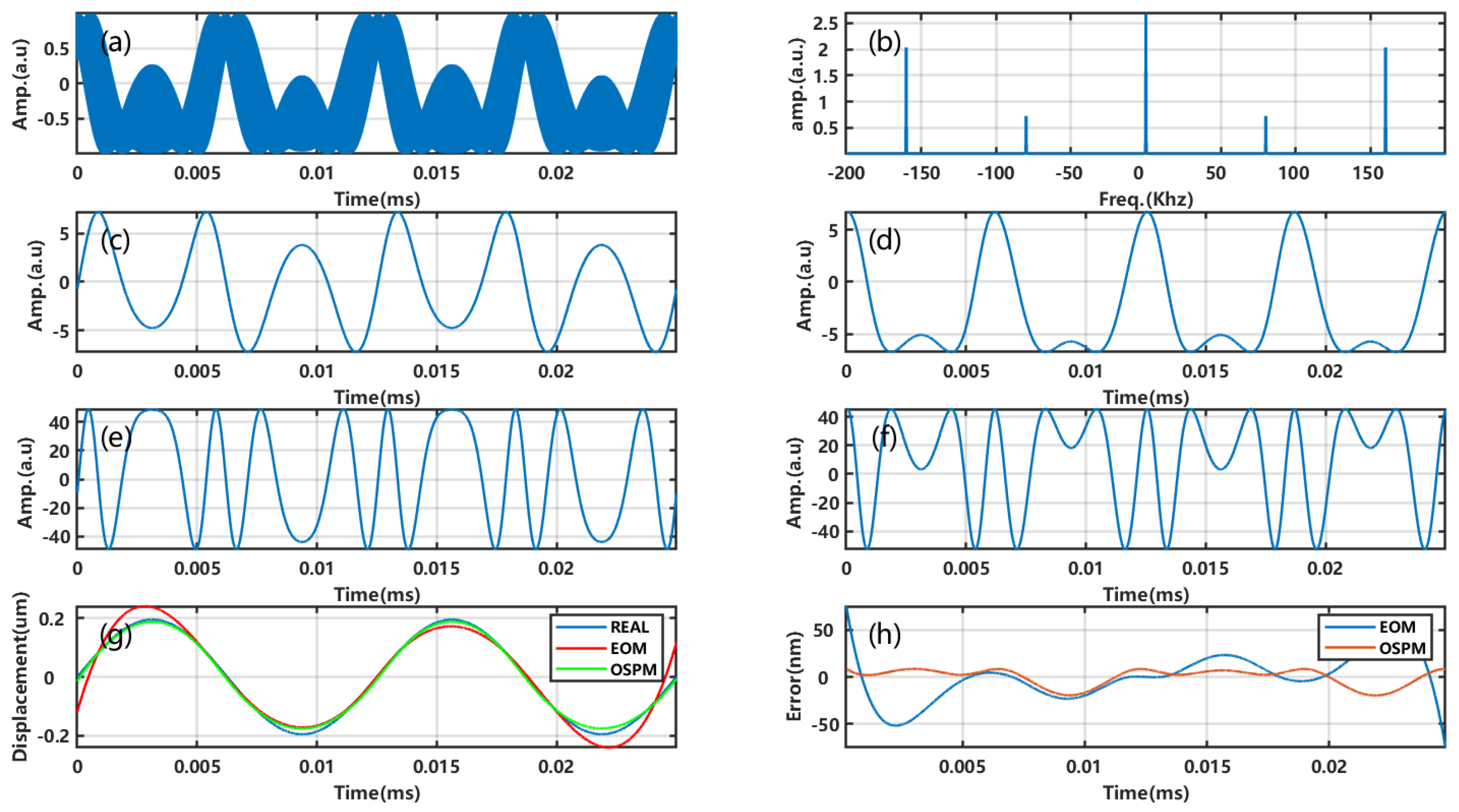
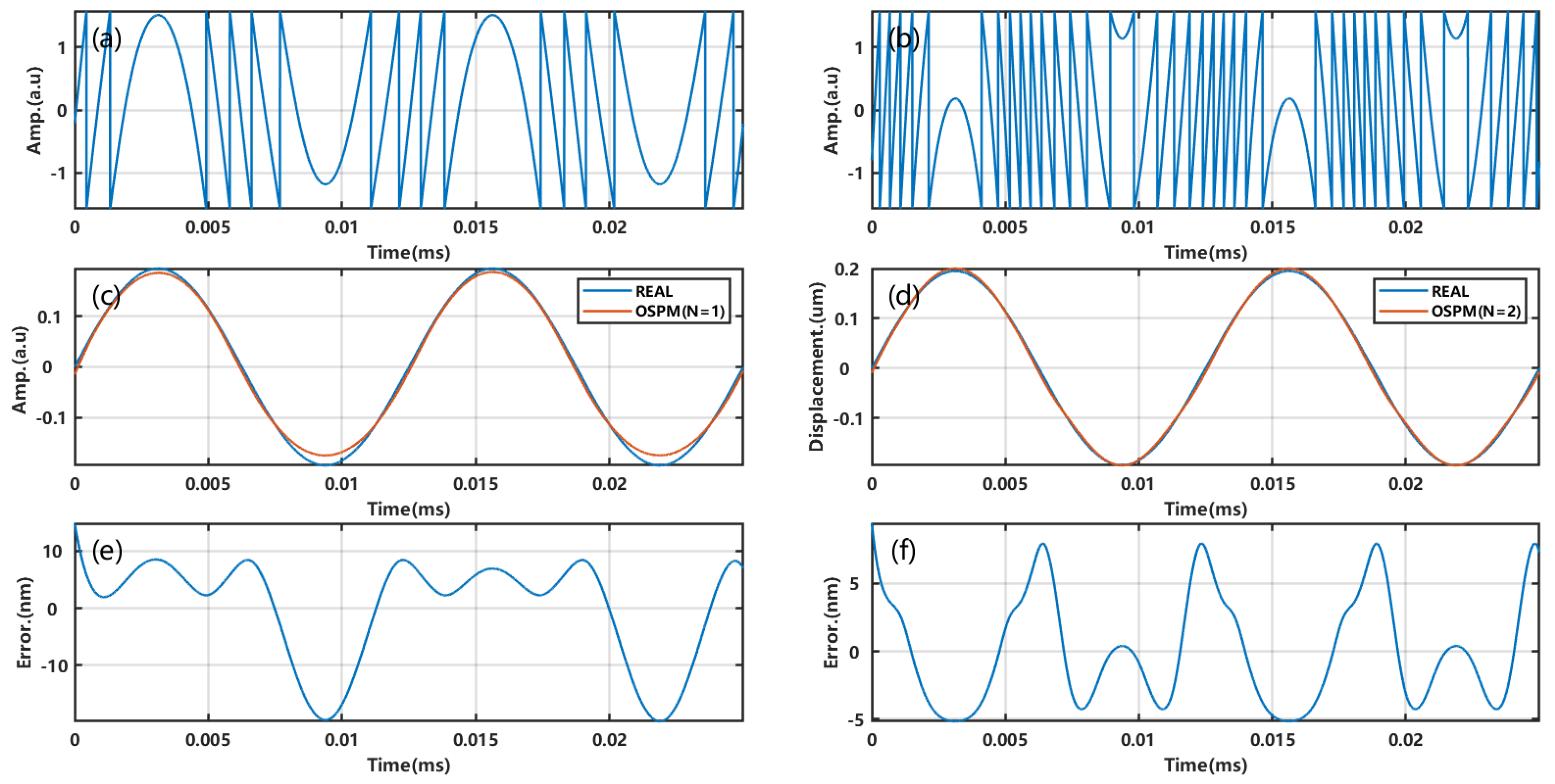
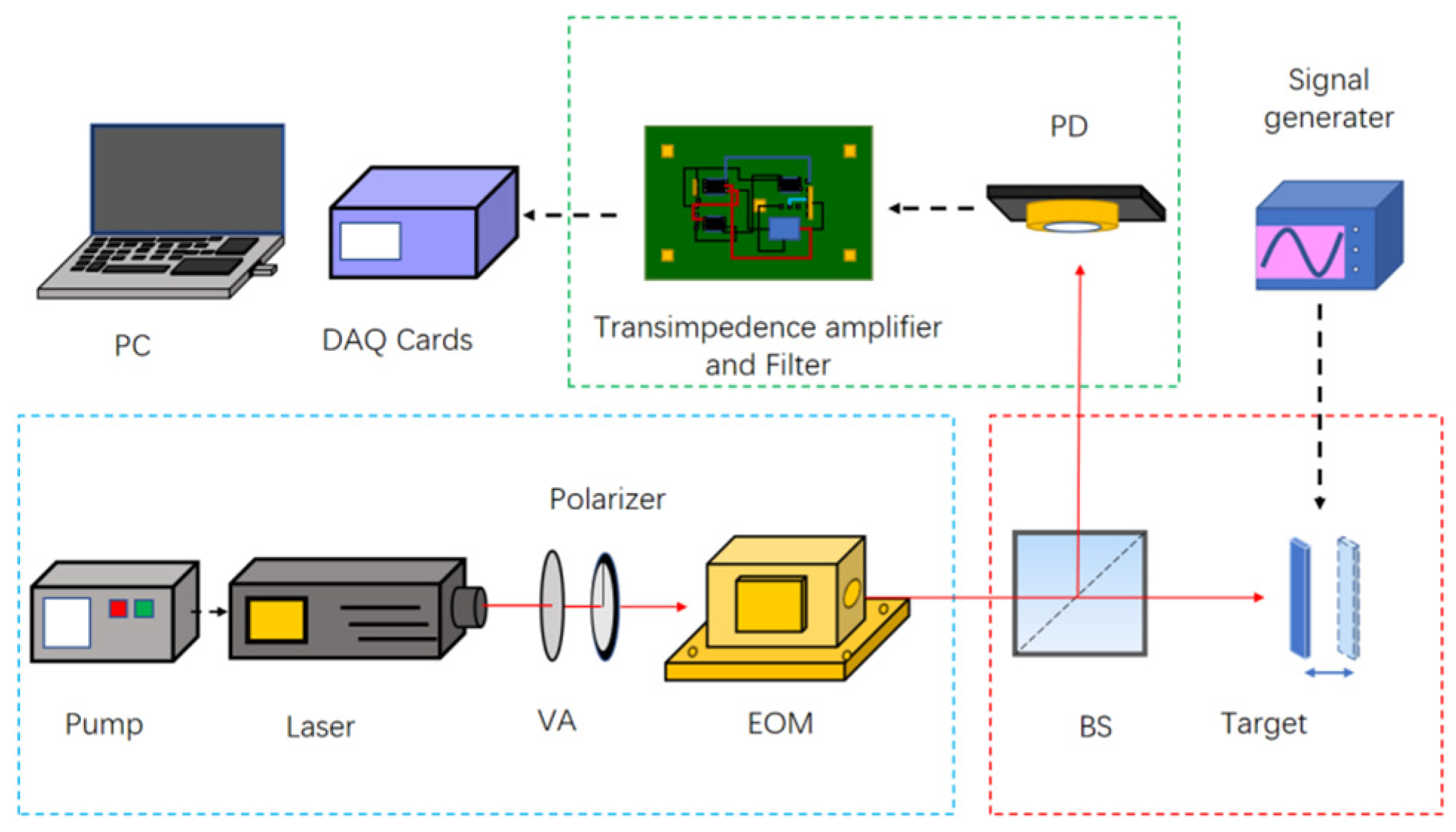
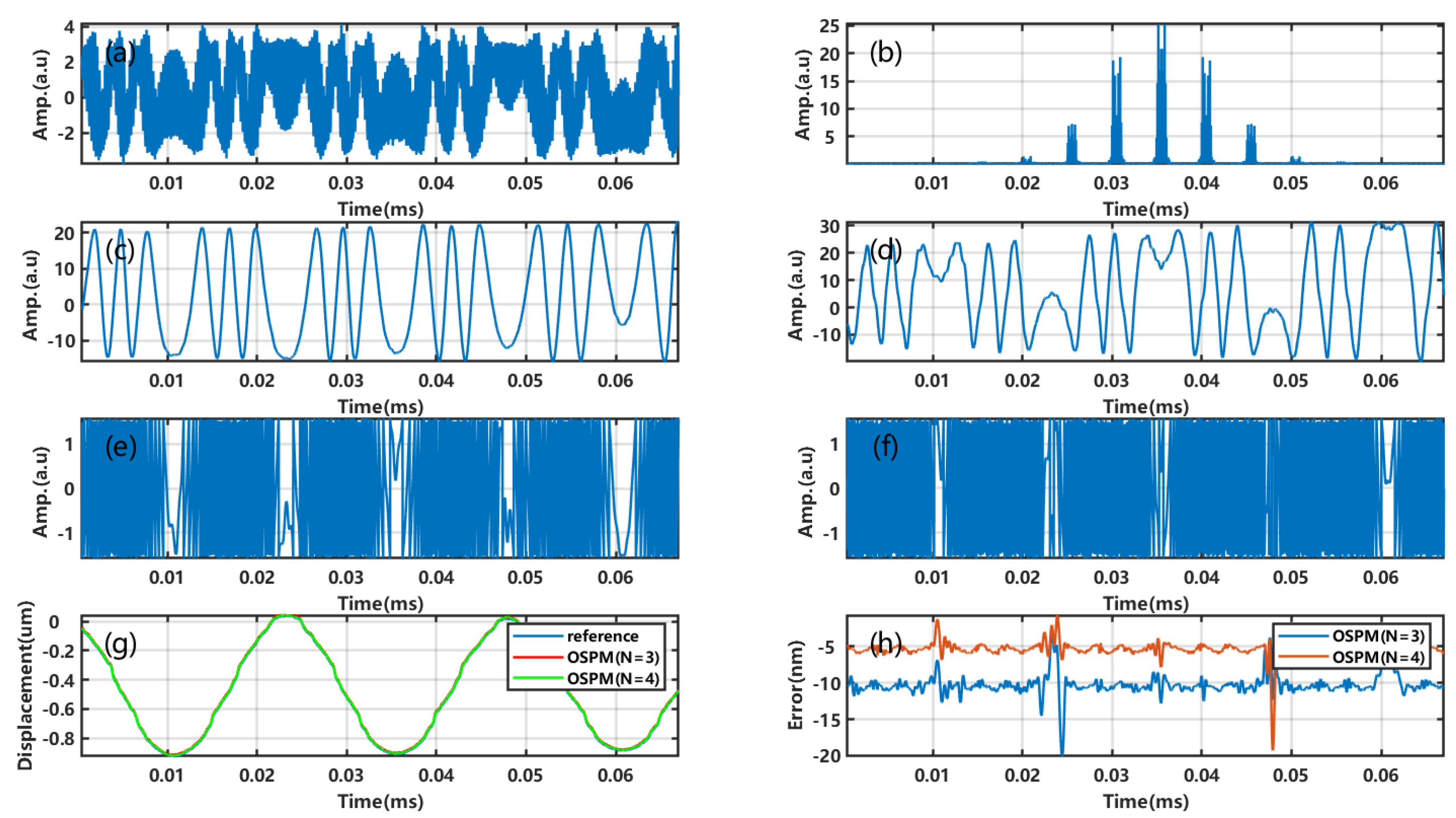
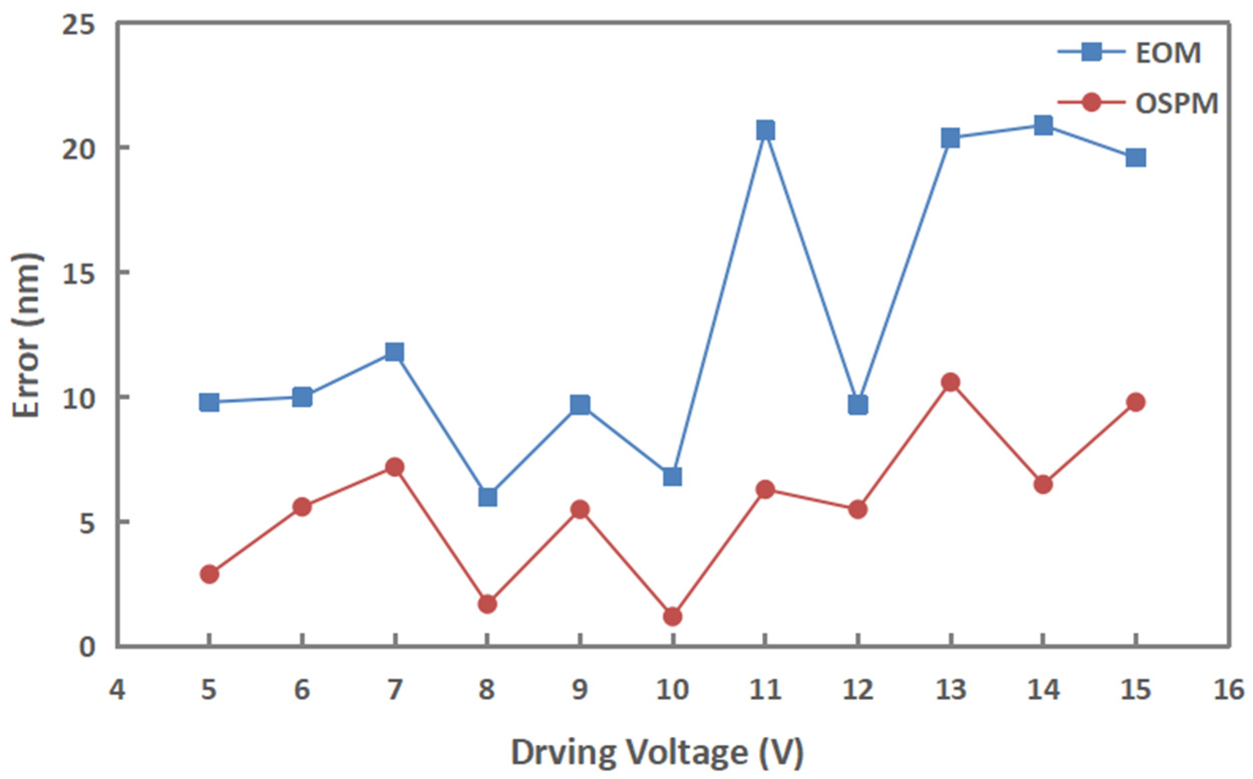
3. Simulations and Experiments

To validate the feasibility of the orthogonal signal phase multiplication algorithm, a series of simulations with varying parameters were conducted based on the analysis above. The parameters involved simulating the harmonic vibration of an external target using amplitude A = 195 nm, frequency f 0 = 80 Hz, and sampling rate f s = 400 kHz. The modulation frequency of the EOM f m is set to 80 kHz, with a modulation depth of 1.67 rad. The remaining parameters were set to λ 0 = 650 nm, α = 5, and = 0.1. The displacement reconstruction process followed the flowchart in Figure 1. The simulated results are presented in Figure 2. Figure 2a shows the phase-modulated SMI signal. First, the signal frequency spectrum was obtained by fast Fourier transform, and the capturing window length was the same as the length of the time domain signal, as shown in Figure 2a. Then, the zero-frequency point was placed in the middle of the spectrum to observe the spectrum conveniently, as shown in Figure 2b. The harmonic components were found to be distributed on both sides of the zero-frequency point with an 80 kHz interval, which is consistent with the theoretical analysis. The first and second harmonics were then extracted using two filters in the frequency domain, followed by using the inverse fast Fourier transform and carriers remove to process the filtered components. The intensities of the harmonics are thus obtained, as shown in Figure 2c,d. Then, we perform the orthogonal signal phase multiplication operation on the first and second harmonics, respectively. Figure 2e,f show the processed signals according by Equations (10) and (11). Apparently, the use of the proposed phase multiplication algorithm resulted in a doubling of the number of fringes between the two flip points. After a phase unwrapping process, the continuous phase variation of the SMI signal was retrieved to reconstruct the motion signal of the external target, as shown in Figure 2g. The results show that the displacement reconstruction error of the proposed method is nearly half that of the conventional EOM method, as shown in Figure 2h.
In order to demonstrate the impact of phase multiplication times N on displacement reconstruction precision, the reconstruction process of N = 2 is simulated without altering any other parameters. The results are shown in Figure 3. Figure 3a–f shows the reconstruction process with N = 1 and N = 2, respectively. It is evident from Figure 3a,d that the fringes of wrapped phase double when the multiplication times are doubled. The reconstructed displacement is given by Figure 3b,e. Figure 3c,f shows the reconstruction error, and the mean square error with N = 2 is approximately 4 nm, which is almost half that of 8.9 nm at N = 1. Theoretically, it can perform more instances of phase multiplication to obtain higher displacement reconstruction precision, but there is no doubt that this will be limited by the modulation frequency. According to the Nyquist sampling theorem, the modulation frequency f m should be more than twice the maximum frequency of the fundamental frequency F m a x .
f m > 2 F m a x
If the external target has a motion L ( t ) = A · s i n 2 π f 0 t , then ϕ F ( t ) = 4 π L ( t ) / λ 0 . The instantaneous frequency F of A 1 ( t ) and A 2 ( t ) can be expressed as follows, where n is the number of phase multiplications:
F = 2 n · 1 / 2 π · d ϕ F ( t ) / d t = 2 n · 4 π A f c o s 2 π f 0 t / λ 0
Combining Equations (13) and (14), the following can be derived:
f m 2 n · 8 π A f 0 / λ 0
From Equation (15), we can see that the measurement range of the system is theoretically limited by the modulation frequency.
To test the effectiveness of the orthogonal signal phase multiplication method, a set of experiments has been conducted using the setup shown in Figure 4. In this experiment, a semiconductor laser (MGL-III-532) is used as the light source, which can emit up to 20 mW of light at 532 nm on single-longitudinal mode and is powered by a constant current supply. To ensure that the SMI system operates under a low-feedback regime, a variable attenuator (VA) was inserted next to the output facet of the LD (laser diode) in the external cavity. The sinusoidal phase modulation was achieved using an electro-optical modulator (EOM, EO-PM-NR-C4) and signal generator (SG, E-610.S0), in combination with a high-voltage amplifier (HVA200). The voltage amplifier has a maximum continuous output current of 100 mA, a voltage gain of 20 times, and a maximum output voltage of ±200 V. A polarizer (P) is inserted after the LD and adjusted in parallel with the EOM active axis to generate a linear polarized light. The external periodic harmonic vibration was provided by PZT (PSt150/5*5/20H, coremorrow), which was driven by a signal generator. The PZT has a movement range of 28 µm with a resolution of 0.15 nm. Changes in laser power were detected by a photodetector (PD) and converted into current, which was then amplified by a transimpedance amplifier (TIA) and acquired by a computer via a data acquisition card (DAQ cards, ISDS205A) with a sampling rate of 1 MS/s. A commercial Doppler interferometer (LV-IS01, SOPTOP, 0.015 nm resolution) was introduced to the detection system as a reference displacement of the PZT to verify the accuracy of the measurement results. A photograph of the experimental setup is shown in Figure 5.
In this experiment, the EOM was operated at a modulation voltage of 6.75 V and modulation frequency of 4 kHz, and the PZT was set to 40 Hz with a driving voltage of 9 V. The proposed OSPM algorithm was used to reconstruct the external vibration displacement, and the results are presented in Figure 6. Figure 6a,b show the modulated SMI signal and its corresponding frequency spectrum. The intensities extracted from the first and second harmonic components are shown in Figure 6c,d. Then, we multiplied the wrapped phase three and four times, and the results are shown in Figure 6e,f. Finally, the reconstructed displacement and the reconstruction error are shown in Figure 6g,h, respectively. It can be seen that the mean square error at N = 4 is approximately 5.4 nm, which is almost half that of 10.6 nm at N = 3.
To further investigate the performance of the OSPM method, reconstruction experiments using the OSPM method were carried out with varying amplitudes. The voltage applied to the PZT was varied from 5 V to 15 V (corresponding amplitude A = 661–2013 nm) in steps of 1 V and multiplication times of N = 4, while all other parameters remained constant. To ensure the accuracy and reliability of the results, the root mean square error (RMSE) of the reconstructions was calculated from multiple measurements. The experimental results, depicted in Figure 7, demonstrate that the reconstruction error of the OSPM method remains consistently below 11 nm, and the maximum relative error of 0.75% occurs at 7V, which is consistently lower than that of the conventional EOM phase modulation method [26]. This provides further evidence of the superiority of the OSPM approach. Getting the higher order Sn and Cn increases the accuracy of the measurements, and the error will increase at the same time. In fact, when the signal-to-noise ratio (SNR) of the SMI signal is high, the increase in the error induced by the higher order Sn and Cn is relatively smaller than the increase in accuracy. When the SNR is low, the error caused by higher-order Sn and Cn is dominant. In short, the SNR will limit the order of Sn and Cn. Because of the modulation, the signal is less affected by low-frequency noise, and we usually do the low-pass filter to improve the SNR to achieve better accuracy.

4. Conclusions

To summarize, our research presents a novel approach that improves the precision of displacement reconstruction by doubling the phase of the orthogonal SMI signal, which obtained from the sinusoidal phase-modulating SMI signal. A detailed explanation of the principle of our proposed method has been provided, and its signal processing procedures are thoroughly described. Both simulated and experimental SMI signals have been utilized to verify the method. The results demonstrate that the reconstruction error is less than 11 nm in the amplitude range from 661 nm to 2013 nm. The experimental results are consistent with the simulations, and the precision can be further improved by performing more rounds of phase multiplication. Application of the orthogonal signal phase multiplication method will promote the application of phase-modulated SMI in displacement measurement with nanometer precision.

Author Contributions

X.W.: conceptualization, methodology, writing—original draft preparation, and funding acquisition. Z.Z.: conceptualization, methodology, investigation, and data curation. H.C. and D.Z.: software, formal analysis, and investigation. T.Z.: investigation and formal analysis. W.H.: conceptualization, methodology, and supervision. All authors have read and agreed to the published version of the manuscript.

Funding

This research was funded by the Natural Science Foundation of Fujian Province (2020J01705), the National Natural Science Foundation of China (11804115), and Enterprise commissioned development project (20223160A0580).

Institutional Review Board Statement

Not applicable.

Informed Consent Statement

Not applicable.

Data Availability Statement

Not applicable.

Conflicts of Interest

The authors declare no conflict of interest.

References

  1. Yang, H.-J.; Deibel, J.; Nyberg, S.; Riles, K. High-precision absolute distance and vibration measurement with frequency scanned interferometry. Appl. Opt. 2005, 44, 3937–3944. [Google Scholar] [CrossRef] [PubMed]
  2. Pfister, T.; Buttner, L.; Czarske, J.; Krain, H.; Schodl, R. Turbo machine tip clearance and vibration measurements using a fibre optic laser Doppler position sensor. Meas. Sci. Technol. 2006, 17, 1693–1705. [Google Scholar] [CrossRef]
  3. Donati, S. Developing self-mixing interferometry for instrumentation and measurements. Laser Photonics Rev. 2012, 6, 393–417. [Google Scholar] [CrossRef]
  4. Chen, W.; Zhang, S.; Long, X. Polarisation control through an optical feedback technique and its application in precise measurements. Sci. Rep. 2013, 3, 1992. [Google Scholar] [CrossRef] [PubMed]
  5. Zhang, Y.; Wang, R.; Wei, Z.; Wang, X.; Xu, H.; Sun, H.; Huang, W. Broad Range and High Precision Self-Mixing Interferometer Based on Spectral Analysis with Multiple Reflections. IEEE Sens. J. 2018, 19, 926–932. [Google Scholar] [CrossRef]
  6. Guo, D.; Wang, M. Self-mixing interferometry based on a double-modulation technique for absolute distance measurement. Appl. Opt. 2007, 46, 1486–1491. [Google Scholar] [CrossRef]
  7. Duan, Z.; Yu, Y.; Gao, B.; Jiang, C. Absolute distance measurement based on multiple self-mixing interferometry. Opt. Commun. 2017, 389, 270–274. [Google Scholar] [CrossRef]
  8. Kou, K.; Wang, C.; Liu, Y. All-phase FFT based distance measurement in laser self-mixing interferometry. Opt. Lasers Eng. 2021, 142, 106611. [Google Scholar] [CrossRef]
  9. Li, L.; Zhang, Y.; Zhu, Y.; Dai, Y.; Zhang, X.; Liang, X. Absolute Distance Measurement Based on Self-Mixing Interferometry Using Compressed Sensing. Appl. Sci. 2022, 12, 8635. [Google Scholar] [CrossRef]
  10. Donati, S.; Rossi, D.; Norgia, M. Single Channel Self-Mixing Interferometer Measures Simultaneously Displace0ment and Tilt and Yaw Angles of a Reflective Target. IEEE J. Quantum Electron. 2015, 51, 1–8. [Google Scholar] [CrossRef]
  11. Zhao, Y.; Zhang, H. Angle measurement method based on speckle affected laser self-mixing interference signal. Opt. Commun. 2021, 482, 126569. [Google Scholar] [CrossRef]
  12. Xu, X.; Dai, Z.; Wang, Y.; Li, M.; Tan, Y. High Sensitivity and Full-Circle Optical Rotary Sensor for Non-Cooperatively Tracing Wrist Tremor with Nanoradian Resolution. IEEE Trans. Ind. Electron. 2021, 69, 9605–9612. [Google Scholar] [CrossRef]
  13. Wang, X.; Yuan, Y.; Chen, P.; Gao, B. Laser self-mixing based on peak–valley point detection algorithm for displacement reconstruction. Opt. Quantum Electron. 2020, 52, 34. [Google Scholar] [CrossRef]
  14. Amin, S.; Zabit, U.; Bernal, O.D.; Hussain, T. High Resolution Laser Self-Mixing Displacement Sensor Under Large Variation in Optical Feedback and Speckle. IEEE Sens. J. 2020, 20, 9140–9147. [Google Scholar] [CrossRef]
  15. Wang, Y.; Li, Y.; Xu, X.; Tian, M.; Zhu, K.; Tan, Y. All-fiber laser feedback interferometry with 300 m transmission distance. Opt. Lett. 2021, 46, 821–824. [Google Scholar] [CrossRef]
  16. Ge, S.; Lin, Y.; Chen, H.; Kong, X.; Zhu, D.; Dong, Z.; Wang, X.; Huang, W. Signal extraction method based on spectral processing for a dual-channel SMI vibration sensor. Opt. Lasers Eng. 2023, 164, 107531. [Google Scholar] [CrossRef]
  17. Wu, S.; Wang, D.; Xiang, R.; Zhou, J.; Ma, Y.; Gui, H.; Liu, J.; Wang, H.; Lu, L.; Yu, B. All-Fiber Configuration Laser Self-Mixing Doppler Velocimeter Based on Distributed Feedback Fiber Laser. Sensors 2016, 16, 1179. [Google Scholar] [CrossRef]
  18. Jiang, C.; Geng, Y.; Liu, Y.; Liu, Y.; Chen, P.; Yin, S. Rotation velocity measurement based on self-mixing interference with a dual-external-cavity single-laser diode. Appl. Opt. 2019, 58, 604–608. [Google Scholar] [CrossRef]
  19. Wang, X.; Yang, H.; Hu, L.; Li, Z.; Chen, H.; Huang, W. Single Channel Instrument for Simultaneous Rotation Speed and Vibration Measurement Based on Self-Mixing Speckle Interference. IEEE Photonics J. 2021, 14, 6802405. [Google Scholar] [CrossRef]
  20. Tan, Y.; Zhang, S.; Xu, C.; Zhao, S. Inspecting and locating foreign body in biological sample by laser confocal feedback technology. Appl. Phys. Lett. 2013, 103, 101909. [Google Scholar] [CrossRef]
  21. Zhao, Y.; Xu, G.; Zhang, C.; Liu, K.; Lu, L. Vibration displacement immunization model for measuring the free spectral range by means of a laser self-mixing velocimeter. Appl. Opt. 2019, 58, 5540–5546. [Google Scholar] [CrossRef] [PubMed]
  22. Zhou, B.; Wang, Z.; Shen, X.; Zhang, L.; Tan, Y. High-sensitivity laser confocal tomography based on frequency-shifted feedback technique. Opt. Lasers Eng. 2020, 129, 106059. [Google Scholar] [CrossRef]
  23. Liu, B.; Ruan, Y.; Yu, Y. Determining System Parameters and Target Movement Directions in a Laser Self-Mixing Interferometry Sensor. Photonics 2022, 9, 612. [Google Scholar] [CrossRef]
  24. Donati, S.; Giuliani, G.; Merlo, S. Laser diode feedback interferometer for measurement of displacements without ambiguity. IEEE J. Quantum Electron. 1995, 31, 113–119. [Google Scholar] [CrossRef]
  25. Bes, C.; Plantier, G.; Bosch, T. Displacement Measurements Using a Self-Mixing Laser Diode Under Moderate Feedback. IEEE Trans. Instrum. Meas. 2006, 55, 1101–1105. [Google Scholar] [CrossRef]
  26. Guo, D.; Wang, M.; Tan, S. Self-mixing interferometer based on sinusoidal phase modulating technique. Opt. Express 2005, 13, 1537–1543. [Google Scholar] [CrossRef]
  27. Guo, D. Quadrature demodulation technique for self-mixing interferometry displacement sensor. Opt. Commun. 2011, 284, 5766–5769. [Google Scholar] [CrossRef]
  28. Xia, W.; Wang, M.; Yang, Z.; Guo, W.; Hao, H.; Guo, D. High-accuracy sinusoidal phase-modulating self-mixing interferometer using an electro-optic modulator: Development and evaluation. Appl. Opt. 2013, 52, B52–B59. [Google Scholar] [CrossRef]
  29. Ali, N.; Zabit, U.; Bernal, O.D. Nanometric Vibration Sensing Using Spectral Processing of Laser Self-Mixing Feedback Phase. IEEE Sens. J. 2021, 21, 17766–17774. [Google Scholar] [CrossRef]
  30. Lu, L.; Hu, L.; Li, Z.; Qiu, L.; Huang, W.; Wang, X. High Precision Self-Mixing Interferometer Based on Reflective Phase Modulation Method. IEEE Access 2020, 8, 204153–204159. [Google Scholar] [CrossRef]
  31. De Groot, P.J.; Gallatin, G.M.; Macomber, S.H. Ranging and velocimetry signal generation in a backscatter-modulated laser diode. Appl. Opt. 1988, 27, 4475–4480. [Google Scholar] [CrossRef] [PubMed]
  32. Cui, X.; Liu, Y.; Chen, P.; Li, C. Measuring two vibrations using dual-external-cavity structure in a self-mixing system. Opt. Lasers Eng. 2021, 141, 106557. [Google Scholar] [CrossRef]
Figure 1. Flow chart of the method.
Photonics 10 00575 g001
Figure 2. Realization of interference signal processing. (a) Simulated phase modulating SMI signal. (b) Frequency spectrum of SMI signal. (c) Intensity of the first harmonic, S 1 ( t ) . (d) Intensity of the second harmonic, C 1 ( t ) . (e) The first harmonic with phase multiplication, S 2 ( t ) . (f) The second harmonic with phase multiplication, C 2 ( t ) . (g) Reconstructed displacement. (h) Displacement reconstruction error.
Photonics 10 00575 g002
Figure 3. Displacement reconstruction results with N = 1 and N = 2. (a) Extracted phase from SMI signal (N = 1). (b) Reconstructed displacement (N = 2). (c) Displacement reconstruction error (N = 1). (d) Extracted phase from SMI signal (N = 2). (e) Reconstructed displacement (N = 1). (f) Displacement reconstruction error (N = 2).
Photonics 10 00575 g003
Figure 4. Diagram of experimental setup. The blue, red, and green boxes are the optical path module, external target module, and circuit processing module, respectively.
Photonics 10 00575 g004
Figure 5. Photograph of experimental setup. The blue, red, and green boxes are the optical path module, external target module, and circuit processing module, respectively.
Photonics 10 00575 g005
Figure 6. Experimental results. (a) Simulated phase modulating SMI signal. (b) Frequency spectrum of SMI signal. (c) Intensity of the first harmonic. (d) Intensity of the second harmonic. (e) Extracted phase from SMI signal (N = 3). (f) Extracted phase from SMI signal (N = 4). (g) Reconstructed displacement. (h) Displacement reconstruction error.
Photonics 10 00575 g006
Figure 7. Experimental RMS errors of reconstruction based on the proposed OSPM method (in red), and the conventional EOM methods (in blue) with different driving voltages.
Photonics 10 00575 g007
Disclaimer/Publisher’s Note: The statements, opinions and data contained in all publications are solely those of the individual author(s) and contributor(s) and not of MDPI and/or the editor(s). MDPI and/or the editor(s) disclaim responsibility for any injury to people or property resulting from any ideas, methods, instructions or products referred to in the content.

