1. Introduction
Taking a weakness of one system and turning it into a strength in a different application is a powerful and creative approach to finding new technological innovations. A striking example of this approach is the maximization of axial wavelength dispersion in a lens system which is highly undesirable in classical imaging systems. This working principle is used for example in confocal microscopes [
1,
2], endoscopy [
3], thickness measurement [
4,
5], surface profiling [
6] or tunable light sources [
7]. To achieve high system performance in these applications, the equivalent Abbe number must be as low as possible. The equivalent Abbe number is the Abbe number that a glass of a thin single lens would have to achieve the same chromatic aberration of the complete optical system [
8]. The smaller the Abbe number, the larger the axial wavelength spread becomes. When the equivalent Abbe number of a lens group is lower than the lowest Abbe number of the optical elements involved, the system is said to be hyperchromatic. The introduction should briefly place the study in a broad context and highlight why it is important. It should define the purpose of the work and its significance.
The aim of achieving optical systems with large axial chromatic focus shifts has already been the subject of various studies. Hillenbrand [
9] demonstrated certain design strategies for developing hybrid hyperchromats aiming at large longitudinal chromatic aberrations. However, the approach presented here has only been proven for a hybrid system and a purely diffractive system. Purely refractive systems have been neglected, and the influence of lens materials on axial color distribution has not been addressed. Zhang et al. [
10] presented various doublets that are suitable for the creation of hyperchromatic systems. The doublets discussed are only used in combination with other optical elements and the systems are not optimized for imaging spot quality. For their study, the authors used only refractive components and the choice of materials is only qualitative and not formula based. In our preliminary work [
11], we investigated purely refractive and hybrid doublet systems with the aim of obtaining extremely low equivalent Abbe numbers. However, this article did not consider certain layout variants such as purely diffractive systems, nor did it consider the possibility of using a distance between the lenses and dimensioning it appropriately to further reduce the equivalent Abbe number.
This paper investigates how previously neglected lens configurations, especially lens spacing, allow the development of stronger hyperchromatic effects. As a verification of this assumption, the calculation of the equivalent Abbe number in the paraxial region is shown in
Section 2 of this paper. The calculation is based on the focal lengths, the Abbe numbers of the materials and the distance between the optical components. Using paraxial assumptions, it is possible to obtain approximate solutions that are sufficient for a qualitative assessment of the behavior of different hyperchromats and are suitable as starting parameters for subsequent optimizations. Based on these evaluations, a three-step procedure was used to achieve a minimum equivalent Abbe number for lens combinations. For the first step in
Section 3 and
Section 4, numerical calculations were performed with respect to geometric constraints to determine the smallest possible equivalent Abbe number of an optical system. The second and third steps in
Section 5 and
Section 6 take into account additional geometric constraints such as the radii, diameters and thicknesses of the lenses. The results of these numerical calculations are transferred to the optical design program “Zemax OpticStudio” and optimized with respect to aberrations and geometric limits. These considerations have been carried out for purely refractive, purely diffractive and hybrid systems combining refractive and diffractive elements.
2. Paraxial Consideration of the Equivalent Abbe Number for the Refractive, Diffractive and Hybrid Cases
To achieve a low equivalent Abbe number for a hyperchromat, it is necessary to study the influencing variables that are implemented in the calculation. The equivalent Abbe number
is the quotient of the focal length
of the system and the longitudinal chromatic aberration
[
12].
The required focal length of the entire optical system, consisting of two separate elements, is easily calculated from the partial focal lengths of the individual elements
and the distance
between them [
13].
In this contribution, the chromatic focal shift
was calculated from the difference between the image distances of the second lens for the short
and long reference wavelengths
[
14].
These image distances were calculated for the short reference wavelength (
= 486.13 nm) and for the long reference wavelength (
= 656.27 nm) of the optical system at an object distance of infinity [
15]. In addition, the calculations in Formulas (4) and (5) use the total focal length of the system
and the focal length of the first lens
at the corresponding wavelength.
The focal lengths of the two lenses
are defined only for the central reference wavelengths (
= 587.56 nm). For different wavelengths, the focal lengths of a thin lens are calculated from the corresponding refractive indices
and their lens radii
[
16]:
By substituting Formula (6) into Formulas (7) and (8), the dependence on the lens radii is eliminated and the change in focal length can be computed as follows:
To calculate the different refractive indices for different wavelengths, the assumptions in Formulas (11) and (12) were defined. In the formulas the refractive indices for the reference wavelengths
are obtained by using the refractive index for the center wavelength
and the difference between the refractive indices of the longest and shortest wavelengths
. The errors resulting from these assumptions are small enough to be negligible for paraxial considerations. However, in the later
Section 5 and
Section 6, the real dispersion curves of the materials are used for the optimizations to make the results even more accurate.
Furthermore, the Abbe numbers of the optical elements are needed to calculate the wavelength-dependent refractive indices. The Abbe numbers for refractive lenses
are material dependent and usually have a positive value, meaning that the lenses have higher focal lengths for longer wavelengths and are calculated using the refractive indices. For optical glasses, achievable values range from 8 for zinc selenide to 95 for calcium fluoride [
17,
18].
If the longitudinal chromatic aberration is to be investigated outside the reference wavelength range from
to
, the Abbe number must be modified [
19].
,
and
are the refractive indices at the center, shortest and longest wavelengths, respectively.
In contrast to refractive elements, diffractive optical elements exhibit an inverse dispersion, which is independent of the material and always results in a constant value for the Abbe number. It can be obtained from the middle
, the shortest
and the longest wavelength
of the spectral range [
20]. For the visible spectral range, the Abbe number for diffractive elements is −3.45. The very low absolute value of the Abbe number and the associated high dispersion effect make them very interesting for the design of hyperchromats.
If Formula (13) is rearranged according to the refractive index difference
and substituted into Formulas (11) and (12), then the refractive indices at the reference wavelengths can be calculated as follows:
By inserting the Formula (16) to (9) and Formula (17) to (10), the focal lengths of the lenses
at the different wavelengths
can be computed using only the Abbe number
and the central focal length
.
The next section examines the factors that influence the equivalent Abbe number of a two-element system. For this purpose, the axial color separation achieved for different configurations will be the subject of consideration and discussion. The aim is to find the optimal settings for a variety of optical systems with extremely low equivalent Abbe numbers.
3. Investigation of Optical Key Factors for Purely Refractive Optical Systems
As mentioned before, the equivalent Abbe number in the paraxial region for a two-element system depends on the Abbe numbers of the lens materials, the focal lengths of the individual lenses and the distance between them.
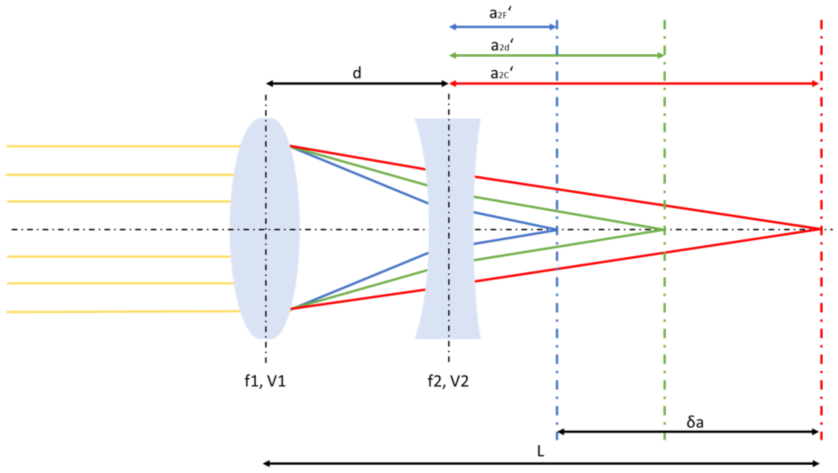
Figure 1 shows the schematic of the lens configuration and indicates the characteristic quantities. Here
is the distance between the lenses and
,
,
and
are the corresponding focal lengths and Abbe numbers. The total length of the system
is defined as the distance between the principal plane of the first lens and the system’s focal position with the largest distance to the lens combination. Depending on the sign of the equivalent Abbe number, negative or positive, the focus position with the largest distance correlates with the shortest or the longest wavelength. The image distances of the configuration for the defined wavelengths are denoted by
,
and
and refer to the principal plane of the second lens. The axial chromatic shift
is indicated by the difference between
and
.
For the following simulations, some plausibility assumptions are made for the determination of extremely small equivalent Abbe numbers. First, the focal lengths of the two lenses varied from −100 mm to −10 mm and from +10 mm to +100 mm. Since the overall system should have a sufficiently large numerical aperture, it is also necessary to aim for large lens diameters. For large diameters, however, it is difficult to achieve small focal lengths, so a lower absolute limit is considered here. In addition, four different lens materials have been selected, including both standard lenses widely used in optical systems and special materials with extreme dispersion properties. P-SF68 [
21] and N-FK51 [
22], which have the lowest and highest Abbe numbers, respectively, among conventional glasses that can be molded by precision molding [
23], were selected as standard materials. As unconventional materials, ZnSe and CaF
2 were selected which have extremely low and high Abbe numbers but are still suitable as lens materials.
To introduce an appropriate reference length, only solutions with a total system length of 100 mm or less are considered. Furthermore, potential results are limited to optical systems with positive focal lengths over the entire wavelength range. In addition, the image distances of the smallest and longest wavelengths must be positive to ensure that the chromatic focal shift occurs behind the lenses.
After defining the boundary criteria, the next step is to investigate the effect of the distance between the two lenses on the absolute equivalent Abbe number. Here, the combinations of lenses with different Abbe numbers are considered. For this purpose, a software code was written in Matlab [
24] using Formulas (1) – (5) with the introduced assumptions. For each lens distance (varied in 0.1 mm increments) and material combination, the focal lengths of the two lenses were varied in 0.1 mm increments and the lowest attainable equivalent Abbe number was determined. The maximum lens distance considered was limited by the maximum total system length of 100 mm. In total, the equivalent Abbe numbers of about three billion different optical systems are calculated and studied for each material combination (=3 × 10
6 focal length combinations × 10
3 lens distances).
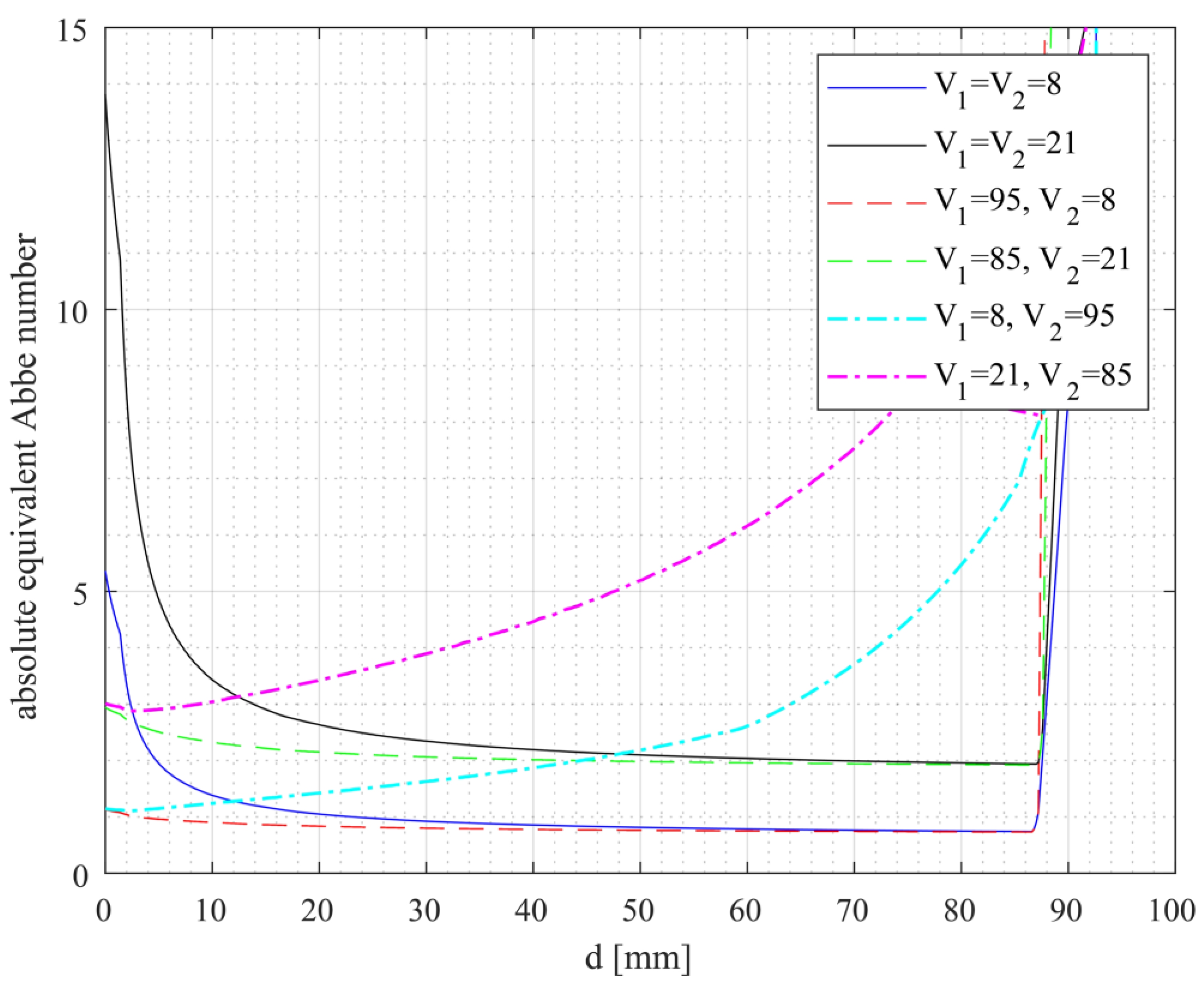
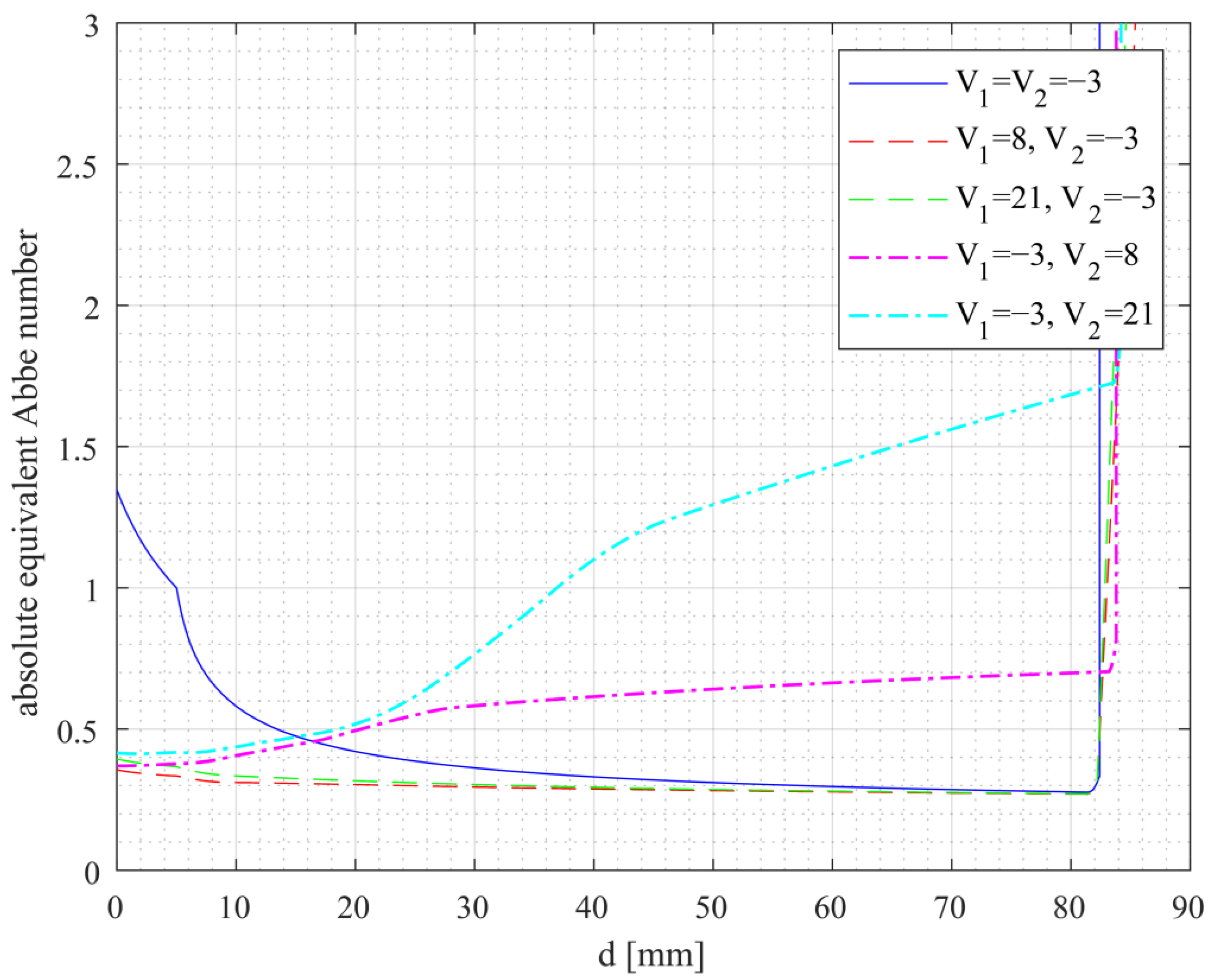
Figure 2 shows the graphs for the smallest possible absolute equivalent Abbe numbers as a function of the distance between the lenses. In the figure, three different types of lines are displayed which belong to the following Abbe number ratios: solid lines: V
1 = V
2; dashed lines: V
1 > V
2; dotted-dashed lines: V
1 < V
2.
Figure 2 shows that the optimum distance corresponding to a minimum equivalent Abbe number depends on the ratio of the Abbe numbers of the first and second lenses. If both Abbe numbers are equal (solid lines), the distance between these two elements should be very large. If the Abbe number of the first element is smaller than that of the second (dotted-dashed lines), the distance should be as small as possible. In the case where the first Abbe number is larger than the second (dashed lines), the influence of the distance is small and only a slight decrease in the equivalent Abbe number is observed at large distances. In addition to determining the optimum lens distance,
Figure 2 also allows the selection of the appropriate material for hyperchromatic lenses. The smallest equivalent Abbe numbers over a large lens distance range are obtained for a combination of a high value for the Abbe number of the first element and a small value for the second element. However,
Figure 2 also shows that for a properly chosen distance, it is only important that one of the lenses’ Abbe numbers is as small as possible. Therefore, all combinations, including the material with an Abbe number of eight, achieve almost the same lowest absolute equivalent Abbe number of 0.8 but at different distances. For distances above 90 mm, the equivalent Abbe number rises sharply for all curves. This is due to the fact that the condition of a total length of less than 100 mm cannot be met with a positive and negative lens, but only if both focal lengths have positive values. However, this configuration is not suitable for forming highly dispersed systems. In summary,
Figure 2 shows that one lens should have an Abbe number as low as possible and the other as high as possible. Alternatively, both lenses should have very low Abbe numbers.
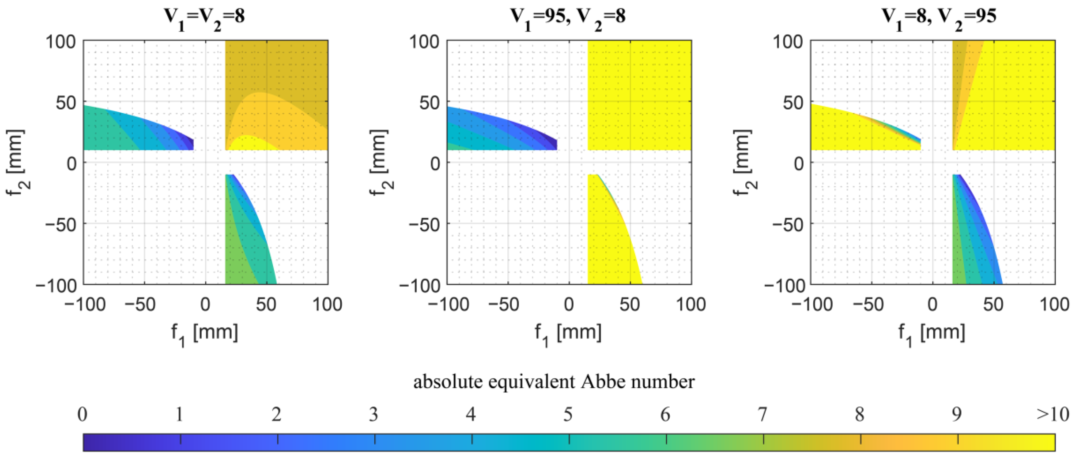
As explained above, the minimum values of the equivalent Abbe number were examined in a general overview; the concrete influence of the focal lengths of the individual lenses was not considered. To analyze the influence of the focal lengths, three combinations of Abbe numbers for both lenses were used: V
1 = V
2, V
1 > V
2 and V
1 < V
2. For these configurations, the material combinations with the lowest achievable equivalent Abbe numbers from
Figure 2 were used. As a reference, the lens distance was set to 15 mm because all configurations in
Figure 2 achieve small equivalent Abbe numbers at this distance. A self-coded script varied the focal lengths
and calculated the absolute equivalent Abbe number for each focal length combination. Each of the plots in
Figure 3 shows the results for a particular combination of Abbe numbers. The absolute equivalent Abbe number obtained is shown as a function of the focal length in a color-coded graph. The darker the color in the diagram, the lower the equivalent Abbe number. Equivalent Abbe numbers greater than 10 are shown in yellow.
From
Figure 3, it can be seen that the choice of the focal length of the lenses as well as the choice of the distance depends on the ratio of the Abbe numbers. For the combination where both Abbe numbers are equal, the lowest absolute equivalent Abbe numbers are obtained with a positive first lens and a negative second lens. With the same choice of focal lengths, it is also possible to obtain low absolute equivalent Abbe numbers if the second Abbe number is smaller than the first. In the reverse case, if the first Abbe number is smaller, the focal length
should be positive and
should be negative. Any configuration with a positive focal length
less than the lens distance will result in a negative unusable image distance. Thus, the value of the first focal length must always be higher than the distance between the lenses. Since the combination of two negative focal lengths always results in a negative total focal length, these combinations can also be excluded. In the case where both focal lengths are positive, only very high values of the equivalent Abbe number (>8) are obtained. It can also be seen that the resulting equivalent Abbe number is more sensitive to changes in the focal length of the lens with the lower Abbe number than to changes in the focal length of the material with the higher Abbe number. When both Abbe numbers are equal, the magnitude of the first focal length is more important than the second.
From the study of the parameters that affect the equivalent Abbe number of a refractive system, it can be concluded that the choice of focal length and lens distance depends on the ratio of Abbe numbers. Regardless of the ratio of the Abbe numbers, it is necessary to select one material with the highest possible Abbe number and a second material with the lowest possible Abbe number to obtain the lowest possible values for the equivalent Abbe number of the optical system. Furthermore, the lens with the higher Abbe number should have a negative focal length and the other element with the lower Abbe number should have a positive focal length. It is also important to note that if the focal length of the first lens is positive, the lens distance should be very short, and if the focal length of the first lens is negative, the lens distance should be very long. All of these conditions are also valid for standard lens materials with moderate Abbe numbers. The most important finding, however, is that refractive systems have the potential to achieve much lower equivalent Abbe numbers than single diffractive elements with values as low as 0.8 through sophisticated designs.
4. Investigation of Optical Key Factors for Purely Diffractive and Hybrid Optical Systems
In this section, the optimum design parameters for optical systems including diffractive elements will be discussed. It is expected that the use of DOEs will result in a large reduction in the equivalent Abbe number, since the absolute Abbe number of diffractive elements is much lower than that of refractive elements. The procedure for studying the factors influencing the equivalent Abbe number for hybrid and purely diffractive systems follows the one discussed previously for purely refractive systems. The same preconditions were used as in the previous chapter.
For the initial consideration of the influence of the distance between the two elements, five different combinations were investigated. Each of these combinations had at least one diffractive element. As before, the distance and the two focal lengths
and
were varied for these different combinations. Again, the lowest absolute equivalent Abbe number for varying focal lengths
and
was calculated for each distance.
Figure 4 shows the resulting minimum absolute Abbe number as a function of element spacing for all five combinations. In the legend, the value of V = −3 for the Abbe number indicates the DOE. For the different curves, the same presentation is chosen as before: solid lines: V
1 = V
2; dashed lines: V
1 > V
2; dotted-dashed lines: V
1 < V
2.
As with purely refractive systems, the shape of the curves depends on the ratio of the Abbe numbers. With a first diffractive and a second refractive element (dotted and dashed lines), the smallest equivalent Abbe numbers are achieved at very small distances. In contrast, two diffractive lenses (solid line) result in small equivalent Abbe numbers for large distances. With a refractive lens as the first element and a DOE as the second element (dashed lines), the value of the absolute equivalent Abbe number remains nearly constant with a slight decrease at long distances. The small differences between the dashed and dotted-dashed lines also suggest that the Abbe number of the refractive lens has only a minor effect. As expected, the axial color separation of these hybrid and purely diffractive systems is significantly greater than that of purely refractive systems. It should be noted that under the condition of limiting the total length of the system to a maximum of 100 mm, it is not possible to implement configurations with small equivalent Abbe numbers for lens distances greater than 86 mm.
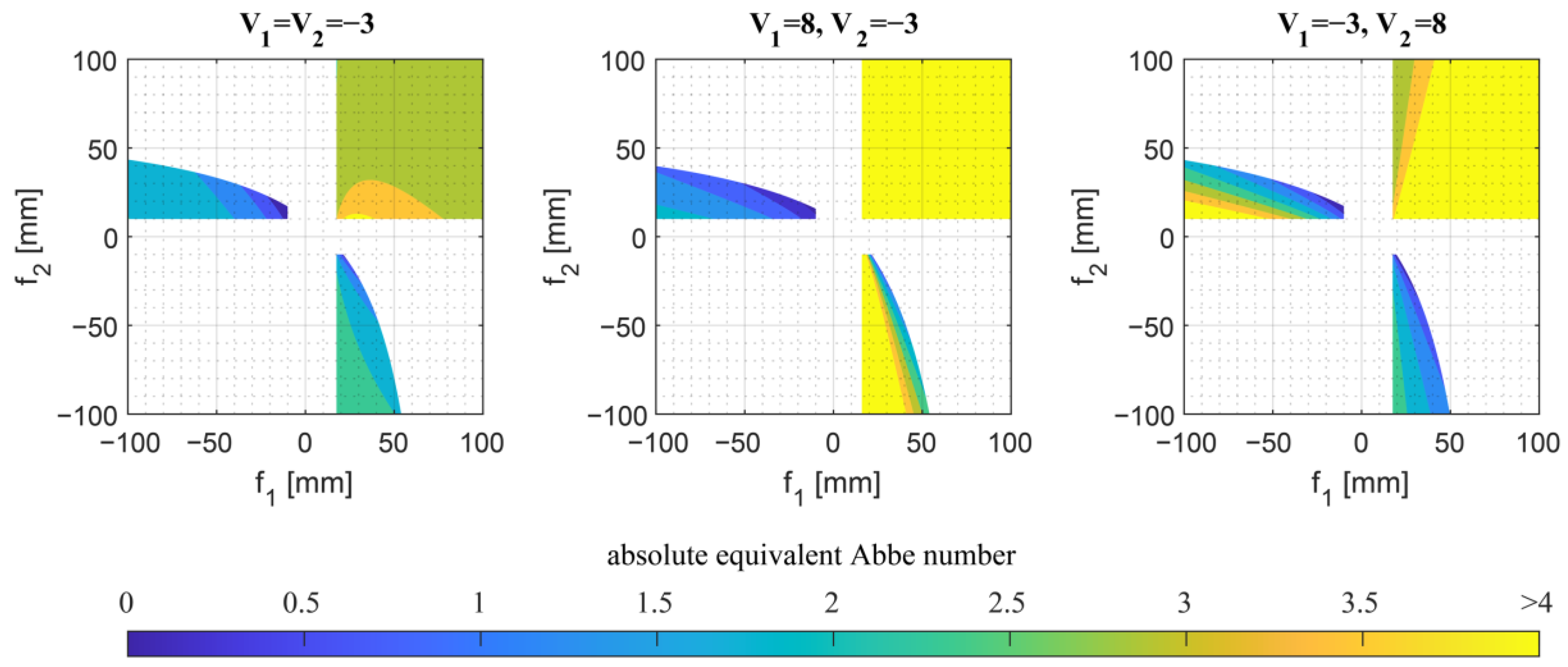
After analyzing the dependence of the equivalent Abbe numbers on the distance between the lenses in refractive–diffractive systems, the influence of the focal length will be examined in the
Figure 5. Again, three different configurations were investigated, differing in the number of diffractive elements and the sequence of the diffractive and refractive optics. As a reference, the distance between the two elements was set to 15 mm, resulting in small values for the equivalent Abbe number for all curves in
Figure 4. The equivalent Abbe number was calculated by software code for each pair of focal lengths. The color scale ranges from blue for very small equivalent Abbe numbers to yellow for the upper limit (>4).
The plots for the different Abbe number combinations show very similar behavior to the ones of the purely refractive systems. Again, the choice of two positive focal lengths is not useful because the absolute equivalent Abbe numbers are highest in the first quadrant of all diagrams. Furthermore, the combination of two focal lengths from the third quadrant does not yield useful results, because it is impossible to achieve a positive total optical power with two negative lenses. When two diffractive elements are used, the minimum absolute equivalent Abbe numbers occur in the second quadrant and very low values are still obtained in the fourth quadrant. It is, therefore, possible to select a positive or negative value for the first focal length in combination with an inverted focal length for the second lens. If only the second element is diffractive, the first focal length should be negative and the second positive. In the case where only the first element is diffractive, the lowest absolute equivalent Abbe numbers are obtained for a positive focal length and a negative focal length .
The results of this chapter have shown that the hybrid and purely diffractive systems have great potential to achieve equivalent Abbe numbers that are much smaller than those of the purely refractive systems with values as low as 0.3. However, it is important to know how to dimension the individual parameters in order to take advantage of this potential. As a general rule, when designing hyperchromatic hybrid systems, the DOE should have a positive focal length and the refractive element a negative focal length. Although the Abbe number of a refractive lens should be as low as possible, choosing a material with a higher Abbe number has been shown to have little effect on the hyperchromia of the system if the lens distance and focal lengths are chosen correctly. Therefore, it is suggested that for these systems it is more important to choose a material with a high refractive index for the refractive element rather than a low Abbe number in order to achieve shorter focal lengths without increasing spherical aberration.
5. Numerical Finding of Global Minima and Optimization for Refractive System
In the previous chapters, the design of extreme hyperchromatic systems was treated using a straightforward qualitative paraxial approach. Important aspects such as lens diameters and thicknesses, which are necessary for real implementation, were not taken into account. To substantiate these results, the quantitative parameters of a double lens system with the lowest possible equivalent Abbe number are determined by numerical calculation using a software code programmed in Matlab. The results are then transferred to an optical design program where they are optimized for aberrations and geometric conditions.
The wavelength range considered extends from
to
so that the corresponding Abbe numbers for the materials involved can also be used. To limit the possible results, the maximum total axial length of the system is again 100 mm with an entrance pupil diameter of 10 mm. As an additional filter, a minimum f-number of eight was specified to prevent large spherical aberrations that cannot be adequately corrected by a two-lens system with spherical surfaces [
25]. Since the previous considerations indicate that small equivalent Abbe numbers are expected at small focal lengths, the maximum focal length
was limited to 100 mm. The minimum focal length
was derived from the minimum radius of the lens
and the refractive index of the lens material
(
= 1,2; first and second lenses). The following formula assumes a thin biconvex lens shape for positive lenses and a biconcave for negative lenses.
The minimum radius
of such a lens with a fixed lens thickness
can be achieved if the lens diameter
and the edge thickness
are as small as possible. Geometric conditions, such as the minimum lens diameter of 5 mm and the minimum edge thickness of 1 mm, have been defined, taking into account the manufacturing limits of standard lenses [
26].
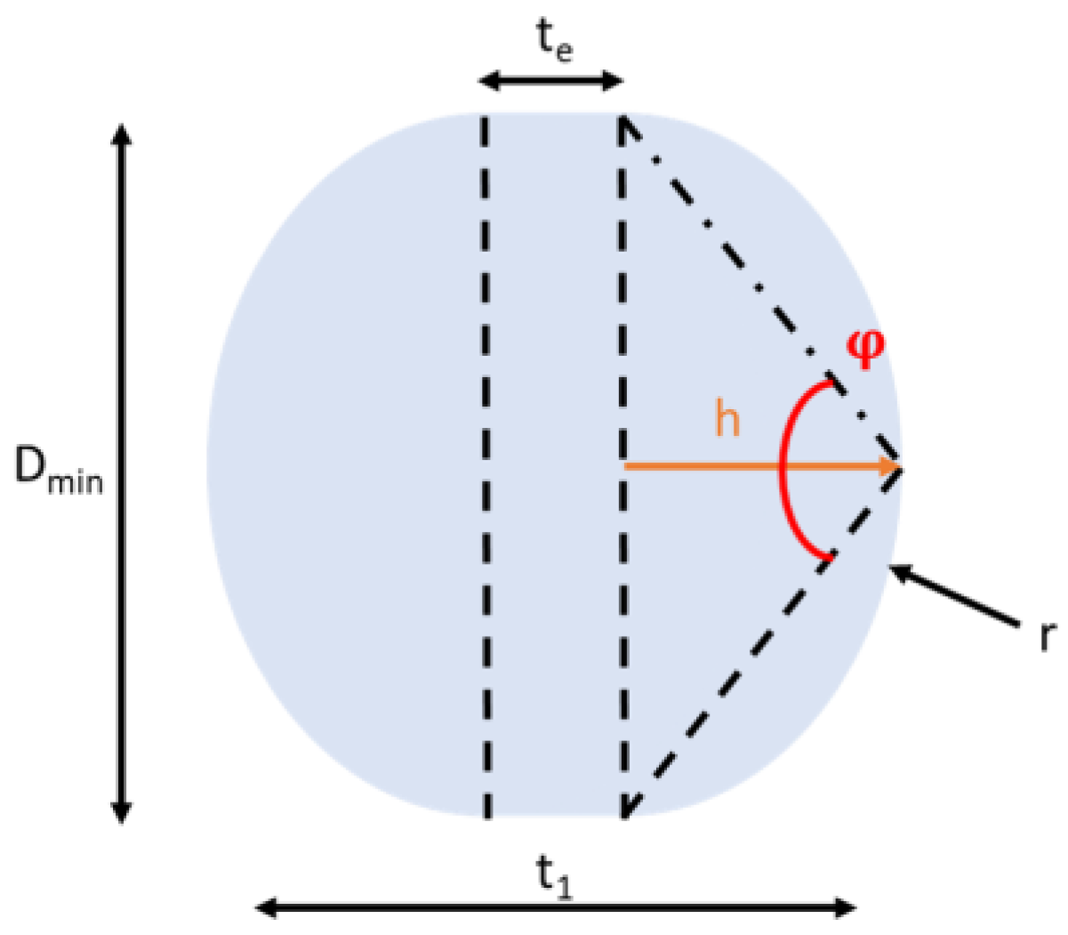
Figure 6 shows a biconvex lens with the values needed to describe its shape.
The smallest possible radius of such a lens can be calculated from the angle of the isosceles triangle
spanned by the radius of curvature and the minimum lens diameter
using the chord theorem [
27]. The minimum diameter of the first lens was assumed to be the diameter of the entrance pupil, and a minimum diameter of 5 mm was used for the second lens.
The angle
is obtained from trigonometric conditions using the sag height of the curvature
and the diameter of the lens
.
From the minimum edge thickness
and the lens thickness
, the curvature height
can be calculated.
By substituting Formulas (22) and (23) into Formula (21), the smallest possible radius of a biconvex lens
is obtained as a function of the minimum lens diameter
, the minimum edge thickness
and the lens thickness
.
In order to find the optimum layout, the program computes the values for the focal lengths
and the distance
for the lowest equivalent Abbe number. All the constraints considered and defined for the design are listed in
Table 1:
Using the defined limits, the program combines all possible focal lengths for each distance varied from 0 to 50 mm in steps of 0.1 mm and calculates the equivalent Abbe numbers. For these calculations, Formulas (1) through (5) have been implemented in the software code. After all combinations have been calculated, the distance
with the lowest absolute value of the equivalent Abbe number and the values for the corresponding focal lengths
are collected. Using this approach, the six different material combinations from the previous chapters have been studied. The results are shown in
Table 2. For each pair of materials, the table comprises refractive indices
, Abbe numbers
of the selected lens material, calculated optimal focal lengths
, lens distance
, absolute axial chromatic shift
and the minimum absolute equivalent Abbe number
.
As a result, equivalent Abbe numbers have been obtained that are well below the Abbe numbers of the lens materials involved. It should also be noted that these minimum values are obtained for finite lens distances. Although the geometric boundary conditions are included in the calculation of these optimized parameters, it is still a simplified paraxial consideration. In order to obtain solutions for realistic lens configurations that take aberrations into account, the previously calculated values serve as a starting point for optical optimization using optical design software (Zemax) [
28].
Using the initial values for focal lengths, distances and material properties and taking into account the previously introduced geometric constraints (diameters, radii and thicknesses), the software performed an optimization. The central optimization criteria were a minimum equivalent Abbe number and a Strehl ratio of at least 0.8 which indicates a diffraction-limited system [
29]. By systematically varying the lens radii and distances, the final values listed in
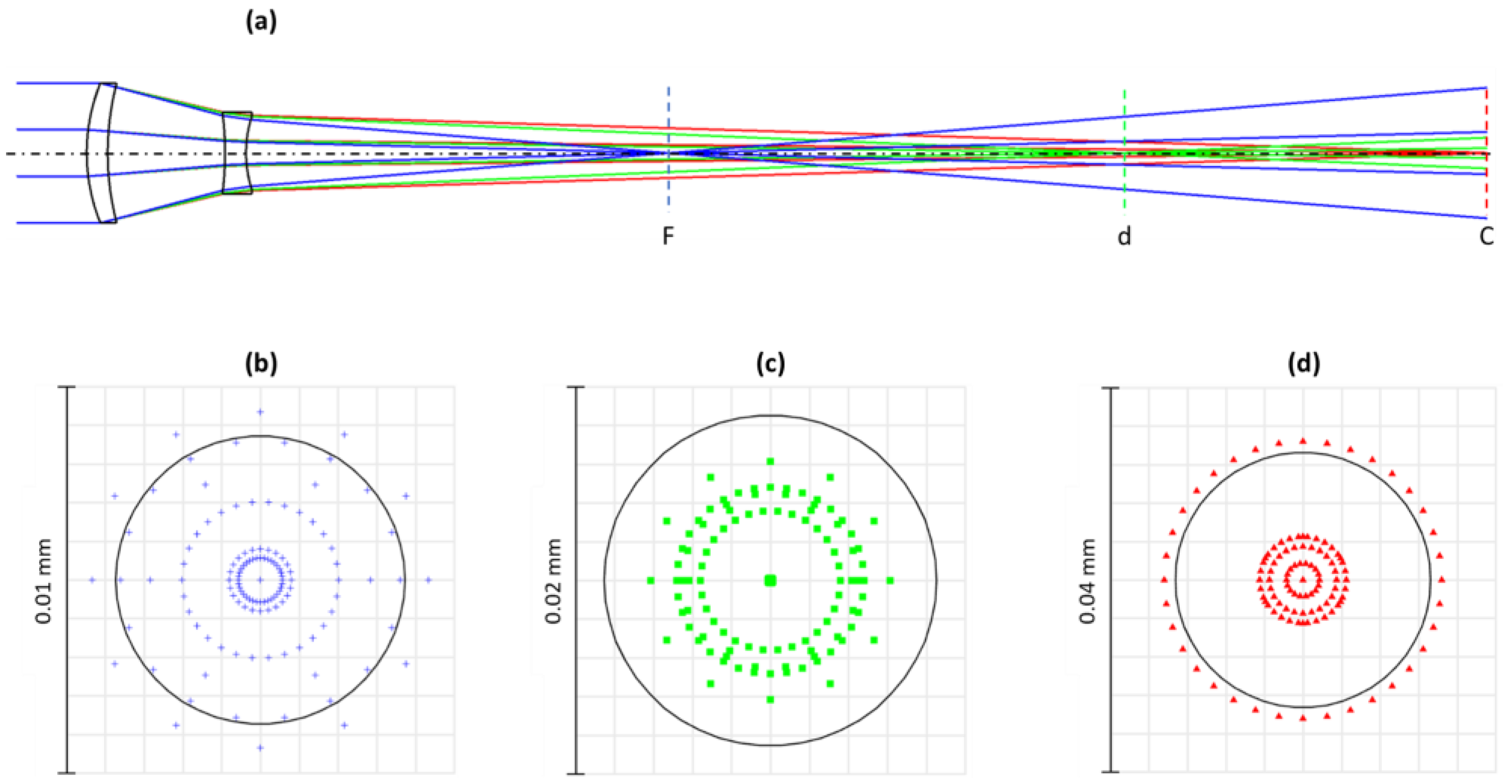
Table 3 are obtained. As an example,
Figure 7 shows the optical model and ray trace of the optimized variant for configuration 1, as well as the spot diagrams for the reference wavelengths. The black circles in the spot diagram represent the diffraction limit.
As a minimum, the lowest equivalent Abbe number of 2.07 was determined for configuration 1, which is four times lower than the Abbe number of highly dispersive ZnSe and still 40% lower than the Abbe number of a diffractive element. In configurations 3 and 4, the first element is a negative lens that converts the incoming parallel beam into a divergent outgoing cone. Therefore, the second lens must overcompensate for the negative optical power of the first lens, which is associated with small radii of curvature and significant spherical aberration. In addition, the diameter of the second lens must be larger than that of the first lens. For these reasons, configurations 3 and 4 are not preferred solutions. In conclusion, the best choice for a purely refractive system is a positive lens with a low Abbe number for the first element and a negative lens with a very high Abbe number for the second element as in configurations 1 and 2. By choosing this approach, it is even possible to obtain an extreme hyperchromatic system with an equivalent Abbe number of 4.3 using conventional materials, as shown in configuration 2.
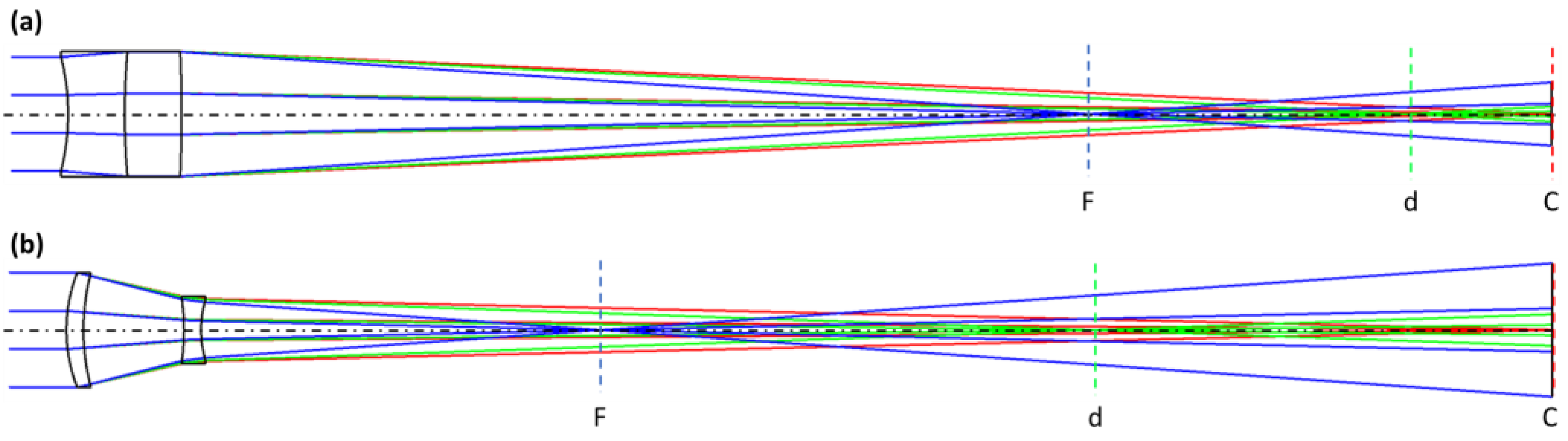
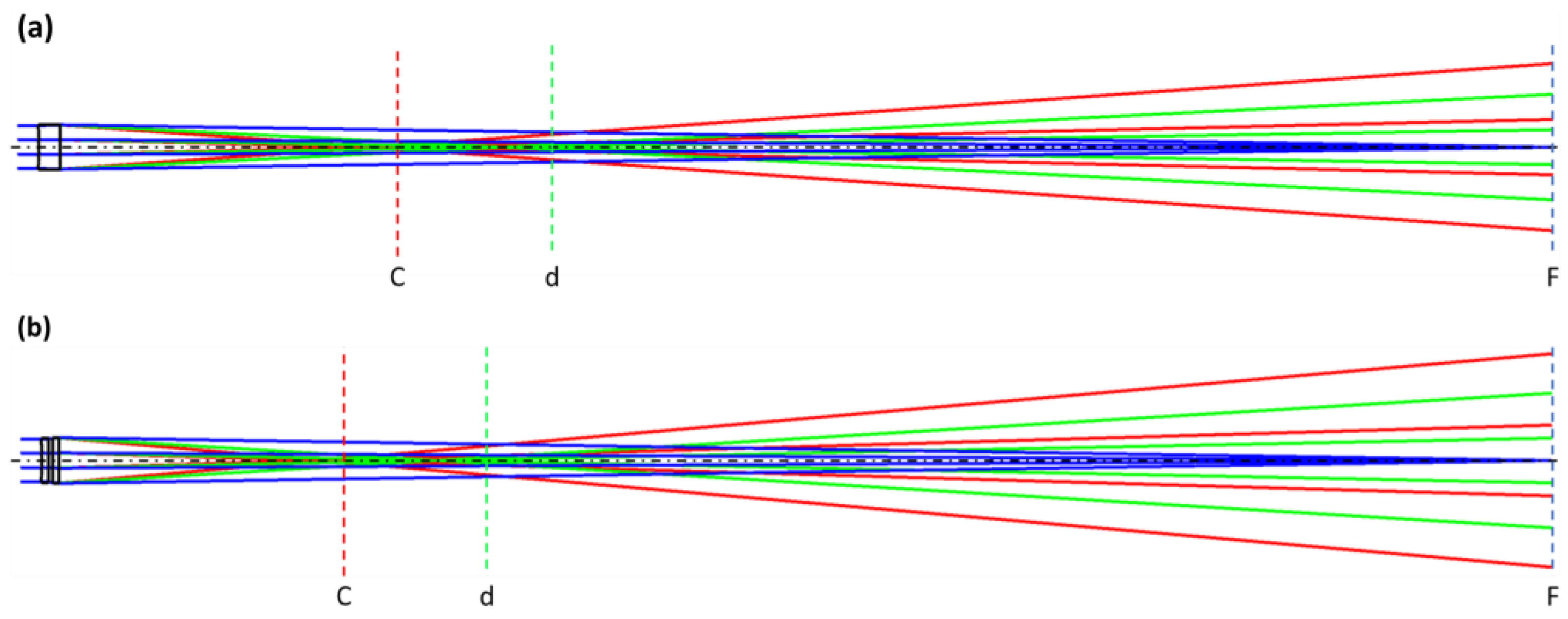
To demonstrate the advantages of the presented strategy, in particular the ability to separate the two lenses, a comparison was made with a previous approach where both lenses were in direct contact. Specifically, the pure refractive system with the lowest equivalent Abbe number was selected from [
11], which combines a ZnSe and a CaF2 lens in direct contact. With the same boundary and geometric conditions for both cases, in particular a total system length of 130 mm with equivalent Abbe numbers of 2.5 and 1.79 were obtained. This represents a 33% reduction for the new strategy compared to the previous reference approach. The most important parameters for the previous reference system and the optimized systems, including the lens distance, are listed in
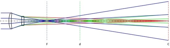
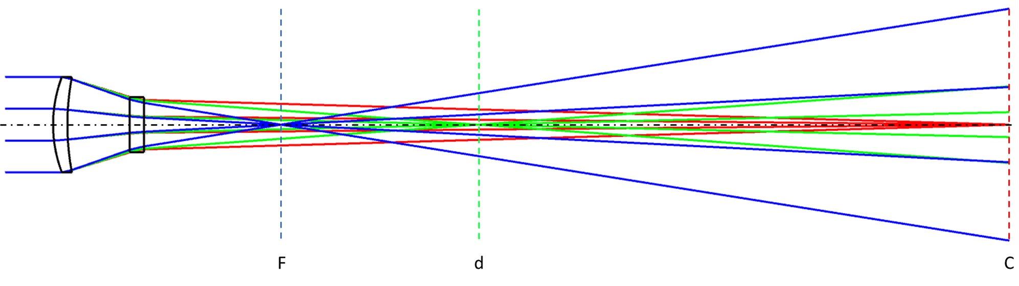
Table 4. The difference between the equivalent Abbe numbers of 2.5 and 1.79 becomes particularly clear when comparing the spectral decomposition shown in
Figure 8 (
Figure 8a reference system,
Figure 8b optimized approach). Although the equivalent Abbe number is only 40% smaller in the optimized case compared to the reference setup, the length of the spectral spread is almost twice as large. Note that in both cases the focal point for the long wavelength
has the same distance from the respective lens one, but the focal lengths for the short
and medium wavelength
are different.
6. Numerical Finding of Global Minima and Optimization for Diffractive and Hybrid Systems
For the design of purely diffractive and hybrid systems, the same sequence of numerical calculations, in particular the same boundary conditions of
Table 1 and subsequent optical design optimization was chosen. In order to numerically calculate the parameters for the systems with the lowest possible equivalent Abbe numbers, it was necessary to estimate the minimum focal length of the diffractive elements. The focal length of a diffractive element
is given by the incident height of light, which is equal to half the diameter of the lens
and the resulting angle of diffraction
.
The diffraction angle of a DOE is dependent on the desired diffraction order
, the central wavelength
and the smallest producible grating period
. For our purposes, we have assumed a minimum period of 5 µm for which a blazed profile with sufficient diffraction efficiency can be guaranteed [
30].
Substituting Formula (26) into (25) gives the following equation for the minimum focal length of a DOE. The focal length will be at a minimum when the diameter of the lens
and the grating period
are as small as possible.
With this approach, the lowest equivalent Abbe numbers were also calculated numerically from the possible focal lengths and distances for the hybrid and purely diffractive variants. Five different combinations were selected. The calculated results for the respective configurations are listed in
Table 5. All equivalent Abbe numbers obtained are significantly lower than the Abbe number of a single diffractive element and do not vary significantly between 1.31 and 1.51. In addition, the results of
Table 5 show that all combinations are characterized by a positive focal length of the first element and a negative optical power of the second element. As in the purely refractive case, a diffractive or hybrid solution with a first negative optical power seems unsuitable for a system with a low equivalent Abbe number. However, a direct translation of these configurations into an optical design show that these approaches are not applicable.
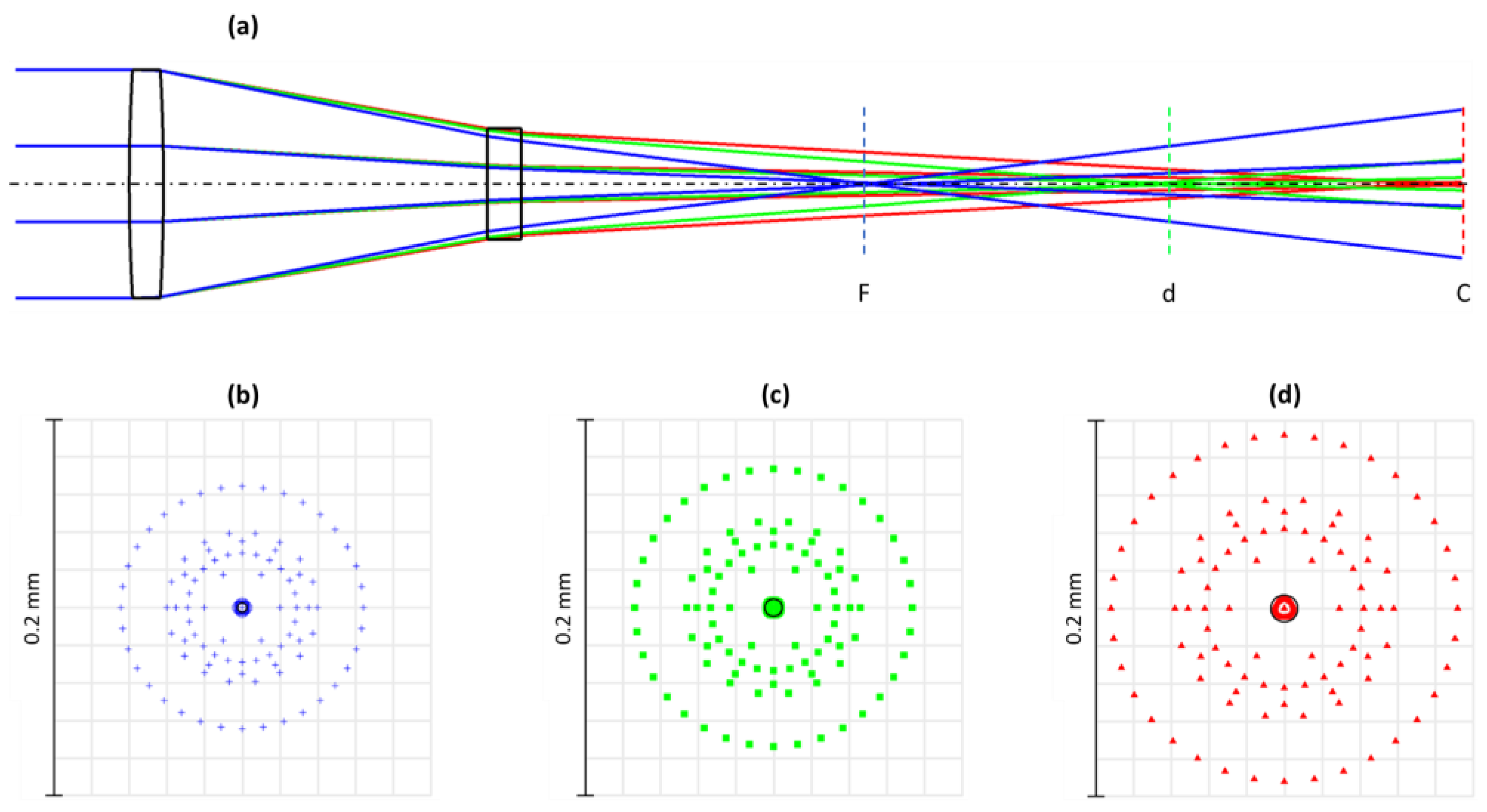
Figure 9 shows the ray trace and spot diagrams of configuration 1 from
Table 5. Obviously, the imaging quality is far from the diffraction limit (black central circle in the spot diagrams).
Although the system in
Figure 9 does not appear to be suitable for a hyperchromatic implementation, the results in
Table 5 show that diffractive and hybrid systems in principle have a high potential to achieve much lower equivalent Abbe numbers. For diffraction-limited imaging qualities, the results of the numerical calculations for the initial systems were again optimized by the optical design software. The following tuning procedure assumes similar boundary conditions and aberrations as before. For the treatment of the diffractive structure in the simulation software, the surface type “binary 2” with a normalization radius of 100 mm and a quadratic phase term (
p2 value) was specified [
28], and the beam formation was assumed with first-order diffraction. The results of the optimization process are shown in
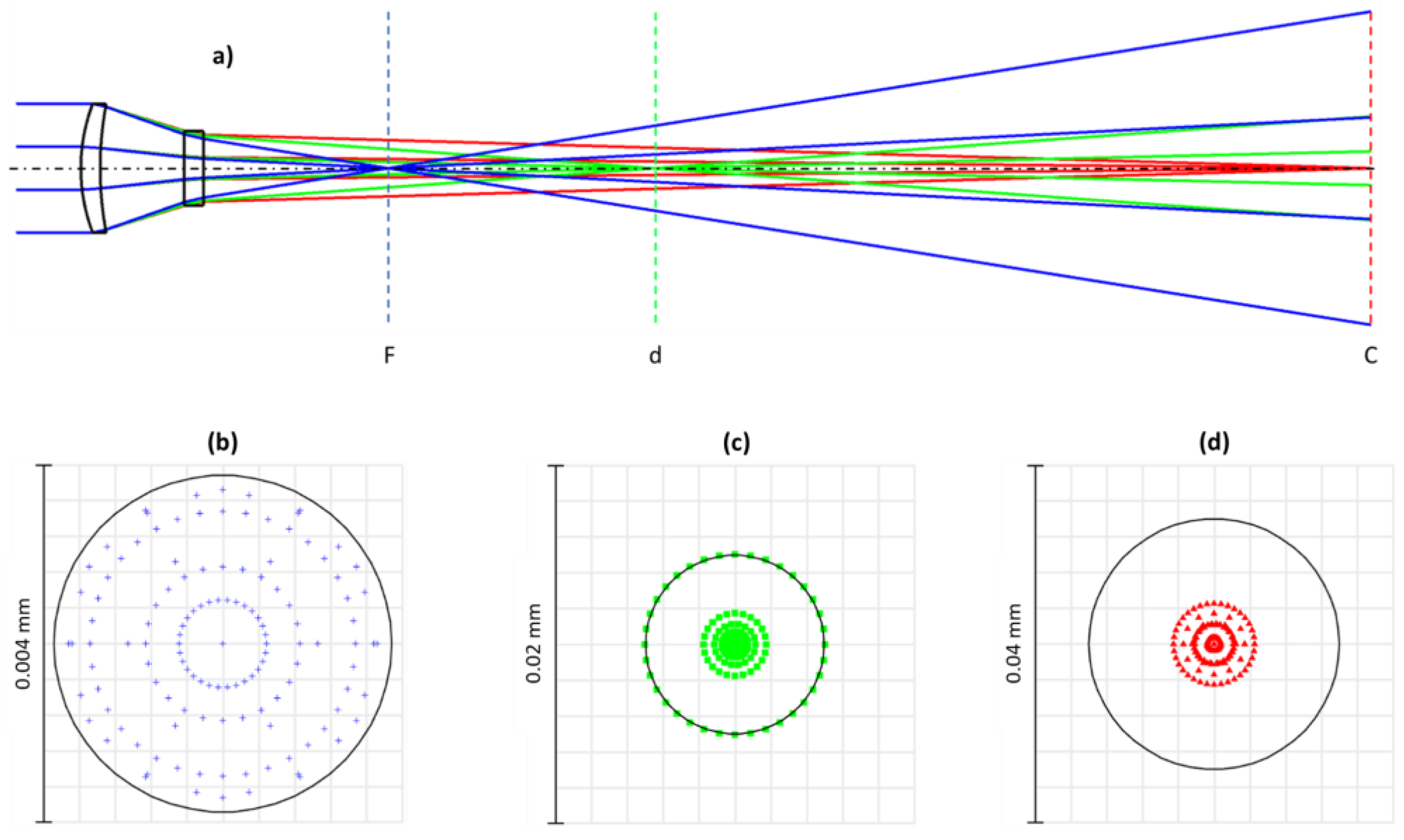
Table 6. Exemplarily, the color separation achieved for configuration 1 can be seen as a ray trace in
Figure 10a, and the high image quality of the optimized system is shown in
Figure 10b–d as the corresponding spot diagrams.
The lowest possible equivalent Abbe number (0.93) is obtained for configuration 1 with a positive ZnSe lens as the first element and a negative DOE as the second. The reverse order, first a positive DOE followed by a negative ZnSe lens, also results in a rather low equivalent Abbe number (1.04). These approaches result in an equivalent Abbe number that is approximately two times lower than the previously discussed optimized refractive systems. However, the extremely low equivalent Abbe numbers were not only achieved by using ZnSe as a material with exceptional dispersion properties. For example, for the combination of a positive DOE for the first element and a negative lens of P-SF68 for the second element; an equivalent Abbe number of 1.21 was obtained, which is about two-thirds less than the value for a single DOE (configuration 4). In summary, for a strong hybrid hyperchromatic system, a highly dispersive material (very low Abbe number) must be chosen for the refracting element, and a first positive element must be combined with a second negative element.
As before for the purely refractive system, a comparison is also made for the hybrid version with a reference system consisting of a single element combining a DOE and a refractive surface. The reference system is derived from our previous study [
11]. Compared to the optimized reference system, the design strategy presented here, which allows a distance between the two optical components, enables a reduction of the equivalent Abbe number by 27% from 0.4 to 0.29. A comparison of the parameters and ray trace of the reference and the improved systems is shown in
Table 7 and
Figure 11, respectively. By comparing the ray trace of the refractive system in
Figure 8b) and the hybrid system in
Figure 11b), it can be seen that the systems show different behavior in the distribution of the chromatic focal shifts. In
Figure 8b), the focal point of the reference wavelength d is almost in the middle of the focal points of F and C, which means that the optical system has an almost linear chromatic focal shift. In
Figure 11b), the axial distance from the focal point of the reference wavelength is much closer to C than to F, indicating that the change in image distance is not linear with the change in wavelength. Whether a linear or non-linear behavior is required always depends on the application of the hyperchromat.

 ,
, 


