Feasibility Simulation of 3D Benchtop Multi-Pinhole X-ray Fluorescence Computed Tomography with Two Novel Geometries


Abstract
:1. Introduction
2. Material and Methods
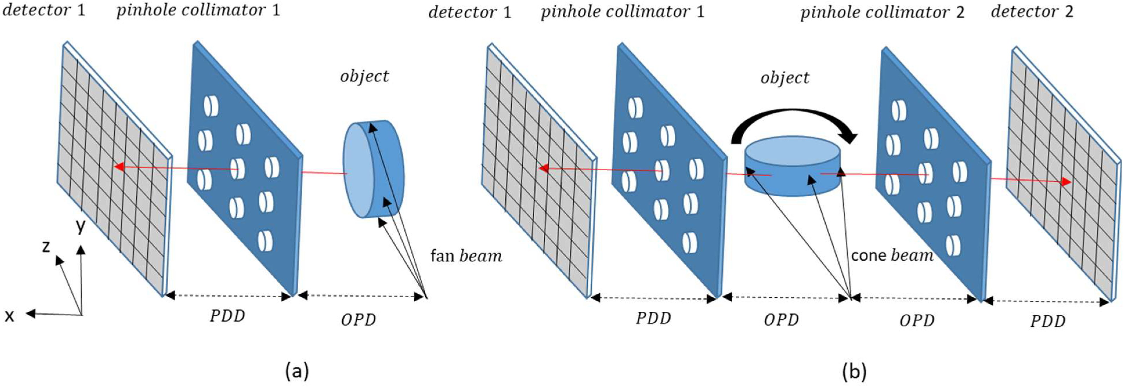
2.1. MC Model
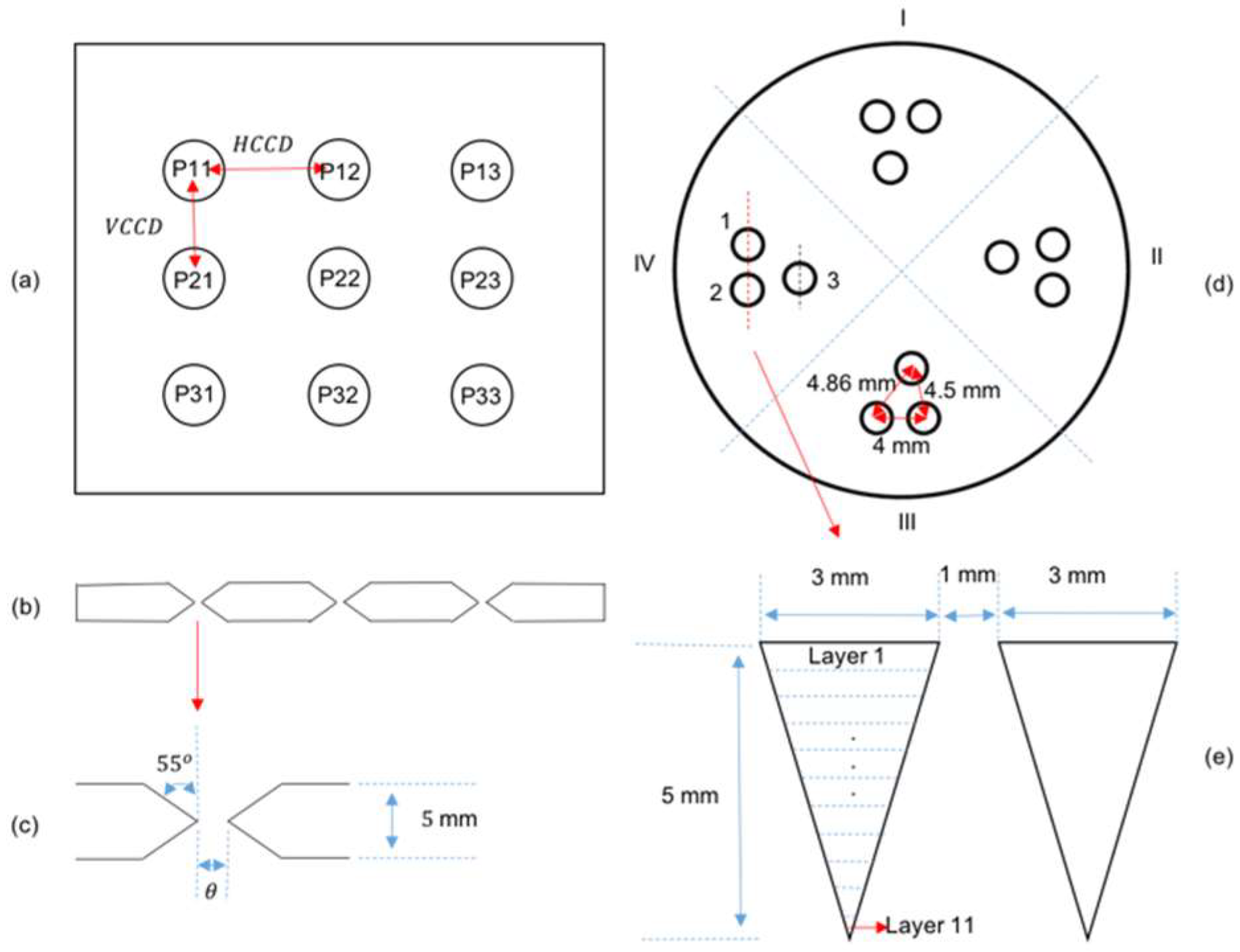
2.2. Phantom
2.3. Data Acquisition and Processing
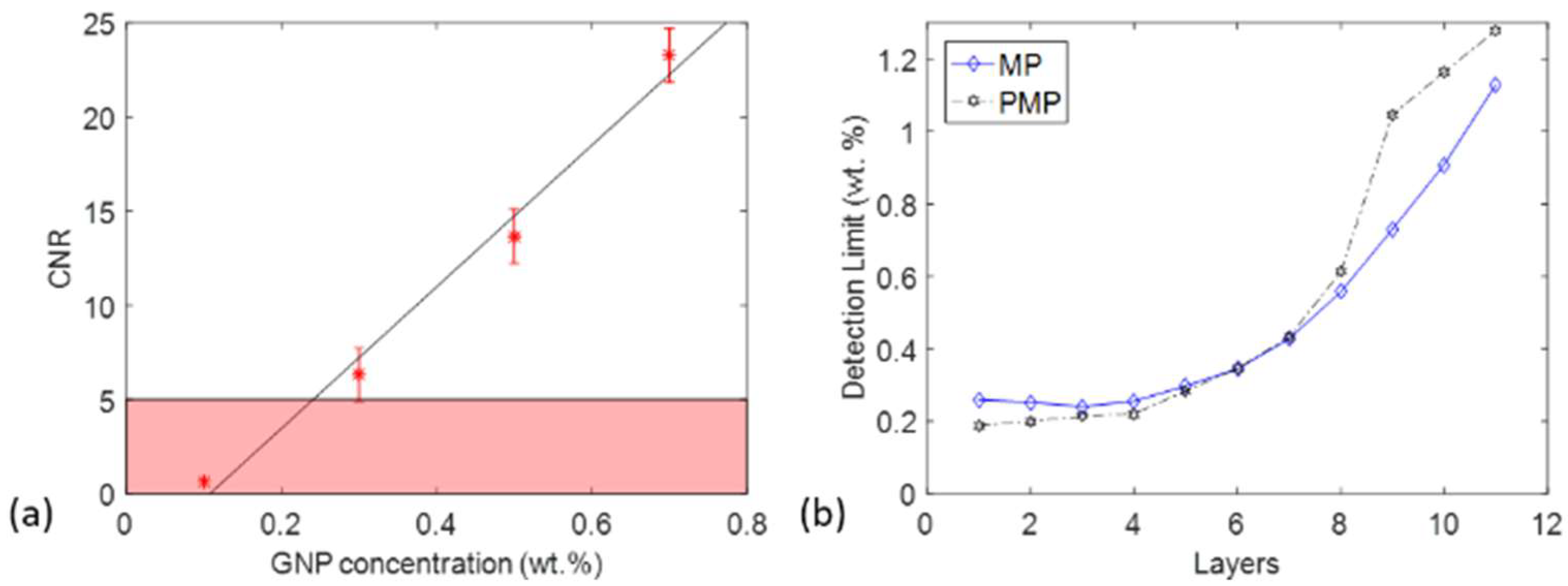
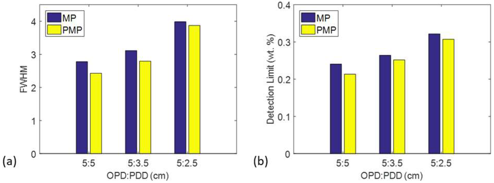
2.4. Image Analysis
3. Result
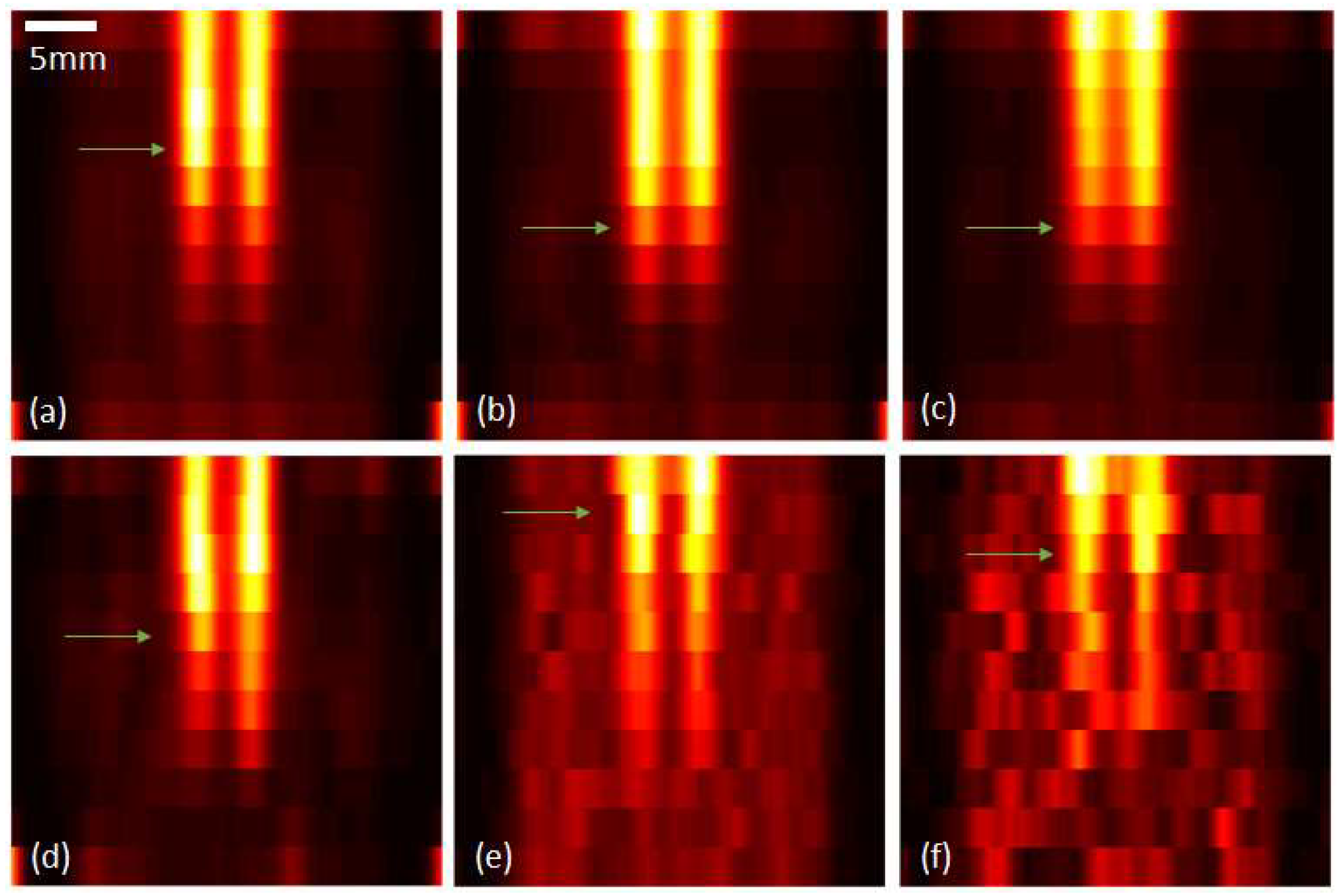
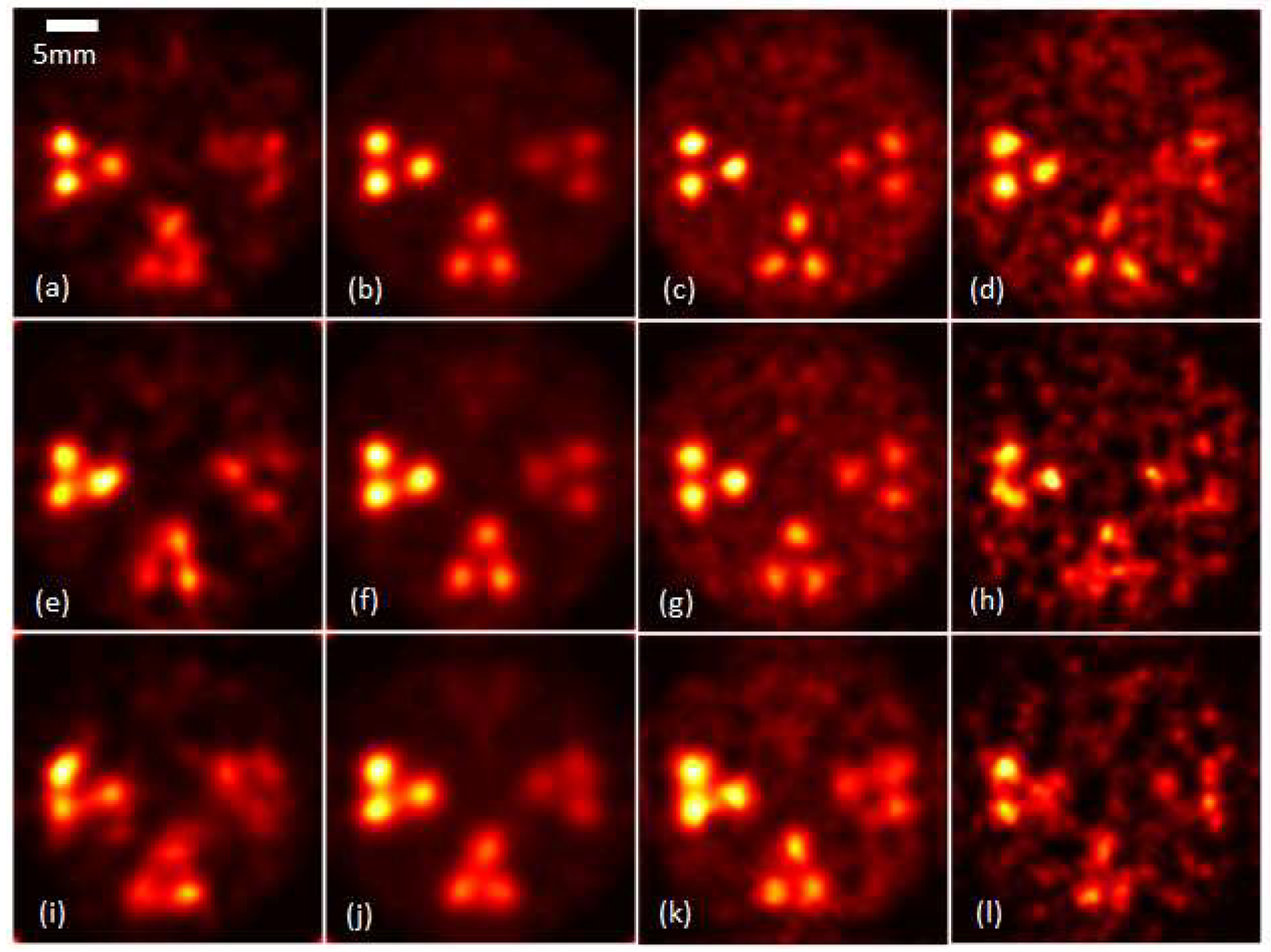
3.1. Comparison of Multi-Pinholes in Different Layers
3.2. Comparison of Multi-Pinholes for Different Magnification
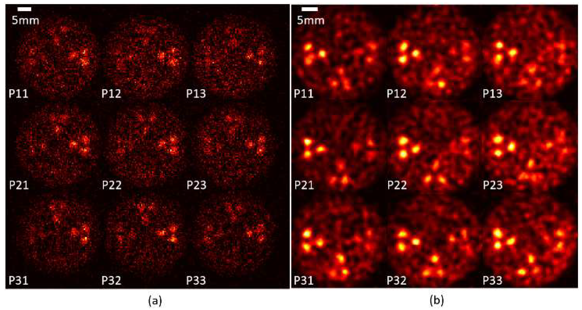
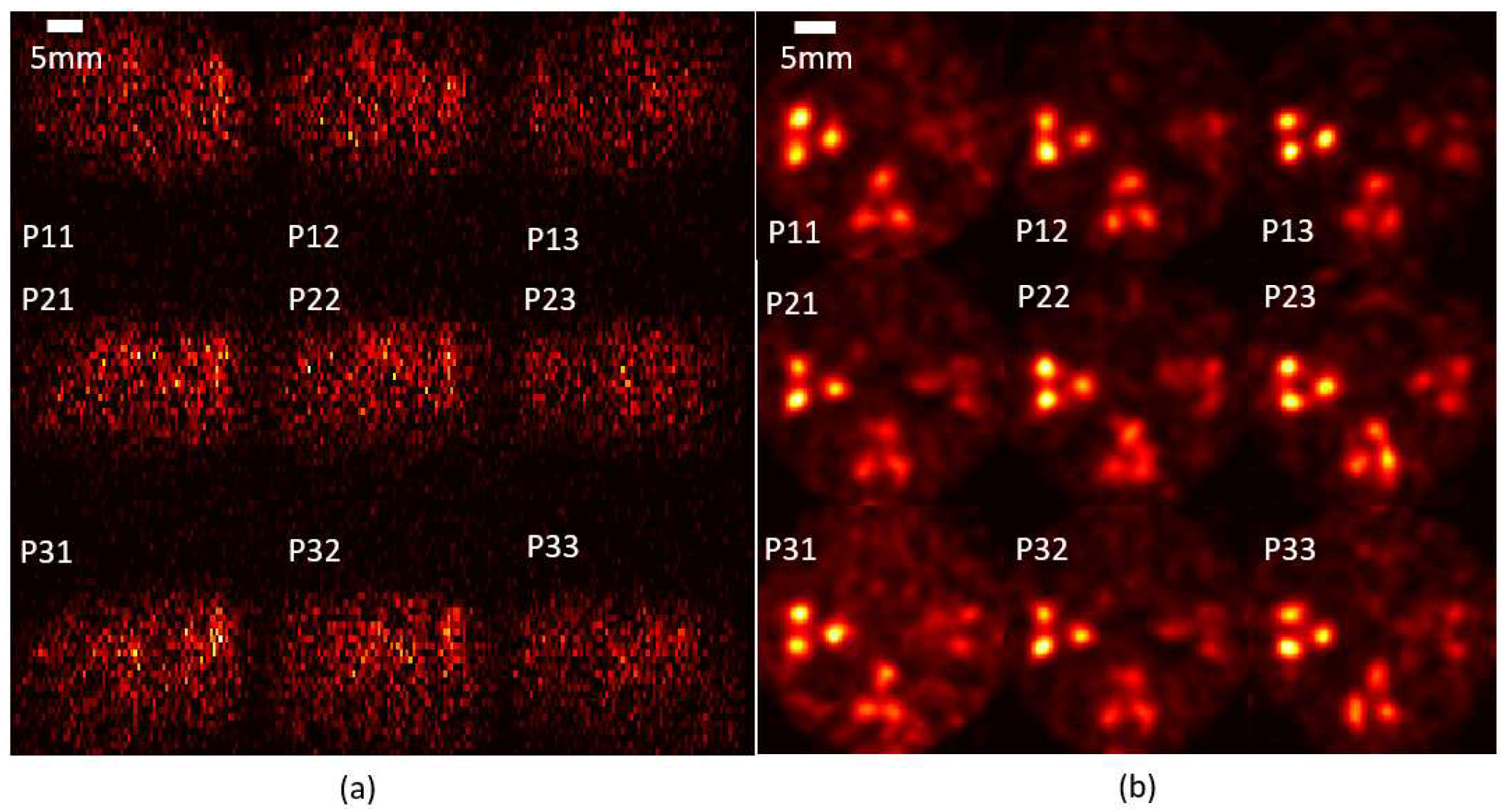
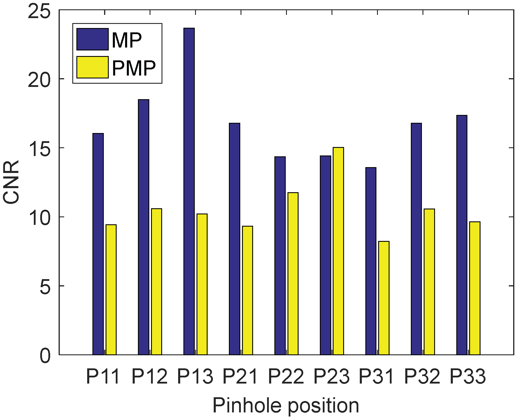
3.3. Comparison of Single Pinholes and Multi-Pinhole
4. Discussion
5. Conclusions
Author Contributions
Funding
Institutional Review Board Statement
Informed Consent Statement
Data Availability Statement
Conflicts of Interest
References
- Cesareo, R.; Viezzoli, G. Trace element analysis in biological samples by using XRF spectrometry with secondary radiation. Phys. Med. Biol. 1983, 28, 1209–1218. [Google Scholar] [CrossRef]
- Pushie, M.J.; Pickering, I.J.; Korbas, M.; Hackett, M.J.; George, G.N. Elemental and chemically specific X-ray fluorescence imaging of biological systems. Chem. Rev. 2014, 114, 8499–8541. [Google Scholar] [CrossRef] [Green Version]
- Boisseau, P.; Grodzins, L. Fluorescence tomography using synchrotron radiation at the NSLS. Hyperfine Int. 1987, 33, 283–292. [Google Scholar] [CrossRef]
- Rust, G.F.; Weigelt, J. X-ray fluorescent computer tomography with synchrotron radiation. IEEE Trans. Nucl. Sci. 1998, 45, 75–88. [Google Scholar] [CrossRef]
- Feng, P.; Cong, W.; Wei, B.; Wang, G. Analytic comparison between X-ray fluorescence CT and K-Edge CT. IEEE Trans. Bio-Med. Eng. 2014, 61, 975–985. [Google Scholar] [CrossRef] [Green Version]
- Cesareo, R.; Mascarenhas, S. A new tomographic device based on the detection of fluorescent X-rays. Nucl. Instrum. Methods A 1989, 277, 669–672. [Google Scholar] [CrossRef]
- Cheong, S.K.; Jones, B.L.; Siddiqi, A.K.; Liu, F.; Manohar, N.; Cho, S.H. X-ray fluorescence computed tomography (XFCT) imaging of gold nanoparticle-loaded objects using 110 kVp X-rays. Phys. Med. Biol. 2010, 55, 647–662. [Google Scholar] [CrossRef]
- Jones, B.L.; Cho, S.H. The feasibility of polychromatic cone-beam X-ray fluorescence computed tomography (XFCT) imaging of gold nanoparti-cle-loaded objects: A Monte Carlo study. Phys. Med. Biol. 2011, 56, 3719–3730. [Google Scholar] [CrossRef]
- Jone, B.L.; Manohar, N.; Reynoso, F.; Karellas, A.; Cho, S.H. Experimental demonstration of benchtop X-ray fluorescence computed tomography (XFCT) of gold nanoparticle-loaded objects using lead-and tin-filtered polychromatic cone-beams. Phys. Med. Biol. 2012, 57, N457–N467. [Google Scholar] [CrossRef]
- Manohar, N.; Reynoso, F.J.; Diagaradjane, P.; Krishnan, S.; Cho, S.H. Quantitative imaging of gold nanoparticle distribution in a tumor-bearing mouse using benchtop X-ray fluorescence com-puted tomography. Sci. Rep. 2016, 6, 22079. [Google Scholar] [CrossRef] [Green Version]
- Kuang, Y.; Pratx, G.; Bazalova, M.; Meng, B.; Qian, J.; Xing, L. First demonstration of multiplexed X-ray fluorescence computed tomography (XFCT) imaging. IEEE Trans. Med. Imaging 2013, 32, 262–267. [Google Scholar] [CrossRef] [PubMed]
- Deng, L.; Wei, B.; He, P.; Zhang, Y.; Feng, P. A geant4-based Monte carlo study of a benchtop multi-pinhole X-ray fluorescence computed tomography imaging. Int. J. Nanomed. 2018, 13, 7207–7216. [Google Scholar] [CrossRef] [PubMed] [Green Version]
- Luo, Y.; Feng, P.; Zhao, R.; Zhang, Y.; An, K.; He, P.; Yan, S.; Zhao, X. Simulation Research of Potential Contrast Agents for X-ray Fluorescence CT with Photon Counting Detector. Front. Phys. 2021, 9, 686988. [Google Scholar]
- Jung, S.; Sung, W.; Ye, S.J. Pinhole X-ray fluorescence imaging of gadolinium and gold nanoparticles using polychromatic X-rays: A Monte Carlo study. Int. J. Nanomed. 2017, 12, 5805–8517. [Google Scholar] [CrossRef] [Green Version]
- Sasaya, T.; Sunaguchi, N.; Hyodo, K.; Zeniya, T.; Takeda, T.; Yuasa, T. Dual-energy fluorescent X-ray computed tomography system with a pinhole design: Use of K-Edge discontinuity for scatter correction. Sci. Rep. 2017, 7, 44143. [Google Scholar] [CrossRef] [Green Version]
- Sasaya, T.; Sunaguchi, N.; Hyodo, K.; Zeniya, T.; Yuasa, T. Multi-pinhole fluorescent X-ray computed tomography for molecular imaging. Sci. Rep. 2017, 7, 5742. [Google Scholar] [CrossRef] [Green Version]
- Zhang, S.; Li, L.; Li, R.; Chen, Z. Full-field fan-beam X-ray fluorescence computed tomography system design with linear-array detectors and pinhole colli-mation: A rapid Monte Carlo study. Opt. Eng. 2017, 56, 113107. [Google Scholar] [CrossRef]
- Fu, G.; Meng, L.G.; Eng, P.; Newville, M.; Vargas, P.; Riviere, P.L. Experimental demonstration of novel imaging geometries for X-ray fluorescence computed tomography. Med. Phys. 2013, 40, 061903. [Google Scholar] [CrossRef] [Green Version]
- Meng, L.J.; Li, N.; La Riviere, P.J. X-ray fluorescence emission tomography (XFET) with novel imaging geometries—A Monte Carlo study. IEEE Trans. Nucl. Sci. 2011, 58, 3359–3369. [Google Scholar] [CrossRef] [Green Version]
- Schlueter, F.J.; Wang, G.; Hsieh, P.S.; Brink, J.A.; Balfe, D.M.; Vannier, M.W. Longitudinal image deblurring in spiral CT. Radiology 1994, 193, 413–418. [Google Scholar] [CrossRef]
- Rose, A. Vision: Human and electronic. In Applied Solid State Physics; Plenum Press: New York, NY, USA, 1970; pp. 79–160. [Google Scholar]
- Dickerscheid, D.; Lavalaye, J.; Romijn, L.; Habraken, J. Contrast-noise-ratio (CNR) analysis and optimisation of breast-specific gamma imaging (BSGI) acquisition protocols. EJNMMI Res. 2013, 3, 21–33. [Google Scholar]
- Miceli, A.; Thierry, R.; Bettuzzi, M.; Flisch, A.; Hofmann, J.; Sennhauser, U.; Casali, F. Comparison of simulated and measured spectra of an industrial 450 kV X-ray tube. Nucl. Instrum. Methods A 2007, 580, 123–126. [Google Scholar] [CrossRef]
- Redus, R.H.; Pantazis, J.A.; Pantazis, T.J.; Huber, A.C.; Cross, B.J. Characterization of CdTe detectors for quantitative X-ray spectroscopy. IEEE Trans. Nucl. Sci. 2009, 56, 2524–2532. [Google Scholar] [CrossRef]
- Lange, K.; Carson, R. EM reconstruction algorithms for emission and transmission tomography. J. Comput. Assist. Tomogr. 1984, 8, 306–316. [Google Scholar]
- Shepp, L.A.; Vardi, Y. Maximum likelihood reconstruction for emission tomography. IEEE Trans. Med. Imaging 1982, 1, 113–122. [Google Scholar] [CrossRef]
- Guo, J.; Feng, P.; Deng, L.; Luo, Y.; He, P.; Wei, B. Optimization of Detection Angle for Pinhole X-Ray Fluorescence Computed Tomography. Acta Opt. Sin. 2020, 40, 0111017. [Google Scholar]
- Nowotny, R. XMuDat: Photon Attenuation Data on PC; IAEANDS-195; Nuclear Data Services: Vienna, Austria, 1998; Available online: http://www-nds.iaea.org/publications/iaea-nds/iaea-nds-0195.htm (accessed on 1 August 1998).
- Ahmed, M.F.; Yasar, S.; Cho, S. A Monte Carlo Model of a Benchtop X-ray Fluorescence Computed Tomography System and Its Application to Validate a Deconvolution-Based X-ray Fluorescence Signal Extraction Method. IEEE Trans. Med. Imaging 2018, 37, 2483–2492. [Google Scholar] [CrossRef]


| MP | PMP | |||||
|---|---|---|---|---|---|---|
| OPD:PDD | 5:5 | 5:3.5 | 5:2.5 | 5:5 | 5:3.5 | 5:2.5 |
| 9PH | 0.24 | 0.26 | 0.32 | 0.21 | 0.25 | 0.31 |
| 1PH | 0.32 | 0.32 | 0.42 | 0.35 | 0.47 | 0.41 |
Disclaimer/Publisher’s Note: The statements, opinions and data contained in all publications are solely those of the individual author(s) and contributor(s) and not of MDPI and/or the editor(s). MDPI and/or the editor(s) disclaim responsibility for any injury to people or property resulting from any ideas, methods, instructions or products referred to in the content. |
© 2023 by the authors. Licensee MDPI, Basel, Switzerland. This article is an open access article distributed under the terms and conditions of the Creative Commons Attribution (CC BY) license (https://creativecommons.org/licenses/by/4.0/).
Share and Cite
Ye, B.; Deng, L.; Jiang, S.; Cao, S.; Zhao, R.; Feng, P. Feasibility Simulation of 3D Benchtop Multi-Pinhole X-ray Fluorescence Computed Tomography with Two Novel Geometries. Photonics 2023, 10, 399. https://doi.org/10.3390/photonics10040399
Ye B, Deng L, Jiang S, Cao S, Zhao R, Feng P. Feasibility Simulation of 3D Benchtop Multi-Pinhole X-ray Fluorescence Computed Tomography with Two Novel Geometries. Photonics. 2023; 10(4):399. https://doi.org/10.3390/photonics10040399
Chicago/Turabian StyleYe, Binqiang, Luzhen Deng, Shanghai Jiang, Sijun Cao, Ruge Zhao, and Peng Feng. 2023. "Feasibility Simulation of 3D Benchtop Multi-Pinhole X-ray Fluorescence Computed Tomography with Two Novel Geometries" Photonics 10, no. 4: 399. https://doi.org/10.3390/photonics10040399